COMPUTER SIMULATION OF DIRECTIONAL SELECTION IN LARGE POPULATIONS. II. THE ADDITIVE x ADDITIVE AND MIXED MODELS

COMPUTER SIMULATION OF

DIRECTIONAL SELECTION

IN LARGE

POPULKmONS.

11.

THE

ADDITIVE

x

ADDITIVE AND

MIXED

MODELS

S. S. Y. YOUNG

C.S.I.R.O., Division of Animal Genetics, P.O. Box 90, Epping, New South Wales, Australia

Received November 29, 1966

HE

change of the additive genetic variance ( a n 2 ) under selection and the ability of the estimate of heritability in the narrow sense

(LUSH

1940)

(h’)

to predict genetic gain are important considerations in formulating breeding plans and understanding selection experiments. YOUNG ( 1966) has discussed the value of prediction and the decay of additive genetic variance when the character is controlled by additive genes (the “A model”) and genes with some dominance (the “D model”).

He

assumed control by ten loci, and simulated selective breed- ing by computer.

In the same series of investigations further models were used, the results of which are reported here. One was epistatic (the “E”), in which the genetic value of each pair of loci was assumed to be determined by the product of their respective additive values

(A

x

A interaction),

In

the A,

D

and

E models the ten loci of

each individual were assumed to show a uniform gene action, either all additive, all dominance, or all epistatic.

In

addition to these, four slightly more complex genetic situations were investigated,

in.

each of which, a fraction of the ten loci was assumed to show one effect (e.g. additive or dominance) and the remaining fraction a different effect (e.g. epistatic). These will be referred to as mixed models, and a detailed description of each will be given later.

FRASER (1960) was the first to use an epistatic model in computer simulation of selection though his results do not bear on the problem studied here.

GRIFFING (1960) reported the theoretical consequence of directional selection with a character controlled by genes showing A

x

A epistasis.

A most interesting finding was that decline of the population mean was an expected consequence of

relaxation of selection, without recourse to natural selection. GRIFFING also presented an approximation for predicting selection gains in a large population, with A X A epistasis. GILL (1965a) simulated genetic advance under truncation

selection for some small populations (8 to 32 individuals). The trait under selec- tion was assumed to be determined by 40 loci and four genetic models were used. He found that under an A X

A conditional epistatic model predictions of gains

from GRIFFING’S formula were in most cases overestimates, and concluded that random genetic drift plus changes in genetic variance had been responsible for the disagreement.

In a different report, GILL (1965b) again simulated gains by selection in small

74

S . S . Y. YOUNG

populations (8 to 32 individuals), with nine other genetic models. The rates of advance differed widely, depending on the model assumed. In general, larger populations attained higher means at the end of 30 generations of selection, indi- cating that the smaller the population the greater the loss of favourable alleles, while genetic advance was faster with the conditional A

x

A than with the addi- tive model.

The A X A model used here differs from GILL’S, while the mixed models have not previously been analysed. Again, as in the first paper of the series, the predic- tive ability of heritability ( h 2 ) and changes under selection in the additive genetic variance ( ua2) were the main problems under consideration.

The

parameters and the computer programme: The parameters used in the present work were the same as in the previous paper. Briefly these were: (1) The size of the unselected population in each generation was 1000; (2) The character under selection was assumed to be controlled by ten loci with two alleles at each locus; ( 3 ) The initial gene frequency for each allele was set at 0.5;

(4)

Three selection intensities (I) were used. These intensities

(I

= lo%, 50% and 80%)

refer to the proportions of individuals saved for breeding; (5) The character under selection was modified by a normally distributed random factor and three levels of initial heritability (h2 = 0.1, 0.4 and 0.9) were assumed; (6) Three recom- bination probabilities ( r = 0.05, 0.2 and 0.5) between adjacent loci were used and these were assumed to be constant throughout 30 generations of selection.

The computer programme used was essentially the same as before. The opera- tions again mimicked a population under random mating with truncation selec- tion. Each population started with a fixed combination of I , r, h’ and was selected for 30 generations under each genetic model. There was a slight technical differ- ence in the programme when the epistatic model was used; genetic values corre- sponding to gene doses of each pair of loci were read into genetic value storages. Apart from this, the programme remained unchanged. Additive genetic variances were again calculated by the regression method and the nonadditive variances were obtained by differences. Further details of the computer programme and the parameters used have been described in the first paper of this series

(YOUNG

1966).

The Additive x Additive ( E ) Model

The genetic value of a pair of loci was assumed to be the product of their respec- tive values. I n particular, assuming the additive values of A A , Aa and aa to be 2 d / 2 , d / B a n d 0, then for two adjacent loci the genetic values for the different genotypes were:

A A Aa M

BB 8 4 0

Bb 4 2 0

bb 0 0 0

SIMULATED SELECTION 75

loci. Thus loci 1 and 2, 3 and 4, were assumed to form two units, and no inter- action was assumed for loci 1 and 3 or

2

and 4. The programme therefore simu- lated only a fraction of all possible 2-factor A X

A

interactions. This may be partly compensated by the higher scale (e.g., AABB = 8, AaBB = 4, etc.) used, compared with A(2, 1, 0 ) and D(2,2, 0). The genetic value of an individual was calculated by summing the genetic values of the five pairs of interacting loci.

Replicated runs. Examination of the results of the repeated runs under identical parameters, but different random sequences, showed that the agreement between runs for E were as good as those for A and D. Under high selection pressure (high heritability and selection intensity) the agreements were excellent, while under

low selection pressure the runs agreed not quite as well. Tightness of linkage did not appear to effect the results. I n Figure 1A and B two extreme cases are shown as illustration. I t may be concluded that the effect of genetic drift was unimportant in this analysis.

(A) I = SO%, r = 0.5. (B) I = IO%, r = 0.5.

Predictive value of h2. The present results showed that the prediction of long term genetic advance, assuming constant heritability, again proved to be of limited

c

10 20

5 10 15 2 0 25

GENERATION

5 10 15 2 0 25

GENERATION

FIGURE 1.-Additive x additive model: Replicate runs of six populations with the same recombination probability ( r ) and different initial heritahility ( h z ) under different intensities of

76 S . S. Y. YOUNG

40.

2 0 .

IO.

T-

I m IS 20 25

GEMRATION GEMRATION

FIGURE 2.-Additive

x

additive model: Comparisons between realised and expected genetic advance with I = IO%, r = 0.6, and t w o levels of h2 (0.9 and O.l), h? being assumed constant throughout.

value. Figure 2 illustrates this for two extreme situations when hz = 0.9 and

h2

= 0.1. Under high selection pressure the constant h2 predicts gains reasonably well for 3 or 4 generations, but under low pressure the predictions were inaccurate after 1 or 2 generations.

Predictions of advance based on

h2

values calculated in each generation were also made, comparisons between predicted and realised gains being shown in Figures 3A,

B,

C and

D.

When selection intensity was high (I = 0. I O ) , agreement was good for the 4 to

5

initial generations of selection for all levels of hz and r, but thereafter predictions tended to give underestimates (detailed data not

shown). In later generations predicted gains reached a plateau at values below the realised figures. Similar results were obtained when Z = 50% (Figures 3A, B)

.

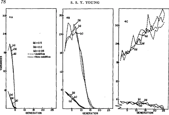
The agreement in this case was again fairly close, and a lower hz did not lead to greater discrepancy. Again, however, the predictions tended to give under- estimates. When selection intensity was low (Figures 3C, D) agreement was only good when hz was high or intermediate. When hz and selection intensity were both low, agreement was poor, and in these circumstances predictions were in excess of the actual gains over 30 generations of selection. Under moderate or high selection pressure the populations all reached the maximum expected value, indi- cating that there was no loss of favourable alleles during selection.

Changes in additive genetic variances. A characteristic of the present results was the increase in o A z for several generations of selection in all populations. (Figures 4A, B, C ) . The reason for this has been investigated and will be dis- cussed in a later section of this paper. Under high selection pressure (Figure 4A) uA2 showed a small increase f o r two generations, followed by a rapid decrease; the

77 SIMULATED SELECTION

0

m

I

a

78

r---

Wr=O05

-

=Non-additive ----AddifiW

5 IO 15 20 25

OMERATION

S. S. Y. YOUNG

I

I-.b.,

5 IO I5 20 25

GENERATION

FIGURE 4.-Additive

x

additive model: Changes in the additive and nonadditive genetic variances under different selection intensities (I) for populations with different initial heritabilities

(h2) and recombination probabilities ( r ) .

(B) I = 50%, h2 = 0.4.

(A) I = IO%, h2 = 0.9. ( C ) I = 80%, h2 = 0.1.

vanished after 4 generations. Under intermediate selection pressure (Figure 4B)

the additive genetic variance increased for 7 to 8 generations then showed a rapid decline and was gone by 17 generations; the nonadditive variance declined from the start and was gone by 12 generations. Under low selection pressure (Figure

4C) the additive genetic variance increased rapidly even up to 25 generations; the nonadditive variance showed a general slow decline, but did not entirely disappear.

An interesting feature of the changes in genetic variance was that when selec- tion pressures were mild, tight linkage tended to inhibit the increase in uA2 (Figure

4B, line C ) . This may be the result of the initial gene frequencies assumed for each pair of loci. As will be discussed later, when two interacting loci are equal

in gene frequency the additive genetic variance is at a local minimum, hence tight linkage would tend to prevent the attainment of optimal combinations of frequencies for higher uA2. The effect of linkage on changes in variance was not

apparent when selection pressure was high (Figure LEA).

Figures 4A, B and C represent only a fraction of the results, but they are typical examples and there seems little point in presenting extensive figures in great detail.

Mixed Models

SIMULATED SELECTION 79

80 S . S . Y. Y O U N G

esting to present detailed descriptions of results obtained under different sets of circumstances. In this section, therefore, results will be very briefly discussed, while a summary for all models will be given in DISCUSSION.

The A

+

D model. Five additive and five dominance loci were assumed. The genetic values assumed for A and D were given in the first paper. Agreement between expected and realised gains was close, even under low selection intensity and low heritability. Figure 5A shows a typical set of results when 1 = 0.50 and r = 0.50. The agreement obtained under the present assumption was as good as for the additive model, and there was again no evidence of any loss of favourable alleles nor of any appreciable effect of linkage on genetic progress. The curves for the decay of the additive genetic variance were of the constantly decreasing type and were again mainly influenced by both h' and 1. The nonadditive vari- ance in most cases persisted in the population for many generations. A typical set of results is shown in Figure 6A for 1 = 50% and h' = 0.4 with different linkage values.

The A

4-

E model. Four additive and three pairs of A x A loci were assumed. A most striking feature of the results was consistent under-estimation by the predicted gains when selection pressures were high or intermediate (Figure 5B), but when selection pressures were low the situation was reversed (data not shown here). Discrepancies between the predicted and the realised gains were often appreciable; under high selection pressure the mean error of the prediction amounted to something like 25% of the total advance, while under low selection pressure the mean errors were about

5

%

of the range. Disagreement was evident even in the early generations of selection, particularly when selection pressure was high or intermediate. The cumulative effect of the lower predicted gains resulted in large differences in the realised and predicted plateaus after the ex- haustion of genetic variances.

Changes in the additive and nonadditive variances (Figure 6B) were again functions of h' and I , and both variances showed the characteristic rise for a few generations, with subsequent decline. The reason for this will be discussed later. The D

+

E model. Four dominance loci and three pairs of A x A loci were assumed. The results are similar to those for the A

+

E model. Figures 5C and 6C are typical results. Under high selection pressure the mean error of prediction for each population was even higher than that for the A

4-

E model (see Table 1 )

,

but under low pressure the predictions were more accurate. The pictures of decay in genetic variance were again similar to those for the A

+

E model, except that the nonadditive variance survived much longer. The similarity of the results between the A

+

E and D

+

E models was no doubt due to the inclusion of the

A x A loci, as the scales used for these were higher than those for the A and D

models.

The A

+

D

+

E model. Three additive, three dominance and two pairs of A x A

SIMULATED SELECTION

18- 6 B 18. 6A

‘1

I

I --

15 20 2s 5 IO I(I

81

GENERATION GENERATION

FIGURE 6.-Mixed models: Changes in the additive and nonadditive genetic variances with

I = 50%, hz = 0.4.

(A) A+D model. (B) A+E model. (C) D+E model. (D) A+D+E model.

extremely high selection pressure, but under low pressure both variances showed first a slight increase and then a very gradual reduction of uA2 but a gradual

increase in the nonadditive variance.

Comparison Between Models

3

0 2 E 9 '2

2U .d 5

.E1

z

5

%

g &

3

.B

2

3

3

5

g

B

5

j

- B

,x

3

.;

;

,%

.$

53

. s e

.-

F p

2

!

.2

i j M

E 1 w w

c

3

;

.$

$

s

Y .- $

I

PY .n E

$

c

E \ a l O E M m w m " q ~ k ? + & q

~~~~~:~

% ? ? % $ ? %

m ~ $ 5 - m m m m o l h m - " - m m * + o l m

- r y 7

4

r 5 y y q - q

2

ZE:'".

L!

sG a m + * m o m c - l m o l m m o m m d - m c - l h m - y W m . q m q 9 - a h m ~ q m q k % + + - e w I 56

0 - 7 ~ 7 0 ~

o o c j y ~ ' ~ o 7

00- NON 1 I l l I

I l l

7

+ \ a h o a m m

~ e

g!:

b - , m y m % 8

a $ : $ g q e

e s w s 3 $ w

~ d ~ 2 g - mo m o a m o m e-" m z - j - ~ ~ m ~

I l l

7

1 1 1 ' 7

8

2

$ E X

11

!!

C . c 1 o e m h - m

CI $ 5 q k " o ' 4 y w & F a q i ? s ?

$ g s q ? q $

I I I l P

""rill"?

I I I

-7

O o m m m 0

2>&

h a m w w a * m o h m * z m m + * m * - m

o : E 0 " i 1 9 ' 4 ' 4 " k 909h.W" . @ ! " 9 ' ? 9 L ? ? k

" 1 7 7 7

" I ' i ' i

'i

% M I l l

i

I I c .

L_

$3

o - m m m o I I l o - m m m o I l l I I l l

7

2

$ 2 -""'zQo I I $ ' ?

4

@(TT'J"i@(S;

f T q y 7

F

L

I

E@ . o o ~ 7 T o ~

N . ? @ ! " 9 - ' 1 9 9 k % ? ? k n

I

4 4 ' i " i ? ' i l

4 0 4 - i . T o - i

5

m a z g s a??"??-: ? F k ? Y ? G

p4z5%

r;l.

!!

9%

g%gzggs

% ; ? % ? g g $ O q C J m y h

+

4

Ea

' i P l T ?

o 0 4 T T ? T

40-i'io-i

+-

o ; $ f i s y q - a q q * q q w m 3 ; 2 8 3 % 8 % %

:

48

0 , " m W ~ ~ m m * 8

q q q & s . q a

'3

" T T T ' i T

0 0 0 - - 0 0 0,

m

w s :

g 2 = o c j T ' 9 f ' i m j

L!

Em& y m m , y - q ? y m ? f ? F

p ; G ? @

1

I 5 5

" o r i 7 4 1

9 9 " 4 9 4 4

f m - o S o

;

1 z a

X o T T f o ?

404"'i9''i

~ ~ a O O O a O

1

En $ % 3 g F r a s q 0 0 0 - - 0 - 3 s & g x s s F $ S ? $ ! s O 1

f 4 m - o 7 2

,~

c

En o - m a m o

2

$E$ -~co~~aO b b h m m + w m O m m h + m ui

s s $ g : $ l g ^

% 3 ? g ; s s

Z e r q a q G

o - - m m o m a

g

I l l 1 8

'2

I I

*\a

_is:

m o - m m m m H o - h - a m M o m o a m m w

@!a^???" 9 q ? " k y c ! W " . " % ? W ' 4

+

z z g z c g > m o - o m + w - w - w a h m m 4 II

g

22% o o m + . - m - m o - h

2

$ E X O W T Z 2 7 3

4yT?rT

I l l 1

'i

n

kl"

h m m h m d

E!!

I I I

a

82% m + w w m m w m o l o m m

2

$ z $

o + m m r o o m - o l c o m m m c i G - ~ ~ m 1

.g

I 1 I 3

8

B

h m c o y c o q y q ~ m m - q y h k o m k h I1

I ' i ?

7

4

l ' i 7 l - i

!!

0 . m - m m m 0, a g ~ m o

-""-i-iI

I I

a

z\a, z m m o m m m m o h o h o l m N m m m h h m

w

4 " i 7 - i 7 P

* q m m - - i m

I

-8

&ad.

- * * * * * U ? - * m h O m

d

u m E y q " m 1 k '4"*."@!'9 " " 9 o l . 9 4 9

'g

g

2

i g z

O m q S C j r ?

' i i " y T ? T

4 T m " " j 0

a

m ₁₁

_!!

_3%

3

- m * m w o o m h m m o

y , k e , , y . . - . @ ! q m 8 8

s:?z.s;F

b B II

3 2:s ? ? ? S ? $ 8 ? h . " - . c ! ' D ? " ? ? a l " = ! k .^

2 $ 2 2 = - a " - - I I I

'i

1 - I

!!

e .

I I I I

4 4 4 4 - i o - i

2>&

a m o + - w m m * ~ m - o m h ~ - m *

$>& e o m h ~ w m c - l o a h w w m m ~ h m fl

o g 7 g y 4 y

w - o m m o m

-

3

z

H

01 a e

N b n 4 n

+

0 4 ~ ~ r l w w ~ w ; c ~ i w w w n w o : c a w w w n w

II

+ + + +

+ + + +

I I

+ + + +

4 n q n N 4 n - t n N

+ 2

m

+ :

4 ;. 4 :

-i.

-

...

.- 4

.s

.3 .-

C _H

c H

i

-2

1

SIMULATED SELECTION 83

predicted gain gave an under-estimate. Also, different models have different ranges of genetic advance; f o r example, under the A model the mean increased from 10 to 20 units, while under the E model the mean started at 10 units and reached a plateau at 40 units. To facilitate comparisons between models, mean differences in each model were also expressed as percentages of the total range of advance. The variances of the difference for the first 12 generations are shown in Table 2. From Tables 1 and 2 it is evident that predictions with E were more erratic than with A or D, although under high selection pressure of means of errors of prediction for D were higher. It is interesting to note that means and variances of errors of prediction were almost always higher under mixed models involving epistasis. I n such models, although only a portion of the total number of loci were assumed to be interacting, predictions of gains were much more erratic than with pure epistasis.

Among results obtained for mixed models which assumed two types of gene effects (A

+

D, A

+

E, and D

+

E ) , predictions assuming the

D

+

E effects were in general less accurate. When some of the loci in the D

+

E model were replaced by additive loci (A

+

D

+

E

model) there was in general an increase in the size (on a percentage basis) of errors of prediction. This is unexpected as it seems

TABLE 2

Variance of differences between estimated and realised genetic advances

I=80% I=50%

r=0.50 r x 0 . 2 0 r z 0 . 0 5 r=0.50 r=0.20 r z 0 . 0 5 -

0.001 0.002 0.002 0.009 0.055 0.057 0.892 1.140 1.687 1.395

0 . 0 4 0.004

1.819 1.902

0.023 0.004 0.017 0.012 3.161 0.028 0.161 0.744 0.272 0.512 0.024 0.008 0.738 0.569

0.038 0.061 0.070 0.030 1.958 2.815 0.555 0.591

0.049 0.225 0.050 0.034 0.074 0.145

0.006 0.006 0.225 1.803 1.918 0.009 1.961 0.016 0.018 0.107 0.370 0.362 0.013 0.508 0.047 0.046 1.747 0.172 0.140 0.030 0.095

0.003 0.004 0.008 0.011 0.018 0.017 0.401 0.181 0.348 4.863 5.906 6.385 4.800 5.007 7.311 0.039 0.050 0.045 3.219 4.031 3.787

0.011 0.007 0.015 0.027 0.015 0.013 0.170 0.031 0.161 2.887 9.256 5.484 3.958 5.029 4.837

0.044 0.025 0.024 2.548 3.105 3.084

0.020 0.036 0.033 0.040 0.036 0.038 0.175 0.127 0.469 2.825 0.712 2.269 1.892 0.873 2.265

0.025 0.048 0.036

1.001 1.598 1.973

z=10%

r=0.50 r=0.20 r=0.05

0.049 0.016 0.041 0.296 0.429 0.304.

0.2% 0.299 0.488

1.468 2.100 1.921 1.679 1.952 2.147

0.066 0.055 0.012

1.190 0.955 0.895

0.131 0.016 0.142 0.310 0.192 0.135 0.570 0.359 0.486 1.141 1.802 1.922 1.863 1.831 1.272 0.034 0.009 0.053 0.787 0.769 0.851

0.042 0.090 0.088

0.084 0.152 0.181 0.918 0.398 0.220

3.766 1.9M 1.755

84 S. S . Y. YOUNG

reasonable to expect a n increase in the precision of prediction when some additive loci were included in the D -I- E model. In view of the above evidence it may be concluded that the prediction of genetic advance by the value of h2 becomes less accurate as the genetic model, involving some epistasis, becomes more complex. Half lives and full lives of uA2 under selection for all models have also been

calculated. The half life of uAZ for

E

was appreciably longer than for A and

D

under the same selection pressures. This is expected, as with

E

there was always a n increase in uA2 following initial generations of selection, while with A and D uA2 could only decrease.

However, even with E the half-life of uA2 could be as low as

4

to

5

generations,

if the selection pressure was high. Under low or medium selection pressure the half-life could be longer than 30 generations. Results for the mixed models were much influenced by the presence or absence of epistatic loci. Thus with A

+

D the lengths of half-life were about intermediate between those for A and D. The inclusion of any epistatic loci always led to a longer half-life of uAz in all mixed

models. Table

4

presents results for A

+

D

+

E; data for other mixed models are not presented.

From the results presented in Tables 1 to

4

it can be seen that tightness of linkage has no marked effect on the precision of prediction of genetic gain nor on the rate of decay in uA2. There was a suggestion, however, that when h' and

selection intensity were both low, tight linkage tended to increase the half-life of uA2 slightly.

DISCUSSION

The increase in uA2 under selection with the A x

A model indicated that the

maximum value of uA2 occured at a gene frequency other than that assumed at

the beginning of selection ( q = 0.5 for all loci). That this is so may be seen from the following consideration.

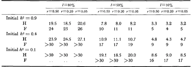
TABLE 3

Half-life and full-life of the additiue genetic variance in different populations

under the additive x additive model

I=80% I=50% z=10%

r T 0 . 5 0 r Z 0 . 2 0 r z 0 . 0 5 r z 0 . 5 0 r=0.20 r z 0 . 0 5 r z 0 . 5 0 r x 0 . 2 0 r x 0 . 0 5

Initial h* = 0.9

H 19.5 18.5 20.6 7.8 8.0 8.2 3.3 3.2 3.2 F 24 23 26 10 1 1 1 1 5 4 5

H 23.9 24.5 27.1 10.9 1 1 . 1 10.7 4.8 4.3 4.7

F >30 >30 >30 1 7 17 19 9 9 9

H >30 >30 >30 19.1 18.5 20.0 8.6 9.0 8.5 F . . . . . . >30 >30 >30 16 17 17

Initial h2 = 0.4

Initial h2 = 0.1

SIMULATED SELECTION

TABLE 4

Half life and full life of the additive genetic variance in different populations under the additive

+

Dominance

+

Epistatic model

85

I=80% r z 0 . 5 0 r=0.20 r z 0 . 0 5

Initial h? = 0.9 H

F

H F

H F Initial h' = 0.4

Initial h' = 0.1

10.7 10.9 7.6 >30 29 >30

14.8 14.9 16.0 >30 >30 >30

28.9 27.5 >30 >30 >30 .

I=50% I=10%

r z O . 5 0 r=0.20 r x 0 . 0 5 r z 0 . 5 0 r=0.20 r=O.O5

1.4 1.6 1.5 4.2 4.2 3.6

14 14 19 12 12 17

6.2 5.9 5.3 2.5 2.7 2.4

>30 27 >30 22 22 18

12.2 11.1 11.4 5.1 5.3 4.8

>30 >30 >30 >30 >30 >30

Consider two loci X and

Y

with two alternative alleles in each locus, A and a

for locus X, B and b for locus Y. The frequency of A is p , and of a is q ( p

+

q = l ) , the frequency of B being r and of b, t ( r

+

t = 1 )

.

If loci

X

and

Y

were showing the A x A interaction, with genetic values of AABB = 8, AaBB =

4

etc. as used in the present study, it can be shown that when

X

and Yare not linked, the addi- tive genetic variance of the population is

32 p 2 r2 (q+t)

UA' =

P4

+

rt

The stationary value of uA2 for values of p and r can be investigated by calculating

a

uA2/ap = 0 and

a

uA2/ar = 0 and solving the two simultaneous equations. The results of partial differentiations were

2 ( p q + r t ) ( l - 2 p + t ) - p ( q + t ) ( l - 2 p )

= o

(1)

2 ( r t

+

p q ) (1 - 2r

+

q ) - r ( t

+

q ) (1 - 2 r ) = 0 ( 2 )

The equations have a solution when p = r. When p = r

04' = 64 p39,

which turns out to be an equation for minimum values of uAi2 for various p values. From among the minimum values the maximum is reached when p = 0.75. In this case each pair of loci will contribute 6.75 units to the additive genetic variance and the total uA2 at the maximum-minimum value will be 33.75. Since gene frequencies for each pair of loci were set at p = r = 0.5 at the beginning of selec- tion, it is therefore not surprising that there was an increase in ai2 after a few generations of selection in each population.

A point worthy of note is that when selection presure was high, the increase in

u . ~ ~ under selection was less than when pressure was low; under high pressure

86 S. S. Y. YOUNG

the frequencies of the favoured genes at a greater speed towards fixation, so that there was insufficient time available for the formation of a n optimal combination of gene frequencies for higher uA2. This situation would be further enhanced if the gene frequencies for the loci were set at the minimum condition of p = I, as in

the present study. Conversely at low selection pressure, relatively more time was available for the formation of favourable combinations of gene frequencies by crossing over.

The increase in uA2 in the initial generations of selection for A

x

A, compared

yVith the consistent decrease in the same variance f o r A and

D,

plus the nonlinear changes in uA2 with selection shown in this study, support two obvious conclusions which have been much discussed but for which there has been little previous data:

(1) There is no reason to expect similar changes in genetic parameters for any two traits of the same organism, under similar selection pressure. (2) It is not surprising to find a difference in rate of change in genetic parameters and a differ- ence in rate of gain for the same character in two populations under similar selection pressure.

If

we accept the above as reasonable then the desirability of estimating genetic parameters as often as possible during selection cannot be denied.

The results also show that h2 is a relatively poor predictor of genetic gain when genes are epistatic or when some of the genes involved show epistatic interaction, even though the epistatic effect assumed here was a relatively simple one. One could imagine under more complex situations, such as the double peaked condi- tional A X A used by GILL (1965a) or with A

x

D

o r

D

x

D

models, the predictive ability of hz might be even poorer. I t is well established in quantitative genetics that when

h2

is low or when mass selection produces no appreciable advance, then greater genetic gain might be obtained by using techniques such as family selec- tion, crossing of inbred lines and so on. I n view of the present conclusions from the A X A and mixed models, it seems worthwhile to propose that when accurate estimates of h2 have failed to predict gains adequately then it may also be worth- while to consider breeding methods for the exploitation of the non-additive genetic variations for greater rate of gain, without waiting for a plateau to be reached. With the present population size of 1000 individuals, genetic drift was found to be unimportant in the results of simulated selection under various genetic models. For the same population tightness of linkage, at least for the levels of recombination probabilities assumed, had no effect on selection limits and had a negligible effect on the rate of change in genetic variances. These findings are in contrast to the results of earlier studies by FRASER (1 95 7)

,

MARTIN and COCKER-

HAM (1960) and GILL (1965) in small populations of 20 to 40 individuals. In

designing selection experiments, it would be valuable to have some knowledge of the minimum size of population in which both linkage and drift would be expected to have only negligible effects on selection results. Further investigation in this area, using the high speed computer, seems to be warranted.

SIMULATED SELECTION 87

this project and to the Department for the facilities they made available to me. Thanks are also due to MISSES E. SMITH, J. STRACHAN and B. FORBES for assistance in the tabulation of the results and to MISS H. NEWTON TURNER for comments on the manuscript. The cost of computation was borne by the U.S. Atomic Energy Commission contract AT(30-1) -2620.

SUMMARY

Genetic advances under truncation selection were simulated. It was assumed that the character under selection was controlled by ten loci, the size of each unselected population being 1000 individuals per generation. Different levels of selection intensities, initial heritabilities and recombination probabilities were incorporated in seven genetic models.-In an earlier paper the results for the additive

(A) and dominance

(D) models were reported. In this paper the results obtained assuming an additive x additive epistatic

(E)

model are discussed to- gether with those for the A

+

D, A

+

E, D

+

E and A

+

D

+

E mixed models.- With the E model, predictions of genetic gains were underestimated when selec- tion pressures were high or intermediate. The predictive ability of h' when mixed models were used varied with the model under consideration: for the A

+

D model predictions were almost as accurate as for the A model, but were erratic for any mixed models involving epistasis. Predictions tended to be more inaccurate as mixed models, involving some epistasis, became more complex.-With the E

model, as well as with mixed models involving some epistasis, the additive genetic variance under the present conditions always increased after initial generations of selection. This is in contrast to results obtained for the A and

D

models under identical conditions. A direct consequence of this was the longer half and full lives of the additive genetic variance calculated for models involving epistatic loci.-Tightness of linkage had no appreciable effects on the predictive ability of h', the ultimate genetic advance and the decay of genetic variances.

LITERATURE CITED

FRASER, A. S., 1957 Simulation of genetic systems by automatic digital computers. I. Introduc- tion. 11. Effects of linkage on rates of advance under selection. Australian J. Biol. Sci. 10: 484-491, 492-499.

-

1960 Simulation of genetic systems by automatic digital com- puters. VI. Epistasis. Australian J. Biol. Sci. 13: 150-162.

A Monte Carlo evaluation of predicted selection response. Australian J. Biol. Sci. 18: 999-1007.

-

196% Effects of finite size on selection advance in simulated genetic populations. Australian J. Biol. Sci. 18: 599-617.

phenotype. Australian J. Biol. Sci. 13: 307-343.

estimating heritability of characters. Am. Soc. Anim. Prod. Proc. 1940, 293-301.

metrical Genetics. Edited by 0 . KEMPTHORNE. Pergamon Press, London. GILL, J. L., 1965a

GRIFFING, B., 1960 Theoretical consequences of truncation selection based on the individual

LUSH, J. L., 1940

MARTIN, F. G., JR., and C. C. COCKERHAM, 1960

YOUNG, S. S. Y., 1966

Intra-sire correlations and regressions of offspring on dam as a method of

High speed selection studies pp. 35-45. Bio-