Generalized Aggregation of Sparse Coded Multi-spectral for Satellite Scene Classification

(1)

Generalized Aggregation of Sparse Coded Multi-spectral

for Satellite Scene Classification

Xian-Hua Han1,*,†and Yen-Wei Chen2

1 _{Yamaguchi University, 1677-1 Yoshida, Yamaguchi City, Yamaguchi 753-8511, Japan}

2 _{Ritsumeikan University, 1-1-1 Nojihigashi, Kusatsu 525-8577, Japan; [email protected]}

* Correspondence: [email protected]; Tel.: +81-083-933-5693

† Current address: Yamaguchi University, 1677-1 Yoshida, Yamaguchi City, Yamaguchi 753-8511, Japan

Abstract:Satellite scene classification is challenging because of the high variability inherent in satellite data. Although rapid progress in remote sensing techniques has been witnessed in recent years, the resolution of the available satellite images remains limited compared with the general images acquired using a common camera. On the other hand, a satellite image usually has a greater number of spectral bands than a general image, thereby permitting the multi-spectral analysis of different land materials and promoting low-resolution satellite scene recognition. This study advocates multi-spectral analysis and explores the middle-level statistics of spectral information for satellite scene representation instead of using spatial analysis. This approach is widely utilized in general image and natural scene classification and achieved promising recognition performance for different applications. The proposed multi-spectral analysis firstly learns the multi-spectral prototypes (codebook) for representing any pixel-wise spectral data, and then based on the learned codebook, a sparse coded spectral vector can be obtained with machine learning techniques. Furthermore, in order to combine the set of coded spectral vectors in a satellite scene image, we propose a hybrid aggregation (pooling) approach, instead of conventional averaging and max pooling, which includes the benefits of the two existing methods but avoids extremely noisy coded values. Experiments on three satellite datasets validated that the performance of our proposed approach is much more accurate than even the deep learning framework for spatial analysis.

Keywords: multi-spectral analysis; remote sensing images; sparse coding; generalized aggregation; scene recognition

1. Introduction

The rapid progress in remote sensing imaging techniques over the past decade has produced an explosive amount of remote sensing (RS) satellite images with different spatial resolutions and spectral coverage. This allows us to potentially study the ground surface of the earth in greater detail. However, it remains extremely challenging to extract useful information from the large number of diverse and unstructured raw satellite images for specific purposes such as land resource management and urban planning [1–4]. Understanding the land on earth using the satellite images generally requires the extraction of a small sub-region of RS images for analysis and for exploring the semantic category. The fundamental procedure of classifying satellite images into semantic categories firstly involves extracting the effective feature for image representation, and then constructing a classification model by using manually annotated labels and the corresponding satellite images. The success of the bag-of-visual-words (BOW) model [5–7] and its extensions for general object and natural scene classification has resulted in the widespread application of these models for solving the semantic category classification problem in the remote sensing community. The BOW model was originally developed for text analysis, and was then adapted to represent images by the frequency of "visual words" that are generally learned from the pre-extracted local features from images by a clustering method (K-means) [5]. In order to reduce the reconstruction error led by approximating a local feature with only one "visual word" in K-means, several variant coding methods such as sparse coding (Sc), Linear Locality-constrained Coordinate (LLC) [8–11], and the Gaussian Mixture Model (GMM) [12–15] have been explored in the BOW model for improving the reconstruction accuracy of local features, and some researchers further endeavored to integrate the spatial relationships of the local features. On the other hand, local features such as SIFT [16], which is handcrafted and designed as a

(2)

gradient-weighted orientation histogram, are generally utilized, and remain untouched in term of their strong effect on the performance of these BOW-based methods [17–19]. Therefore, some researchers investigated the local feature learning procedure automatically from a large number of unlabeled RS images via unsupervised learning techniques instead of using the handcrafted local feature extraction [20–22], thereby improving the classification performance to some extent. Recently, deep learning frameworks have witnessed significant success in general object and natural scene understanding [23–25], and have also been applied to remote sensing image classification [26–31]. These framework perform impressively compared with the traditional BOW model. All of the above-mentioned algorithms firstly explore the spatial structure for providing the local features, which is important for local structure analysis in high-definition general images such as those in which a single pixel covers several centimeters or millimeters. However, the available satellite images are usually acquired at a ground sample distance of several meters, e.g., 30 meters for Landsat 8 and 1 meter even for high-definition satellite images from the National Agriculture Imagery Program (NAIP) dataset [32]. Thus, the spatial resolution of a satellite image is much lower than that of a general image, and the spatial analysis of nearby pixels, which often belong to different categories in a satellite image may not be suitable.

(3)

……

…

Multi-spectral of pixels

…

Spectral prototypes (Endmembers)

Over-complete endmember learning using

clustering method

Multi-spectral

Sparse coded spectral vectors

……

Aggregation of the coded Hybrid spectral vector

for image representation

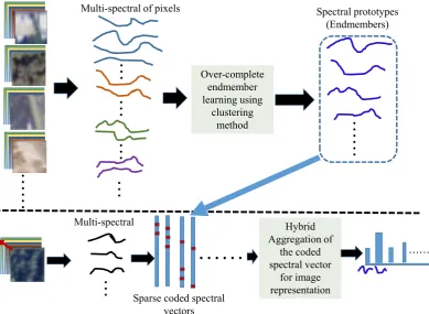
Figure 1.Proposed satellite image representation framework. The top row manifests the learning procedure of the multi-spectral prototypes, whereas the bottom row denotes the coding and pooling procedure of the pixel-wise multi-spectral in images to provide the final representation vector.

combines the popularly applied average and max pooling methods and, rather than awfully emphasizing the maximum activation, preferring a group of activations in the explored region instead. The proposed satellite image representation framework is shown in Fig. 1, where the top row is for over-complete spectral prototype set learning, and the bottom row manifests the sparse coding of any pixel spectral and the hybrid pooling strategy of all coded spectral vectors in a sub-region to form discriminated feature.

The main contributions of our work are threefold: (1) Because of the low spatial resolution of satellite images, we first explore spectral analysis instead of spatial analysis, which is widely used in general object and natural scene recognition. (2) Unlike the spectral analysis in the unmixing model, which usually only obtains the sub-complete basis (the number of the bases are fewer than the number of spectral bands) via simplex identification approaches, we investigate the over-complete dictionary for more accurate reconstruction of any pixel spectrum, and obtain the reconstruction coefficients by using a sparse coding technique; (3) We generate the final representation of a satellite image from all coded sparse spectral vectors, for which we propose a generalized aggregation strategy. This strategy not only integrates the maximum magnitude but also the response magnitude of the relatively large coded coefficients of a specific spectral prototype instead of employing the conventional max and average pooling approaches.

(4)

2. Related work

Considerable research efforts are being devoted to understanding satellite images. Among the approaches researchers have developed, the bag-of-visual-words (BOW) model [5–7] and its extensions have been widely applied to land-use scene classification. In general, this type of classification considers large scale categories (with coverage of tens or hundreds of meters in one direction) such as airports, farmland, ports, and parks. A flowchart of the BOW model is shown in Fig. 2, and includes the following three main steps: 1) Local descriptor extraction, which concentrates to explore the spatial relation of nearby pixel and ignores or separately analyzes the intensity variation of different colors (spectral bands) by using methods such as SIFT [16] and SURF [40]; 2) A coding procedure, which approximates a local feature using a linear combination of pre-defined or learned bases (codebook), and transforms each local feature into a more discriminated coefficient vector; 3) A pooling step, which aggregate all the coded coefficient vectors in region of interest into the final representation of this region via a max or average pooling strategy. The local descriptor in the BOW model for most applications usually remains untouched as SIFT and SURF, of which the design is handcrafted for exploring the local distinctive structure of the target objects. The local descriptor, which is most generally used, namely SIFT, needs to roughly and uniformly quantize the gradient direction between the nearby pixels into several orientation bins; however this would cause loss of some subtle structures and affect the final image representation ability. Therefore, some researchers investigated the local feature extraction procedure by automatically learning from a large number of unlabeled images with unsupervised learning techniques instead of using the handcrafted local feature extraction [20–22], and improved the classification performance to some extent. However, all of the above-mentioned algorithms mainly concentrate on spatial analysis to explore the distinctive local structure of general objects, and take less consideration of the color (spectral) information, an approach would be unsuitable for satellite scene classification as a result of its low spatial resolution. Recently developments in deep convolutional networks have witnessed their great success in different image classification applications, including applications involving the use of remote sensing images; however these methods still focus on convoluting a spatial supported region into local feature maps. Because of the presence of multiple available spectral bands in satellite images, this study proposes to investigate the pixel spectral band and validate the feasibility and effectiveness for satellite scene classification.

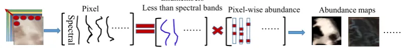
On the other hand, the existence of multiple spectral bands (also known as hyper-spectral data) in satellite images has promoted many researchers to propose pixel-wise land cover investigation to enable the variety of mixed pixels, known as an unmixing model [33–35], to be processed. The purpose of the unmixing model is to decompose the raw satellite images, composed of mixed pixels, into several material composition fraction maps and the corresponding set of pure spectral materials (also known as endmembers). The flowchart representing this procedure is shown in Fig. 3. Given a multi-spectral satellite imageIwith sizeB∗N∗M(whereBdenotes the number of spectral bands, andNandMdenote the height and width of the satellite image, respectively), where the pixels may cover several types of land materials due to the low spatial resolution, we first re-arrange the image in the form of a matrixZwith a pixel-wise spectral column vector (size: B∗(N∗M)). The spectral vector ziof theithpixel is assumed to be a linear combination of several endmembers (basis) with the composition

fraction as the weighted coefficients:zi=Eai, whereE= [e1,e2,· · ·,eK]is a set of spectral column vectors

(K) representing the existing endmembers (land materials) in the processed satellite image. Considering the physical phenomenon of the spectral image, the elements in the endmember spectral and the fraction magnitude of the pixel abundance are non-negative, and the abundance vector for each pixel is summed to one. Then, the matrix formula for all pixels in a satellite image of interest can be formed as follows:

Z=EA,s.t.E>=0,A>=0,

∑

ai =1 (1)

(5)

Key-points with support region

……

Spatial Analysis

Local descriptors

…… Coding

: Prototypes (basis): local descriptors

……

Pooling Final Representation

Sp

ect

ral ……

Pixel Abundance maps

……

Pixel-wise abundance

…… _……

Endmembers Less than spectral bands

Figure 2.Bag-of-Visual-words model for image representation.

Key-points with support region

…… Spatial

Analysis

Local descriptors

…… Coding

: Prototypes (basis): local descriptors

……

Pooling Final Representation

Sp

ect

ral ……

Pixel Abundance maps

……

Pixel-wise abundance

…… _……

Endmembers Less than spectral bands

Figure 3.Flowchart of the linear unmixing model.

images, and an over-complete dictionary is preferred to take into consideration the variety of pixels in the same material and possible outliers in the target application. In the next section, we describe our proposed strategy in detail.

3. Generalized Aggregation of Sparse Coded Multi-spectral

The low spatial resolution of satellite images, for example a30×30ground sampling distance of each pixel in LandSat 8 images, has led us to focus on the multiple spectral bands of a single pixel for statistical analysis. LetXbe the set ofD-dimensional spectral vectors of all pixels extracted from a satellite image, i.e. X= [x1,x2,· · ·,xN]∈RD×N. Our goal is first to code the spectral vector to a more discriminated coefficient vector based on a set of common bases (codebook). Given a codebook withKentries,B= [b1,b2,· · ·,bK]∈

RD×K, different coding schemes can transform each spectral into an K-dimensional coded coefficient vector to generate the final image representation. Next, we provide the detail of the codebook (an over-complete basis) learning and coding methods.

3.1. Codebook learning and spectral coding approaches

The most widely applied codebook learning and vector coding strategy in general object recognition applications is the vector quantization (VQ) method. However, because this strategy approximates any input vector with only one learned base, it possibly leads to a large reconstruction error. Therefore, several efforts have been made to approximate an input vector using a linear combination of several bases such as sparse coding (SC) and locality-constrained linear coding (LLC). These methods have been proven to perform impressively in different general object and natural scene classifications. As mentioned in [11], smoothness of coded coefficient vectors is more important than the sparse constraint. This means the coded coefficient vector should be similar if the inputs are similar. Therefore, this study focuses on locality-constrained sparse coding for multi-spectral analysis.

Vector quantization: given training samplesX= [x1,x2,· · ·,xN], the codebook learning procedure with

VQ solves the following constrained least-squares fitting problem:

min B,C

N

∑

n=1

kxn−Bcnk2

subject to: Card(cn) =1,kcnk1=1;ci≥0;

(2)

whereC= [c1,c2,· · ·,cN]is the set of codes forX. The cardinality constraintCard(ci) =1means that

(6)

constraintci ≥0and sum-to-one constraintkcik1=1means that the summation of the coded weight forxiis 1.

The codebookB= [b1,b2,· · ·,bK]can be learned from the prepared training samples, which are the spectral

vectors of all pixels from a large number of satellite images, by the Expectation Maximization (EM) strategy. The detail agorithm of the VQ implementation in Eq. (2) is shown inAlgorithm1. In the VQ method, the codebook vectors can be freely assigned as any larger number than the dimension of the input spectral vectorxn, which

forms an over-complete dictionary. After learning the codebook using the training spectral samples, it is fixed for coding the multi-spectral vectors of all pixels. The VQ approach can obtain the sparsest representation vector cnfor an input vectorxn (only one non-zero value), which means that it only approximates any input vector

with one selected base from the codebookBand thus leads to large reconstruction error. Therefore, several researchers proposed to the use of sparse coding for vector coding, which can adaptively select several bases to approximate the input vector and thus reduce the reconstruction error. Sparse coding has been proven to perform more effectively in different applications.

Locality-Constrained Sparse Coding: In terms of local coordinate coding, Wang et al. [11] claimed that locality is more important than sparsity, which not only leads to sparse representation but also retains the smoothness between the transformed representation space and the input space. Therefore, this study incorporates a locality constraint instead of the pure sparsity constraint in Eq.(3). This approach can simultaneously result in sparse representation, known as the locality locality-constraint sparse coding (LcSC), which is applied for codebook learning and spectral coding with the following criteria:

min B,C

N

∑

n=1

kxn−Bcnk2+λksncnk2

subject to: 1Tcn=1,∀n;

(3)

where the first term is the reconstruction error for the used samples and the second term is the constraint of locality and implicit sparsity.denotes the element-wise multiplication, and the constraint1Tcn =1allows the

shift-invariant codes.sn∈RDis the locality controller for supplying different freedom of each basis vectorbk

proportional to its similarity to the input descriptorxn. We define the controller vectorsnas the following:

sn= [sn1,sn2,· · ·,snK]

= [exp(kxn−b1k2

σ ),· · ·,exp(

kxn−bKk2

σ )]

(4)

whereσis used for adjusting the rate of weight decay for the locality controller. The locality controller vector

imposes very large weight on the coded coefficients of the basis vectors that have no similarity (large distance) to the input vector, and in the results the coefficients corresponding to the basis vectors that are not similar would be extremely small or zero. Therefore, the resulting coded vector for any inputxnwould be sparse and smooth

between the coded space and the input space as a consequence of only using similar basis vectors. The detail implementation of the LcSC method in Eq. (3) is shown inAlgorithm2.BinitinAlgorithm2 is initialized with

the VQ method.

Algorithm 1Codebook learning of VQ method in Eq. (2).

Input:X∈RD×N Output:B

Initialization:Randomly takeKsamplesBinit ∈RD×KfromXfor initializingB:B←Binit.

2: forn=1 :Ndo fork=1 :Kdo

4: Calculate the Euclidean distancednkbetweenxnandbk, and assign

xntok0−thcluster ifdnk0 =min_k(d_nk), end for

6: Recalculatebkwith the assigned samplesXkto thekthcluster

end for

(7)

Algorithm 2Codebook learning of LcSC method in Eq. (3).

Input:Binit ∈RD×K,X∈RD×N,λ,σ

Output:B

1: Initialization:B←Binit.

2: forn=1 :Ndo 3: fork=1 :Kdo

4: Calculate the control elementsnkbetweenxnandbkusing Eq. (4),

5: end for

6: Normalizedn:dn←normalize(0,1)(dn);

7: Calculate the temporary coded vectorcnwith the fixed codebookBusing Eq. (3),

8: Refine the coded vectorcnvia selecting the atoms with the larger coded coefficients only:

id← {k|abs(cn(k)>0.01},Bn←B(:,id), and

c0n←minckxn−Bncnk2,s.t.∑kc0n(k) =1.

9: UpdateBn:Bn←Bn−µ4Bn/|c0n|2, whereBn=−2c0n(xn−Bnc0n)andµ=

√ 1/n, 10: ProjectBnback toB:B(:,id)←proj(Bn)

11: end for

3.2. Generalized Aggregation Approach

Given a satellite image sub-region, the multi-spectral vectorsX= [x1,x2,· · ·,xN]having the same number

of pixels can be generated, and thus produce the same number of coded coefficient vectorsC= [c1,c2,· · ·,cN]

using coding approaches. The approach selected to aggregate the obtained coefficient vectors to form the final representationzof the investigated sub-region plays an essential role in determining the recognition results of this region. As we know, the widely used pooling methods for aggregating the encoded coefficient vectors in the traditional BOW model and its extension versions are average and max strategies. Average pooling aggregates all the weighted coefficients, which are the coded coefficients of a pre-learned word in the BOW model, in a defined region by taking the average value, whereas max pooling aggregates these by taking the maximum value. In the vision community, the max pooling in combination with popularly used coding methods such as SC and soft assignment manifests promising performance in a variety of image classification applications. However, the max-pooling strategy only retains the strongest activated pattern (the learned visual word), and would completely ignore the frequency of the activated patterns (visual words). This frequency counting the number of local descriptors, which are similar to the learned visual words, is also an important signature for identifying different types of images. Therefore, this study proposes a hybrid aggregation (pooling) strategy of the sparse coded spectral vectors by integrating not only the maximum magnitude but also the response magnitude of the relatively large coded coefficients of a specific spectral prototype, termed K-support pooling. This proposed hybrid pooling strategy combines the popularly used average- and max- pooling methods and can avoid emphasizing the maximum activation, instead, it prefers using a group of activations in the explored region.

Let us denote the coded coefficient weight of thekthcodebook vector for thenthmulti-spectral in a satellite imageIasck,n. We aim to aggregate all the coded weights of thekthcodebook vector in the imageIto obtain

the overall weight indication as the following:

zI_k= f({ck,n},n∈I) (5)

wherezI

kdenotes the pooled coded weight of of thekthcodebook vector in the imageI. We can design different

transformation function f for aggregating the set of activations into a indicating value. The simplest pooling method simply averages the coded weights of all input vectors in this processed image formulated as:

zI_k= 1

NI_n

∑

∈I

ck,n (6)

(8)

maximum activation would be more related to the human cortex response than the average activation, and can provide translation-invariant visual representation. Therefore, the max pooling strategy has been widely used accompanied with SC and soft assignment coding strategies in the BOW model. The max-pooling can be formulated as:

zI_k=maxck,n({ck,n},j∈I)

=ck,l,ck,l>=ck,n,l6=n,l,n∈I

(7)

Max pooling takes the maximum coded weights of all input vectors in an images as the overall activation degree, and then completely ignores how many inputs are possibly activated. This study proposes a hybrid aggregation (pooling) strategy of the sparse coded spectral vectors by integrating not only the maximum magnitude but also the response magnitude of the relatively large coded coefficients of a specific spectral prototype. The resulting integration is named K-support pooling. The proposed generalized aggregation approach firstly sorts the coefficient weight of thekthcodebook vector of all inputs from large to small values in a processed imageIas:

c0_k_,_n =sort{ck,n},

withc0_k_,1>=c0_k_,2>=c0_k_,3>=· · ·>=c0_k_,_N

I,n∈I

(8)

and then only retains the first L larger coefficient weights. The final activation degree of the processed prototype is calculated by averaging the retained L-values, which is the mean of the selected L-support locations (pixels), named as K-support pooling. It is formulated as the following:

zI_k= 1

L

∑

c 0

k,n (9)

For each codebook vector, we repeat the above procedure, and produce the activation degrees of all codebook vectors in a processed image. Finally, the L aggregated coefficient weights can be obtained for representing the processed image.

4. Experiments

4.1. Datasets

(9)

(a)Sample images from SAT-4 dataset

(b)Sample images from SAT-6 dataset

Figure 4.Some sample images. (a) Sample images from the SAT-4 dataset. Each row denotes a class of images, and from top to bottom the classes are barren land, trees, grassland and others, respectively. (b) Sample images from the SAT-6 dataset. Each row denotes a class of images, and from top to bottom the classes are buildings, barren land, trees, grassland, roads and water bodies, respectively.

0

20

40

60

80

100

120

140

160

180

200 MSP1

MSP2

MSP3

MSP4

(10)

1 0.8 0.6 0.4 0.2 0 1 0.8 0.6 0.4 0.2 0 1 0.8 0.6 0.4 0.2 0 1 0.8 0.6 0.4 0.2 0

<0.025 <0.075 <0.125 <0.175 <0.225 <0.275 >0.275 <0.025 <0.075 <0.125 <0.175 <0.225 <0.275 >0.275

<0.025 <0.075 <0.125 <0.175 <0.225 <0.275 >0.275 <0.025 <0.075 <0.125 <0.175 <0.225 <0.275 >0.275 Barren land Trees Grassland Others Barren land Trees Grassland Others Barren land Trees Grassland Others Barren land Trees Grassland Others 1 0.8 0.6 0.4 0.2 0 1 0.8 0.6 0.4 0.2 0 1 0.8 0.6 0.4 0.2 0 1 0.8 0.6 0.4 0.2 0

<0.025 <0.075 <0.125 <0.175 <0.225 <0.275 >0.275 <0.025 <0.075 <0.125 <0.175 <0.225 <0.275 >0.275

<0.025 <0.075 <0.125 <0.175 <0.225 <0.275 >0.275 <0.025 <0.075 <0.125 <0.175 <0.225 <0.275 >0.275 Barren land Trees Grassland Others Barren land Trees Grassland Others Barren land Trees Grassland Others Barren land Trees Grassland Others (a) For MSP1 in Fig.5. (b) For MSP2 in Fig.5. 1 0.8 0.6 0.4 0.2 0 1 0.8 0.6 0.4 0.2 0 1 0.8 0.6 0.4 0.2 0 1 0.8 0.6 0.4 0.2 0

<0.025 <0.075 <0.125 <0.175 <0.225 <0.275 >0.275 <0.025 <0.075 <0.125 <0.175 <0.225 <0.275 >0.275

<0.025 <0.075 <0.125 <0.175 <0.225 <0.275 >0.275 <0.025 <0.075 <0.125 <0.175 <0.225 <0.275 >0.275 Barren land Trees Grassland Others Barren land Trees Grassland Others Barren land Trees Grassland Others Barren land Trees Grassland Others 1 0.8 0.6 0.4 0.2 0 1 0.8 0.6 0.4 0.2 0 1 0.8 0.6 0.4 0.2 0 1 0.8 0.6 0.4 0.2 0

<0.025 <0.075 <0.125 <0.175 <0.225 <0.275 >0.275 <0.025 <0.075 <0.125 <0.175 <0.225 <0.275 >0.275

<0.025 <0.075 <0.125 <0.175 <0.225 <0.275 >0.275 <0.025 <0.075 <0.125 <0.175 <0.225 <0.275 >0.275 Barren land Trees Grassland Others Barren land Trees Grassland Others Barren land Trees Grassland Others Barren land Trees Grassland Others

(c) For MSP3 in Fig.5. (d) For MSP4 in Fig.5.

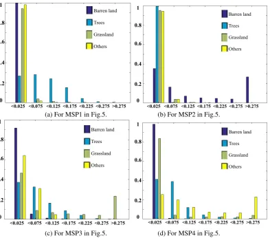
Figure 6.Image number statistics of the aggregated coefficients for different learned multi-spectral prototypes and the SAT-4 training dataset. (a) The image frequency of different land use classes between different aggregated coefficient regions of the MSP1 in Fig. 5; (b) For the MSP2 in Fig. 5; (b) For the MSP3 in Fig. 5; (b) For the MSP4 in Fig. 5.

recognition performance for the SAT-4 and SAT-6 datasets. We compare the recognition performance using our proposed spectral analysis framework and state-of-the-arts based on deep learning techniques in experimental results subsection.

In addition, we constructed a Megasolar dataset [?], which was collected from 20 satellite images taken in Japan, 2015, by Landsat 8. The used image have 7 channels corresponding to different wavelengths, where half are correspond to the non-visible infra-red spectrum, and their resolution is of roughly 30 meters per pixel. The satellite images are divided into16×16cells; more than 20%of the pixels covered by a power plant are considered as positive samples, while those without a single pixel belonging to a power plant are treated as negative samples. There are 300 training positive samples augmenting to 4851 by rotation transformation, and 2,247,428 training negative samples. The positive samples in validation and test subset are 126, and the negative samples are more than 860,000. In our experiments, we exploited the augmented 4851 positive samples and randomly selected 4851 negative samples from training subset for training, and the 126 positive samples in validation and test subsets and randomly selected 3000 negative samples are for test.

4.2. Spectral Analysis

(11)

94 95 96 97 98 99 100 SAT-4

SAT-6

Recognition Accuracy (%)

K=512 K=256 K=128 K=64 K=32

Figure 7.Recognition accuracies of the proposed multi-spectral representation based on the VQ coding strategy under different codebook sizes (K=32, 64, 128, 256, 512) for both datasets SAT_4 and SAT_6.

95 95.5 96 96.5 97 97.5 98 98.5

LcSC_max LcSC_L50 LcSC_L100 LcSC_Ave

K=64: Recognition accuracy (%)

SAT-4 SAT-6 97 97.5 98 98.5 99

SAT-4 SAT-6 98.4 98.6 98.8 99 99.2 99.4

SAT-4 SAT-6 99.1 99.2 99.3 99.4 99.5 99.6 99.7 99.8

SAT-4 SAT-6 95 95.5 96 96.5 97 97.5 98 98.5

SAT-4 SAT-6 97 97.5 98 98.5 99

SAT-4 SAT-6 98.4 98.6 98.8 99 99.2 99.4

SAT-4 SAT-6 99.1 99.2 99.3 99.4 99.5 99.6 99.7 99.8

SAT-4 SAT-6 (a)Codebook size: K=64 (b) Codebook size: K=64 95 95.5 96 96.5 97 97.5 98 98.5

SAT-4 SAT-6 97 97.5 98 98.5 99

SAT-4 SAT-6 98.4 98.6 98.8 99 99.2 99.4

SAT-4 SAT-6 99.1 99.2 99.3 99.4 99.5 99.6 99.7 99.8

SAT-4 SAT-6 95 95.5 96 96.5 97 97.5 98 98.5

SAT-4 SAT-6 97 97.5 98 98.5 99

SAT-4 SAT-6 98.4 98.6 98.8 99 99.2 99.4

SAT-4 SAT-6 99.1 99.2 99.3 99.4 99.5 99.6 99.7 99.8

SAT-4 SAT-6

(c)Codebook size: K=256 (d) Codebook size: K=512

(12)

99.1 99.2 99.3 99.4 99.5 99.6 99.7 99.8

SAT-4 SAT-6

VQ_Ave LcSC_Ave LcSC_GP

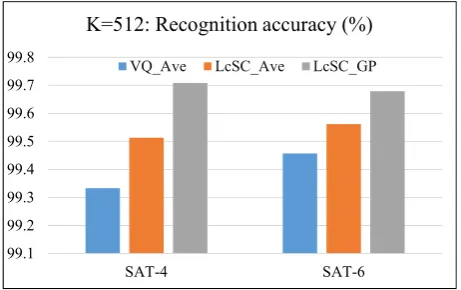
Figure 9.Compared recognition accuracies based on VQ and LcSC coding strategies for codebook size:K=512 for both datasets SAT-4 and SAT-6.

Table 1.Confusion matrix using LcSC coding and the proposed generalized pooling strategy with codebook size K=512 for both SAT-4 and SAT-6 datasets.

(%) Barren land Trees Grassland Others

Barren land 99.404 0 0.554 0.042

Trees (linear) 0 99.97 0.035 0

Grassland 0.407 0.061 99.515 0.017

Others 0.034 0.003 0.003 99.961

(a) SAT-4

(%) Building Barren land Trees Grassland Road Water

Building 100 0 0 0 0 0

Barren land 0 99.134 0 0.866 0 0

Trees 0 0 99.894 0.106 0 0

Grassland 0.008 0.802 0.143 99.047 0 0

Road 0 0 0 0 100 0

Water 0 0 0 0 0 100

(b) SAT-6

(13)

Table 2.Compared overall accuracies on SAT-4 and SAT-6 datasets with DeepSat(Basu et al., 2015) [29,30] and DCNN (Ma et al., 2016) [31].

Methods SAT-4 SAT-6

DBN [Basu et al., 2015] 81.78 76.41

CNN [Basu et al., 2015] 86.83 79.06

SDAE [Basu et al., 2015] 79.98 78.43

Semi-supervised [Basu et al., 2015] 97.95 93.92

DCNN [Ma et al., 2016] 98.408 96.037

Ours 99.709 99.679

4.3. Experimental Results

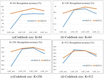
In this section, we evaluate the recognition performance on the SAT-4, SAT-6 and Megasolor datasets using our proposed multi-spectral analysis. With the aggregated coded spectral vector, we simply use a linear SVM as classifier, which learns the classification model with the images in training dataset, and predicts the land use class label for the images of the test dataset. The recognition performances on SAT-4 and SAT-6 using the VQ coding approach combined with the average pooling strategy and different codebook sizes (K=32, 64, 128, 256, 512) are shown in Fig. 7. The results in this figure confirm recognition performance of approximately 95%on average for both the SAT-4 and SAT-6 datasets even with codebook size 32 only, whereas accuracy of more than 99%is achieved with codebook size 512. Next, we evaluate the recognition performances using the LcSC coding approach with different pooling methods (Average: LcSC_Ave, Max: LcSC_Max, and the proposed generalized method: LcSC_L50, LcSC_L100 with the top 50 and 100 largest weights) and different codebook sizes as shown in Fig. 8(a)-(d). Fig. 8 shows that the proposed generalized pooling method can achieve a more accurate recognition performance than the conventional average- and max-pooling strategies under different codebook sizes. Fig. 9 provides a comparison of different coding strategies (VQ and LcSC) with codebook size 512 on the SAT-4 and SAT-6 datasets. These results confirm the improvement of the proposed coding and pooling strategies. Table 1 contains the confusion matrix using the aggregated sparse coded vector with the LcSC coding and the proposed generalized pooling strategies under codebook size 512, where the recognition accuracies for all land use classes exceed 99%. Finally, the results of the performance comparison with state-of-the-art methods in [29–31] are provided. The comparison involved the application of different kinds of deep frameworks: DBN, DCN SDE, the designed deep architectures in [29,30], named as DeepSat, and DCNN in [31], which integrated the inception module for taking into account the multi-scale variance in satellite images. Table 2 provides the compared average recognition accuracies on both the SAT-4 and SAT-6 datasets, and reveals that our proposed framework achieves the best recognition performance.

In following, the recognition performance on the Megasolar dataset with 7 spectral chanels is provided. The experimental results using the LcSC coding approach with different pooling methods (Average: LcSC_Ave, Max: LcSC_Max, and the proposed generalized method: LcSC_L50, LcSC_L100 with the top 50 and 100 largest weights) and different codebook sizes are given in Fig. 10. Since the unbalance test sample numbers for positive and negative, the average recognition accuracy of the test positive and negative samples are computed, Fig. 10 manifests that the proposed generalized pooling method can achieve a more accurate recognition performance than the conventional average- and max-pooling strategies under different codebook sizes.

4.4. Computational Cost

(14)

90 92 94 96 98 K=32

K=64 K=128 K=256 K=512

LcSC_Ave LcSC_L100 LcSC_L50 LcSC_max

Recognition Accuracy (%)

Figure 10. Recognition accuracies of the proposed multi-spectral representation based on LcSC coding and different pooling strategies under codebook sizes (K=32, 64, 128, 256, 512) for Megasolar dataset.

Table 3. Computational times of different procedures in our proposed strategy. CL, FE, SVM-T and SVM-P denote codebook learning, feature extraction, SVM training and SVM prediction, respectively, while ’s’ and ’m’ represent second and minute, CB size denote codebook size, respectively.

CB size Off-line On-line

CL (s) SVM-T (m) FE (s) SVM-P (s)

SAT-4 SAT-6 SAT-4 SAT-6 For one 28×28 image

Dict:256 270.40 393.17 42.62 9.54 0.024 0.010

Dict:512 530.96 906.17 52.89 11.25 0.038 0.014

steps: feature extraction (FE) and class label prediction with the pre-learned SVM model (SVM-P). Table 3 provides the computational times of different procedures in our proposed strategy with atom numbers: K=256, 512, for both SAT-4 and SAT-6 datasets, where we randomly selected 500 images from each class for codebook learning. From Table 3, it can be seen that the off-line procedures take a little long computational time, while the on-line feature extraction and SVM prediction procedures for one28×28image are really fast with decades millisecond only.

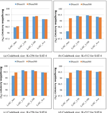
Since the codebook learning for LcSC is an unsupervised procedure, and it may not greatly affect the recognition performance with different numbers of images. We implemented the multi-spectral analysis strategy with the learned codebook using the randomly selected 10 images (denoted as INum10) only, instead of 500 images (denoted as INum500, in the previous experiments) from each class, and provide the compared results in Fig. 11. From Fig. 11 we can see that except the max-pooling based LcSC feature there are no obvious differences in recognition performances with the learned codebook using different image numbers, and thus it can say our proposed feature extraction strategy is robust to codebook learning procedure. The processed time for codebook learning with 10 and 500 images from each class, respectively, for both SAT-4 and SAT-6 datasets are shown in Table 4, which manifests the computational time can be greatly reduced for codebook learning with small number of images.

Table 4.Processed time (s) for codebook learning with 10 and 500 images, respectively, for both SAT-4 and SAT-6 datasets.

codebook size SAT-4 SAT-6

INum10 INum500 INum10 INum500

K=256 4.54 270.40 6.61 393.17

(15)

97.5 98 98.5 99 99.5 100 INum10 INum500 R ec ogn it ion A cc u rac y (%) 97.5 98 98.5 99 99.5 100 INum10 INum500 R ec ogn it ion A cc u rac y (%) 97.5 98 98.5 99 99.5 100 INum10 INum500 R ec ogn it ion A cc u rac y (%) 97.5 98 98.5 99 99.5 100 INum10 INum500 R ec ogn it ion A cc u rac y (%)

(a) Codebook size: K=256 for SAT-4 (b) Codebook size: K=512 for SAT-4 97.5 98 98.5 99 99.5 100 INum10 INum500 R ec ogn it ion A cc u rac y (%) 97.5 98 98.5 99 99.5 100 INum10 INum500 R ec ogn it ion A cc u rac y (%) 97.5 98 98.5 99 99.5 100 INum10 INum500 R ec ogn it ion A cc u rac y (%) 97.5 98 98.5 99 99.5 100 INum10 INum500 R ec ogn it ion A cc u rac y (%)

(c) Codebook size: K=256 for SAT-6 (d) Codebook size: K=512 for SAT-6

Figure 11.Compare recognition accuracies of the proposed multi-spectral representation based on LcSC coding with the learned codebook using 10 and 500 images, respectively, from each class for both SAT-4 and SAT-6 datasets. The compared accuracies with (a) codebook size: K=256 for SAT-4, (b) codebook size: K=512 for SAT-4, (c) codebook size: K=256 for SAT-6, and (d) codebook size: K=512 for SAT-6.

5. Conclusions

(16)

recognition performance of our proposed approach is even superior to that of the deep learning framework for spatial analysis.

References

1. Xu, Y.; Huang, B. Spatial and temporal classification of synthetic satellite imagery: Land cover mapping and accuracy

validation.Geo-spatial Information Science2014,17(1), 1-7.

2. Rogan, J.; Chen, D.M. Remote sensing technology for mapping and monitoring land-cover and land-use change.

Progress in Planning2004,61, 301-325.

3. Jaiswal, R.K.; Saxena, R.; Mukherjee S. Application of remote sensing technology for land use/land cover change

analysis.Journal of the Indian Society of Remote Sensing1999,27(2), 123-128.

4. Xia, G.S.; Yang, W.; Delon, J.; Gousseau, Y.; Sun, H.; Maitre, H. Structrual High-Resolution Satellite Image Indexing.

Proceedings of the ISPRS, TC VII Symposium Part A: 100 Years ISPRS2010, 5-7.

5. Jiang, Y.-G.; Ngo, C.-W.; Yang, J. Towards optimal bag-of-features for object categorization and semantic video

retrieval.Proceedings of the 6th ACM international conference on Image and video retrieval2007, 494-501. 6. Jurie, F.; Triggs, B. Creating efficient codebooks for visual recognition.Proceedings of the Tenth IEEE International

Conference on Computer Vision (ICCV’05)2005,1, 604-610.

7. Jegou, H.; Douze, M.; Schmid, C. Packing bag-of-features.Proceedings of the 12th IEEE International Conference on

Computer Vision (ICCV’09)2009.

8. Lazebnik, S.; Schmid, C.; Ponce, J. Beyond bags of features: spatial pyramid matching for recognizing natural scene

categories.Proceedings of the IEEE Computer Society Conference on Computer Vision (CVPR’06)2006,2, 2169-2178.

9. Yang, J.C.; Yu, K.; Gong, Y.H.; Huang, T. Linear spatial pyramid matching using sparse coding for image classification.

Proceedings of the IEEE Computer Society Conference on Computer Vision (CVPR’09)2009.

10. Yu, K.; Zhang, T.; Gong, Y.H. Nonlinear learning using local coordinate coding.Proceedings of the Advances in Neural Information Processing Systems 22 (NIPS’09)2009, 2223-2231.

11. Wang, J.J.; Yang, J.C.; Yu, K.; Lv, F.J.; Huang, T.; Gong, Y.H. Locality-constrained Linear Coding for Image

Classification.Proceedings of the IEEE Computer Society Conference on Computer Vision (CVPR’10)2010.

12. Han, X.-H.; Chen, Y.-W.; Xu, G. High-Order Statistics of Weber Local Descriptors for Image Representation.IEEE

Transactions on Cybernetics2015,45(6), 1180-1193.

13. Jegou, H.; Douze, M.;Schmid, C. Improving Bag-of-Features for Large Scale Image Search.International Journal of

Computer Vision2010,87(3), 316-336.

14. Perronnin, F.; Sanchez, J.; Mensink. T. Improving the Fisher Kernel for Large-Scale Image Classification.Proceedings

of the 11th European conference on Computer vision (ECCV2010)2010,4, 143-156.

15. Han, X.-H.; Wang, J.; Xu, G.; Chen, Y.-W. High-Order Statistics of Microtexton for HEp-2 Staining Pattern

Classification.IEEE Transactions on Biomedical Engineering2014,61(8), 2223-2234.

16. Lowe, D. G. Distinctive image features from scale-invariant keypoints.IInternational Journal of Computer Vision2004,

60(2), 91-110.

17. Yang, Y.; Newsam, S. Bag-of-visual-words and spatial extensions for land-use classification.Proceedings of the 18th

SIGSPATIAL International Conference on Advances in Geographic Information Systems2010, 270-279.

18. Zhao, L.J., Tang, P.; Huo, L.Z. Land-use scene classification using a concentric circle structured multiscale

bag-of-visual-words model. IEEE Journal f Selected Topics in Applied Earth Observation and Remote Sensing

2014,7(12), 4620-4631.

19. Chen, S.; Tian, Y. Pyramid of Spatial Relations for Scene-Level Land Use Classification. IEEE Transactions on

Geoscience and Remote Sensing2014,53(4), 1947-1957.

20. Cheriyadat, A. Unsupervised Feature Learning for Aerial Scene Classification.IEEE Transactions on Geoscience and

Remote Sensing2014,52(1), 439-451.

21. Zhang, F.;Du, B.; Zhang, L. Saliency-Guided Unsupervised Feature Learning for Scene Classification. IEEE

Transactions on Geoscience and Remote Sensing2015,53(4), 2175-2184.

22. Hu, F.; Xia, G.; Wang, Z.;Huang, X.;Zhang, L.; Sun, H. Unsupervised Feature Learning via Spectral Clustering of

Multidimensional Patches for Remotely Sensed Scene Classification.IEEE Journal of Selected Topics in Applied Earth

Observation and Remote Sensing2015,8(5), 2015-2030.

23. Simonyan, K.; Zisserman, A. Very deep convolutional networks for large-scale image recognition. CoRR2014,

(17)

24. Jia, Y.; Shelhamer, E., Donahue, J.; Karayev, S.; Long, J.; Girshick, R.; Guadarrama, S.; Darrell, T. Caffe: Convolutional

Architecture for Fast Feature Embedding. Proceedings of the 22nd ACM international conference on Multimedia

(MM2014)2014, 675-678.

25. Razavian, A.S.; Azizpour, H.; Sullivan, J.; Carlssonand, S. CNN features off-the-shelf: An astounding baseline for

recognition.Proceedings of IEEE Conference on Computer Vision and Pattern Recognition Workshops2014, 512-519.

26. Castelluccio, M.; Poggi, G.; Sansone, C.; Verdoliva, L. Land Use Classification in Remote Sensing Images by

Convolutional Neural Networks.CoRR2015,abs/1508.00092.

27. Penatti, O.A. B.; Nogueira, K.;Santos, J.A. dos. Do Deep Features Generalize from Everyday Objects to Remote

Sensing and Aerial Scenes Domains?.Proceedings of IEEE Conference on Computer Vision and Pattern Recognition

Workshops2015, 44-51.

28. Hu, F.; Xia, G.; Hu, J.W.; Zhang, L.P. Transferring Deep Convolutional Neural Networks for the Scene Classification of

High-Resolution Remote Sensing Imagery.Remote Sensing2015,7(11), 14680-14707.

29. Basu, S.; Ganguly, S.; Mukhopadhyay, S.; Dibiano, R.; Karki, M.; Nemani, R. DeepSat - A Learning framework

for Satellite Imagery. Proceedings of the 23rd SIGSPATIAL International Conference on Advances in Geographic

Information Systems2015.

30. Basu, S.; Ganguly, S.; Mukhopadhyay, S.; Dibiano, R.; Karki, M.; Nemani, R. DeepSat - A Learning framework for

Satellite Imagery.CoRR2015,abs/1509.03602.

31. Ma, Z.; Wang, Z.P.; Liu, C.X.; Liu, X.Z. Satellite imagery classification based on deep convolution network.

International Journal of Computer, Automation, Control and Information Engineering2016,10(6), 1055-1059.

32. WWW2. NAIP. http://www.fsa.usda.gov/Internet/FSA_File/naip_2009_info_final.pdf.

33. Adams, J.B; Smith, M. O.; Johnson, P.E. Spectral mixture modeling: A new analysis of rock and soil types at the Viking Lander 1 site.Journal of Geophysical Research1986,91(B8), 8098-8112.

34. Settle, J.; Drake, N. Linear mixing and the estimation of ground cover proportions.International Journal of Remote

Sensing1993,14(6), 1159-1177.

35. Plaza, A.; Martinez, P.; Perez, R.; Plaza, J. A quantitative and comparative analysis of endmember extraction algorithms

from hyperspectral data.IEEE Transactions on Geoscience and Remote Sensing2004,42(3), 650-663.

36. Du, Q.; Raksuntorn, N.; Younan, N.; King, R. End-member extraction for hyperspectral image analysis.Applied Optics

2008,47(28), 77-84.

37. Chang, C.-I.; Wu, C.-C.; Liu, W.; Ouyang, Y.-C. A new growing method for simplex-based endmember extraction

algorithm.IEEE Transactions on Geoscience and Remote Sensing2006,44(10), 2804-2819.

38. Zare, A.; Gader, P. Hyperspectral band selection and endmember detection using sparsity promoting priors. IEEE

Transactions on Geoscience and Remote Sensing2008,5(2), 256-260.

39. Zortea, M.; Plaza, A. A quantitative and comparative analysis of different implementations of N-FINDR: A fast

endmember extraction algorithm.IEEE Transactions on Geoscience and Remote Sensing2009,6(4), 787-791.

40. Bay, H.; Ess, A.; Tuytelaars, T.; Gool, L.V. SURF: Speeded Up Robust Features. Computer Vision and Image