Deep Transfer Learning for Few-shot SAR Image
Classification
Mohammad Rostami1,2, Soheil Kolouri1, Eric Eaton2and Kuyngnam Kim1*
1 HRL Laboratories; {mrostami,skolouri, kkim}@hrl.com 2 University of Pennsylvania; [email protected]
* Correspondence: [email protected]
Version May 6, 2019 submitted to Preprints
Abstract: Reemergence of deep Neural Networks (CNNs) has lead to high-performance supervised learning
1
algorithms for the Electro-Optical (EO) domain classification and detection problems. This success is possible 2
because generating huge labeled datasets has become possible using modern crowdsourcing labeling platforms 3
such as Amazon Mechanical Turk that recruit ordinary people to label data. Unlike the EO domain, labeling 4
the Synthetic Aperture Radar (SAR) domain data can be a lot more challenging and for various reasons using 5
crowdsourcing platforms is not feasible for labeling the SAR domain data. As a result, training deep networks 6
using supervised learning is more challenging in the SAR domain. In the paper, we present a new framework to 7
train a deep neural network for classifying Synthetic Aperture Radar (SAR) images by eliminating the need for 8
huge labeled dataset. Our idea is based on transferring knowledge from a related EO domain problem, where 9
labeled data is easy to obtain. We transfer knowledge from the EO domain through learning a shared invariant 10
cross-domain embedding space that is also discriminative for classification. To this end, we train two deep 11
encoders that are coupled through their last year to map data points from the EO and the SAR domains to the 12
shared embedding space such that the distance between the distributions of the two domains is minimized in the 13
latent embedding space. We use the Sliced Wasserstein Distance (SWD) to measure and minimize the distance 14
between these two distributions and use a limited number of SAR label data points to match the distributions 15
class-conditionally. As a result of this training procedure, a classifier trained from the embedding space to the 16
label space using mostly the EO data would generalize well on the SAR domain. We provide theoretical analysis 17
to demonstrate why our approach is effective and validate our algorithm on the problem of ship classification in 18
the SAR domain by comparing against several other learning competing approaches. 19
Keywords:transfer learning; convolutional neural network; electro-optical imaging, synthetic aperture radar 20
(SAR) imaging, optimal transport metric 21
1. Introduction
22
Historically and prior to emergence of machine learning, most imaging devices were designed first to 23
generate outputs that are interpretable by humans, mostly natural images. As a result, the dominant visual data 24
that is collected even nowadays is the Electro-Optical (EO) domain data. Digital EO images are generated 25
by a planner grid of sensors that detect and record the magnitude and the color of reflected visible light from 26
the surface of an object in the from of a planner array of pixels. Naturally, most machine learning algorithms 27
that are developed for automation, also process EO domain data as their input. Recently, the area of EO-based 28
machine learning and computer vision has been successful in developing classification and detection algorithms 29
with human-level performance for many applications. In particular, reemergence of neural networks in the 30
form deep Convolutional Neural Networks (CNNs) has been crucial for this success. The major reason for 31
the outperformance of CNNs over many prior classic learning methods is that the time consuming and unclear 32
procedure of feature engineering in classic machine learning and computer vision can be bypassed when CNN are 33
trained. CNNs are able to extract abstract and high-quality discriminative features for a given task automatically 34
in a blind end-to-end supervised training scheme, where CNNs are trained using a huge labeled dataset of images. 35
Since the learned features are task-dependent, often lead to better performance compared to engineered features 36
that are usually defined for broad range of tasks, e.g. wavelet, DFT, SIFT, etc. 37
Despite wide range of applicability of EO imaging, it is also naturally constrained by limitations of human 38
visual sensory system. In particular, in applications such as continuous environmental monitoring and large-scale 39
surveillance [1], and earth remote sensing [2], continuous imaging at extended time periods and independent of 40
the weather conditions is necessary. EO imaging is not suitable for such applications because imaging during 41
night and cloudy weather is not feasible. In these applications, using other imaging techniques that are designed 42
for imaging beyond the visible spectrum are inevitable. Synthetic Aperture Radar (SAR) imaging is a major 43
technique in this area that is highly effective for remote sensing applications. SAR imaging benefits from radar 44
signals that can propagate in occluded weather and at night. Radar signals are emitted sequentially from a moving 45
antenna and the reflected signals are collected for subsequent signal processing to generate high-resolution 46
images irrespective of the weather conditions and occlusions. While both the EO and the SAR domain images 47
describe the same physical world and often SAR data is represented in a planner array form similar to an EO 48
image, processing EO and SAR data and developing suitable learning algorithms for these domains can be quite 49
different. In particular, replicating the success of CNNs in supervised learning problems of the SAR domain is 50
more challenging. This is because training CNNs is conditioned on the availability of huge labeled datasets to 51
supervise blind end-to-end learning. Until quite recently, generating such datasets was challenging and expensive. 52
Nowadays, labeled datasets for the EO domain tasks are generated using crowdsourcing labeling platforms 53
such as Amazon Mechanical Turk, e.g. ImageNet [3]. In a crowdsourcing platform, a pool of participants with 54
common basic knowledge for labeling EO data points, i.e. natural images, is recruited. These participants need 55
minimal training and in many cases are not even compensated for their time and effort. Unlabeled images are 56
presented to each participant independently and each participant selects a label for each given image. Upon 57
collecting labels from several people from the pool of participants, collected labels are aggregated according 58
to skills and reliability of each participant to increase labeling accuracy [4]. Despite being very effective for 59
generating high quality labeled dataset for EO domains, for various reasons crowdsourcing platforms are not 60
suitable for SAR domains: 61
• Preparing devices for collecting SAR data, solely for generating training datasets is much more expensive 62
compared to EO datasets [5]. In many cases, EO datasets can even be generated from the Internet 63
using existing images that are taken by commercial cameras. In contrast, SAR imaging devices are not 64
commercial and usually are expensive to operate, e.g. satellites. 65
• SAR images are often classified data because for many applications the goal is surveillance and target 66
detection. This issue makes access to SAR data heavily regulated and limited to certified people. Even for 67
research purposes, only few datasets are publicly available. This limits the number of participants who can 68
be hired to help with processing and labeling. 69
• Despite similarities, SAR images are not easy to interpret by an average person. For this reason, labeling 70
SAR images needs trained experts who know how to interpret SAR data. This is in contrast with tasks within 71
the EO domain images, where ordinary people can label images by minimal training and guidance [6]. 72
This challenge makes labeling SAR data more expensive as only professional trained people can perform 73
labeling SAR data. 74
• Continuous collection of SAR data is common in SAR applications. As a result, distribution of data is 75
likely to be non-stationery. As a result, even a high-quality labeled dataset is generated, the data would 76
become unrepresentative of the current distribution over extended time intervals. This would obligate 77
persistent data labeling to updated a trained model [7]. 78
As a result of the above challenges, generating labeled detests for the SAR domain data is in general difficult. 79
In particular, given the size of most existing SAR datasets, training a CNN leads to overfit models as the number 80
of data points are considerably less than the required sample complexity of training a deep network [8,9]. When 81
the model is overfit, naturally it will not generalize well on test sets. In other words, we face situations in which 82
the amount of accessible labeled SAR data is not sufficient for training a deep neural networks that extract useful 83
features. In the machine learning literature, challenges of learning in this scenario has been investigated within 84
transfer learning [10]. The general idea that we focus on is to transfer knowledge from a secondary domain 85
transfer learning, several recent works have used the idea of knowledge transfer to address challenges of SAR 87
domains [5,7,9,11–13]. The common idea in these works is to transfer knowledge from a secondary related 88
problem, where labeled data is easy and cheap to obtain. For example, the second domain can be a related task 89
in EO domain or a task generated by synthetic data. Following this line of work, our goal in this paper is to 90
tackle challenges of learning in SAR domains when the labeled data is scarce. This particular setting of transfer 91
learning is also called domain adaptation in machine learning literature. In this setting the domain with labeled 92
data scarcity is called the target domain and the domain with sufficient labeled data is called the target domain. 93
We develop a method that benefits from cross-domain knowledge transfer from a related task in EO domains 94
as the source domain to address a task in SAR domains as the target domain. More specifically, we consider a 95
classification task with the same classes in two domains, i.e. SAR and EO. This is a typical situation for many 96
applications, as it is common to use both SAR and EO imaging. We consider a domain adaptation setting, where 97
we have sufficient labeled data points in the source domain, i.e. EO. We also have access to abundant data points 98
in the target domain, i.e. EO, but only few labeled data points are labeled. This setting is called semi-supervised 99
domain adaptation in the machine learning literature [14]. 100
Several approaches have been developed to address the problem of domain adaptation. A common technique 101
for cross-domain knowledge transfer is encode data points of the two related domains in a domain-invariant 102
embedding space such that similarities between the tasks can be identified and captured in the shared space. As a 103
result, knowledge can be transferred across the domains in the embedding space through correspondences that 104
are captured between the domains in the shared space. The key challenge is how to find such an embedding 105
space. In this paper, we model the shared embedding space as the output space of deep encoders. we couple 106
two deep encoders to map the data points from the EO and the SAR domains into a shared embedding space as 107
their outputs such that both domains would have similar distributions in this space. If both domains have similar 108
class-conditional probability distributions in the embedding space, then if we train a classifier network using 109
only the source-domain labeled data points from the shared embedding to the label space, it will also generalize 110
well on the target domain test data points [15]. This goal can be achieved by training the deep encoders as two 111
deterministic functions using training data such that the empirical distribution discrepancy between the two 112
domains is minimized in the shared output of the deep encoders with respect to some probability distribution 113
metric[16,17]. 114
Our contribution is to propose a novel semi-supervised domain adaptation algorithm to transfer knowledge 115
from the EO domain to the SAR domain using the above explained procedure. We train the encoder networks 116
by using the Sliced-Wasserstein Distance (SWD) [18] to measure and then minimize the discrepancy between 117
the source and the target domain distributions. There are two majors reasons for using SWD. First, SWD is 118
an effective metric for the space of probability distributions that can be computed efficiently. Second, SWD is 119
non-zero even for two probability distributions with non-overlapping supports. As a result, it has non-vanishing 120
gradients and first-order gradient-based optimization algorithms can be used to solve optimization problems 121
involving SWD terms [15,19]. This is important as most optimization problems for training deep neural networks 122
are solved using gradient-based methods, e.g. stochastic gradient descent (SGD). The above procedure might 123
not succeed because while the distance between distributions may be minimized, they may not be aligned 124
class-conditionally. We use the few accessible labeled data points in the SAR domain to align both distributions 125
class-conditionally to tackle the class matching challenge [20]. We demonstrate theoretically why our approach 126
is able to train a classifier with generalizability on the target SAR domain. We also provide experimental results 127
to validate our approach in the area of maritime domain awareness, where the goal is to understand activities 128
that could impact the safety and the environment. Our results demonstrate our approach is effective and leads to 129
state-of-the-art performance. 130
2. Related Work
131
Recently, several prior works have addressed classification in SAR domain in label-scarce regime. Huang et 132
al. [7] us an unsupervised learning approach to generate discriminative features. Given that generating unlabeled 133
SAR data is easier, their idea is to train a deep autoencoder using a large pool of unlabeled SAR data. Upon 134
different classes and can be used for classification. For example, The trained encoder sub-network of the 136
autoencoder can be concatenated with a classifier network and both would be fine-tuned using the labeled portion 137
of data to map the data points to the label space. In other words, the deep encoder is used as a task-dependent 138
feature extractor. Hansen et al. [5] proposed to transfer knowledge using synthetic SAR images which are easy to 139
generate and are similar to real images. Their idea is to to generate a simulated dataset for a given SAR problem 140
based on simulated object radar reflectivity. Upon generating the synthetic labeled dataset, it can be used to 141
pretrain a CNN network prior to presenting the real data. The pretrained CNN then can be used an initialization 142
for the real SAR domain problem. Due to the pretraining stage and similarities between the synthetic and the 143
read data, the model can be thought of a better initial point and hence fine-tuned using fewer real labeled data 144
points. Zhang et al. [11] propose to transfer knowledge from a secondary source SAR task, where labeled data is 145
available. Similarly, a CNN network can be pretrained on the task with labeled data and then fine-tuned on the 146
target task. Lang et al. [13] use automatic identification system (AIS) as the secondary domain for knowledge 147
transfer. AIS is a tracking system for monitoring movement of ships that can provide labeling information. Shang 148
et al. [9] amend a CNN with an information recorder. The recorder is used to store spatial features of labeled 149
samples and the recorded features are used to predict labels of unlabeled data points based on spatial similarity to 150
increase the number of labeled samples. Finally, Weng et al. [12] use an approach more similar to our framework. 151
Their proposal is to transfer knowledge from EO domain using VGGNet as a feature extractor in the learning 152
pipeline, which itself has been pretrained on a large EO dataset. Despite being effective, the common idea of 153
these past works is mostly using a deep network that is pretrained using a secondary source of knowledge, which 154
is then fine-tuned using few labeled data points on the target SAR task. Hence, knowledge transfer occurs as a 155
result of selecting a better initial point for the optimization problem using the secondary source. We follow a 156
different approach by recasting the problem as a domain adaptation (DA) problem [17], where the goal is to adapt 157
a model trained on the source domain to generalize well in the target domain. Our contribution is to demonstrate 158
how to transfer knowledge from EO imaging domain in order to train a deep network for the SAR domain. The 159
idea is to use a related EO domain problem with abundant labeled data when training a deep network on a related 160
EO problem with abundant labeled data and simultaneously adapt the model considering that only few labeled 161
SAR data points are accessible. In our training scheme, we enforce the distributions of both domains to become 162
similar within a mid-layer of the deep network. 163
Domain adaptation has been investigated in the computer vision literature for a broad range of application 164
for the EO domain problems. The goal in domain adaptation is to train a model on a source data distribution 165
with sufficient labeled data such that it generalizes well on a different, but related target data distribution, where 166
labeling data is challenging. Despite being different, the common idea of DA approaches is to preprocess data 167
from both domains or at least the target domain such that the distributions of both domains become similar 168
after preprocessing. Doing, a classifier which is trained using the source data, can also be used on the target 169
domain due to post-processing similar distributions. In this paper, we consider that two deep convolutional neural 170
networks preprocess data to enforce both EO and SAR domains data to have similar probability distributions. To 171
this end, we couple two deep encoder sub-networks with a shared output space to model the embedding space. 172
This space can be considered as an intermediate embedding space between the input space from each domain 173
and the label space of a classifier network that is shared between the two domains. These deep encoders are 174
trained such that the discrepancy between the source and the target domain distributions is minimized in the 175
shared embedding space, while overall classification is supervised mostly via the EO domain labeled data. This 176
procedure can be done via adversarial learning [21], where the distributions are matched indirectly. We can also 177
formulated an optimization problem with probability matching objective to match the distributions directly [22]. 178
We use the latter apporach for in our approach. 179
In order to minimize the distance between two probability distributions, we need to select a measure of 180
distance between two empirical distributions and then minimize it using the training data from both domains. 181
Early works in domain adaptation used the Maximum Mean Discrepancy (MMD) metric for this purpose [17]. 182
MMD measures the distance between two distribution as the Euclidean distance between their means. However, 183
MMD might not be an accurate measure when the distributions are multi-modal. while other well-studied 184
of domain adaptation problems [23], these measures have vanishing gradients when the distributions have 186
non-overlapping support. This situation can occur in initial iterations of training when the distributions are still 187
distant. This problem makes KL-divergence and Jensen-Shannon divergence inappropriate for deep learning 188
as deep networks are trained using gradient-based first-order optimization techniques which require gradient 189
information [24]. For this reason, recent works the Wasserstein Distance (WD) metric [16] has gained interest as 190
an objective function to match distributions in the deep learning community. WD has non-vanishing gradient 191
but it does not have a closed-form definition and is defined as a linear programming (LP) problem. Solving 192
the LP problem can be computationally expensive for high-dimensional distributions. For this reason, there 193
is also interest to compute or approximate WD to reduce the computational burden. In this paper, we use the 194
Sliced Wasserstein Distance (SWD) to circumvent this challenge. SWD approximates WD as sum of multiple 195
Wasserstein distances of one-dimensional distributions which possess a closed-form solution and can be computed 196
efficiently [18,24–26]. 197
3. Problem Formulation and Rationale
198
LetX(t)⊂
Rddenote the domain space of SAR data. Consider a multiclass SAR classification problem
199
with k classes in this domain, where i.i.d data pairs are drawn from the joint probability distribution, i.e. 200
(xt
i,yit) ∼qT(x,y)which has the marginal distributionpT(x)overX(t). Here, a labelyit∈ Y identifies the 201
class membership of the vectorized SAR imagexitto one of thekclasses. We have access toM1unlabeled 202
imagesDT = (XT = [xt1, . . . ,xtM]) ∈ Rd×M in this target domain. Additionally, we have have access to
203
Olabeled imagesD0
T = (XT0 ,YT0), whereXS0 = [x 0t
1, . . . ,x
0t
O] ∈ Rd×OandYS0 = [y 0t
1, . . . ,y
0t
O] ⊂ Rk×O 204
contains the corresponding one-hot labels. The goal is to train a parameterized classifierfθ :Rd→ Y ⊂Rk, i.e. 205
a deep neural network with weight parametersθ, on this domain. Given that we have access to only few labeled 206
data points and considering model complexity of deep neural networks, training the deep network such that it 207
generalizes well using solely the SAR labeled data is not feasible as training would lead to overfitting on the few 208
labeled data points such that the trained network would generalize poorly on test data points. 209
To tackle the problem of label scarcity, we consider a domain adaptation scenario. We assume that a related 210
source EO domain problem exists, were we have access to sufficient labeled data points such that training a 211
generalizable model is feasible. LetX(s)⊂
Rd0denote the EO domainDS = (XS,YS)denote the dataset in
212
the EO domain, withXS ∈ X ⊂Rd0×NandYS ∈ Y ⊂Rk×N(N1). Note that since we consider the same
213
cross-domain classes, we are considering the same classification problem in two domains. This cross-domain 214
similarity is necessary for making knowledge transfer feasible. In other words, we have a classification problem 215
with bi-modal data but there is no point-wise correspondence across the data modals and in most data points 216
in one of them are unlabeled. We assume the source samples are drawn i.i.d. from the source joint probability 217
distributionqS(x,y), which has the marginal distributionpS. Note that despite similarities between the domains,
218
the marginal distributions of the domains are different. Given that extensive research and investigation has been 219
done in EO domains, we hypothesize that finding such a labeled dataset is likely feasible or labeling such an 220
EO data is easier than labeling more SAR data points. Our goal is to use the similarity between the EO and the 221
SAR domains and benefit from the unlabeled SAR data to train a model for classifying SAR images using the 222
knowledge that can be learned from the EO domain. 223
Since we have access to sufficient labeled source data, training a parametric classifier for the source domain is a straightforward supervised learning problem. Usually, we solve for an optimal parameter to select the best the best model form the family of parametric functionsfθ. We can solve for an optimal parameter by minimizing the average empirical risk on the training labeled data points, i.e. empirical risk minimization (ERM):
ˆ
θ=arg min θ
ˆ
eθ=arg min
θ
1 N
N
∑
i=1L(fθ(xsi),yis) , (1)
whereLis a proper loss function (e.g., cross entropy loss). Given enough training data points, the empirical risk is a suitable surrogate for the real risk function:
which is the objective function for Bayes optimal inference. This means that the learned classifier would 224
generalize well on data points if they are drawn from pS. A naive approach to transfer knowledge from the 225
EO domain to the SAR domain is to use the classifier that is trained on the EO domain directly in the target 226
domain. However, since distribution discrepancy exists between the two domains, i.e. pS 6= pT, the trained 227
classifier on the source domain fθˆ, might not generalize well on the target domain. Therefore, there is a need 228
for adapting the training procedure forfθˆ. The simplest approach which has been used in most prior works is 229
to fine-tune the EO classifier using the few labeled target data points to employ the model in the target domain. 230
This approach would add the constraint ofd=d0as the same input space is required to use the same network 231
across the domains. Usually it is easy to use image interpolation to enforce this condition, but information maybe 232
lost after interpolation. We want to use a more principled approach and remove the condition ofd=d0. More 233
importantly, when fine-tuning is used, unlabeled data is not used. We want to take advantage and benefit from 234
the unlabeled SAR data points which are accessible and provide additional information about the SAR domain 235
marginal distribution. 236
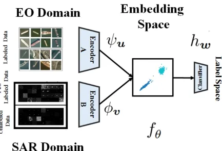
Figure1presents a block diagram visualization of our framework. In the figure, we have visualized images 237
from two related real world SAR and EO datasets that we have used in the experimental section of the paper. 238
The task is classify Ship images. Notice that SAR images are confusing for the untrained human eye, while EO 239
ship/no-ship images can be distinguished by minimal inspection. This suggests that as we discussed before, SAR 240
labeling is more challenging and requires expertise. In our approach, we consider the EO deep network fθ(·)to 241
be formed by a feature extractorφv(·), i.e. convolutional layers of the network, which is followed by a classifier
242
sub-networkhw(·), i.e. fully connected layers of the network, that inputs the extracted feature and maps them
243
to the label space. Here,wandvdenote the corresponding learnable parameters for these sub-networks, i.e. 244
θ= (w,v). This decomposition is synthetic but helps to understand our approach. In other words, the feature 245
extractor sub-networkφv :X → Zmaps the data points into a discriminative embedding spaceZ ⊂Rf, where
246
classification can be done easily by the classifier sub-networkhw :Z → Y. The success of deep learning stems
247
from optimal feature extraction which converts the data distribution into a multimodal distribution which makes 248
class separation feasible. Following the above, we can consider a second encoder networkψu(·):Rd →Rf,
249
which maps the SAR data points to the same target embedding space at its output. The idea that we want to 250
explore is based on trainingφvandψusuch that the discrepancy between the source distributionpS(φ(x))and 251
target distributionpT(φ(x))is minimized in the shared embedding space, modeled as the shared output space 252
of these two encoders. As a result of matching the two distributions, the embedding space becomes invariant 253
with respect to the domain. In other words, data points from the two domains become indistinguishable in the 254
embedding space, e.g. data points belonging to the same class are mapped into the same geometric cluster in the 255
shared embedding space as depicted in Figure1. Consequently, even if we train the classifier sub-network using 256
solely the source labeled data points, it will still generalize well when target data points are used for testing. The 257
key question is how to train the encoder sub-networks such that the embedding space becomes invariant. We 258
need to adapt the standard supervised learning in Eq. (1) by adding additional terms that enforce cross-domain 259
distribution matching. 260
4. Proposed Solution
261
Figure 1.Block diagram architecture of the proposed framework for transferring knowledge from the EO to the SAR domain.
by minimizing the discrepancy between the distributions of both domains in the embedding space. Following the above, we can formulate the following optimization problem for computing the optimal values forv,uandw:
min v,u,w
1 N
N
∑
i=1L hw(φv(xsi)),yis
+ 1
O O
∑
i=1L hw(ψu(x 0t i)),y
0t i
+λD φv(pS(XS)),ψu(pT(XT))+η k
∑
j=1D φv(pS(XS)|Cj),ψu(pT(XT0 )|Cj)
,
(3)
whereD(·,·)is a discrepancy measure between the probabilities andλandηare trade-off parameters. The first 262
two terms in Eq. (3) are standard empirical risks for classifying the EO and SAR labeled data points, respectively. 263
The third term is the cross-domain unconditional probability matching loss. We match the unconditional 264
distributions as the SAR data is mostly unlabeled. The matching loss is computed using all available data points 265
from both domains to learn the learnable parameters of encoder sub-networks and the classifier sub-network 266
is simultaneously learned using the labeled data from both domains. Finally, the last term is Eq. (3) is added 267
to enforce semantic consistency between the two domains by match the distributions class-conditionally. This 268
term is important for knowledge transfer. To clarify this point, note that the domains might be aligned such that 269
their marginal distributionsφ(pS(XS))andψ(pT(XT))have minimal discrepancy, while the distance between
270
φ(qS(·,·))andψ(qT(·,·))is not minimized. This means that the classes may not have been aligned correctly,
271
e.g. images belonging to a class in the target domain may be matched to a wrong class in the source domain or, 272
even worse, images from multiple classes in the target domain may be matched to the cluster of another class 273
of the source domain. In such cases, the classifier will not generalize well on the target domain as it has been 274
trained to be consistent with spatial arrangement of the source domain in the embedding space. This means 275
that if we merely minimize the distance betweenφ(pS(XS))andψ(pT(XT)), the shared embedding space
276
Algorithm 1FCS(L,η,λ)
1: Input:data
2:
3: DS = (XS,YS);DT = (XT, ,YT),D0T = (XT0),
4:
5: Pre-training: initialization 6:
7: θˆ0= (w0,v0) =arg minθ1/N∑ N
i=1L(fθ(xsi),yis) 8:
9: foritr=1, . . . ,ITR do
10:
11: Updateencoder parameters using:
12:
13: v, ˆˆ u=λD φv(pS(XS)),ψu(pT(XT))
14:
15: +η∑jD φv(pS(XS)|Cj),ψv(pS L(XT0 )|Cj) 16:
17: Updateentire parameters:
18:
19: v, ˆˆ u, ˆw=arg minw,v,u1/N∑iN=1L hw(φˆˆv(xsi)),ysi 20:
21: +1/O∑Oi=1L hw(ψˆˆu(x 0t i)),y
0t i
22:
23: end for
of class-matching is a known problem in domain adaptation and several approaches have been developed to 278
address this challenge [27]. In our framework, the few labeled data points in the target SAR domain can be used 279
to match the classes consistently across both domains. We use these data points to compute the fourth term in 280
Eq. (3). This term is added to match class-conditional probabilities of both domains in the embedding space, i.e. 281
φ(pS(xS)|Cj)≈ψ(pT(x|Cj), whereCjdenotes a particular class.
282
The remaining key question is selecting a proper metric to compute D(·,·) in the last two terms of 283
Eq1. KL-divergence and Jensen-Shannon divergence have been used extensively to measure closeness of 284
probability distributions as maximizing the log-likelihood is equivalent to minimizing the KL-divergence between 285
two distributions but as we discussed since stochastic gradient descend is the standard technique to solve the 286
optimization problem in Eq1, KL-divergence and Jensen-Shannon divergence are not suitable for deep learning 287
applications. This is a major reason for success of adversarial learning as the discrepancy beteen two distributions 288
is minimized indirectly without requiring minimizing a metric [21]. Additionally, the distributionsφ(pS(x)and
289
ψ(pT(x)are unknown and we can rely only on observed samples from these distributions. Therefore, we should
290
be able to compute the discrepancy measure,D(·,·)using only the drawn samples. Optimal transport [16] is a 291
suitable metric to deal with the above issues. For this reason, it has been found to be an effective metric and has 292
been used extensively in deep learning literature recently [15,22,28,29]. Wasserstein Distance is defined in terms 293
of an optimization problem which can be computationally expensive to solve for high-dimensional data. For this 294
reason, efficient approximations and variants for it has been an active research area. In this paper, we use the 295
Sliced Wasserstein Distance (SWD) [30] which is a good approximate of optimal transport [19] and additionally 296
can be computed more efficiently. 297
Although the Wasserstein distance is defined as the solution to a linear programming problem, but for the case of one-dimensional probability distributions, this problem has a closed form solution which can be computed efficiently. The solution is equal to the`p-distance between the inverse of the cumulative distribution functions of the two distributions. SWD has been proposed to benefit from this property to simplify computation of the Wasserstein distance. The idea is to decompose ad-dimensional distributions into one-dimension marginal distributions by projecting the distribution along all possible hyperplanes that cover the space. This process is called slicing the high-dimensional distributions. For a distributionpS, a one-dimensional slice of the distribution
along the projection directionγis defined as:
RpS(t;γ) = Z
SpS(x)δ(t− hγ,xi)dx , (4)
where δ(·) denotes the Kronecker delta function, h·,·i denotes the vector dot product, and Sd−1 is the 298
d-dimensional unit sphere. We can see thatRpS(·;γ)is computed via integratingpS over the hyperplanes
299
The SWD is computed by integrating the Wasserstein distance between sliced distributions over allγ: 301
SW(pS,pT) = Z
Sd−1
W(RpS(·;γ),RpT(·;γ))dγ , (5)
whereW(·,·)denotes the Wasserstein distance. Computing the above integral directly, is computationally 302
expensive. But, we can approximate the integral in Eq. (5) using a Monte Carlo style integration by choosing 303
L number of random projection directions γ and after computing the Wasserstein distance, average along 304
the random directions. Doing so, our approximation is proportional toO(√1
L)and hence we can get a good 305
approximation using Monte Carlo approximation. 306
In our problem, since we have access only to samples from the two source and target distributions, so we approximate the one-dimensional Wasserstein distance as the `p-distance between the sorted samples, as the empirical commutative probability distributions. Following the above procedure, the SWD between f-dimensional samples{φ(xSi ) ∈ Rf ∼ pS}Mi=1and{φ(xTi ) ∈ Rf ∼ pT}Mj=1can be approximated as the
following sum:
SW2(pS,pT)≈ 1
L
L
∑
l=1
M
∑
i=1
|hγl,φ(xSs
l[i]i)− hγl,φ(x T
tl[i])i|
2 , (6)
whereγl ∈Sf−1is uniformly drawn random sample from the unit f-dimensional ballSf−1, andsl[i]andtl[i] 307
are the sorted indices of{γl·φ(xi)}iM=1for source and target domains, respectively. We utilize the SWD as the 308
discrepancy measure between the probability distributions to match them in the embedding space. Our proposed 309
algorithm for few-shot SAR image classification (FSC) using cross-domain knowledge transfer is summarized in 310
Algorithm1. Note that we have added a pretraining step which trains the EO encoder and the shared classifier 311
sub-network solely on the EO domain, to be used a better initial point for the next steps of the optimization. 312
Since our problem is non-convex, a good initial point is critical for finding a good local solution. 313
5. Theoretical Analysis
314
In order to demonstrate that our approach is effective, we show that transferring knowledge from the EO 315
domain can reduce the real task on the SAR domain. Our analysis is based on broad results for domain adaptation 316
and is not limited to the case of EO-to-SAR transfer. We rely on theoretical results that demonstrate the true target 317
risk for a model that is trained on a source domain is upperbounded by the discrepancy between distributions of 318
the source and the target domains. Various works have used different discrepancy measures for this analysis, but 319
we rely on a version for which optimal transport is used as the discrepancy measure [15]. We use this result and 320
demonstrate why training procedure of our algorithm can train models that generalize well on the target domain. 321
Redko et al. [15] analyze a standard domain adaptation framework, where the same shared classifierhw(·) is used on both the source and the target domain. This is analogous to our formulation as the classifier network is shared across the domains in our framework. They use a standard PAC-learning formalism. Accordingly, the hypothesis class is the set of all modelhw(·)that are parameterized byθand the goal is to select the best model from the hypothesis class. For any member of this hypothesis class, we denote the true risk on the source domain byeS and the true risk on the target domain witheT. Analogously,µˆS = N1 ∑Nn=1δ(xsn)denote the empirical marginal source distribution, which is computed using the training samples andµˆT = M1 ∑mM=1δ(xtm) similarly denotes the empirical target distribution. In this setting, conditioned on availability of labeled data on both domains, we can train a model jointly on both distributions. Lethw∗ denote such a ideal model that minimizes the combined source and target riskseC(w∗):
w∗=arg min
w eC(w) =arg minw {eS+eT} . (7)
If the hypothesis class is complex enough and given sufficient labeled target domain data, the joint model can be 322
trained such that it generalizes well on both domains. This term is to measure an upperbound for the target risk. 323
Redko et al. [22] proved the following theorem in standard domain adaptation which provides an upper-bound on 324
Theorem 5.1. [15] Under the assumptions described above for UDA, then for anyd0>dandζ< √
2, there exists a constant numberN0depending ond0such that for anyξ>0andmin(N,M)≥max(ξ−(d
0+2),1 )with probability at least1−ξfor allhw, the following holds:
eT ≤eS+W(µˆT, ˆµS) +eC(w∗) +
s
2 log(1 ξ)/ζ
r
1
N+
r
1 M
. (8)
Note that although we use SWD in our approach, but it has been theoretically demonstrated that SWD is a good 326
approximation for computing the Wasserstein distance [31]: 327
SW2(pX,pY)≤W2(pX,pY)≤αSW2β(pX,pY) (9)
whereαis a constant andβ= (2(d+1))−1(see [32] for more details). For this reasons, minimizing the SWD 328
metric enforces minimizing WD. 329
The proof for Theorem5.1is based on the fact that the Wasserstein distance between a distributionµand its empirical approximationµˆusingNidentically drawn samples can be be made small as desired given existence of large enough number of samplesN[15]. More specifically, in the setting of Theorem5.1, we have:
W(µ, ˆµ)≤ s
2 log(1 ξ)/ζ
r
1
N . (10)
We need this property for our analysis. Additionally, we consider bounded loss functions and consider the 330
loss function is normalized by its upperbound. Interested reader may refer to Redko et al. for more details of 331
derivation of this property [15]. 332
Inspection of the Theorem5.1might lead to the conclusion that if we minimize the Wasserstein distance 333
between the source and the target marginal distributions in the input space of the model, then we can improve 334
generalization error on the target domain as doing so the upperbound on the target true risk will become tighter 335
in Eq. (8). Thus, performance on the target domain will be close to the performance on the source domain which 336
is small for a model with good performance on the source domain. But there is no guarantee that if we solely 337
minimize the distance between the marginal distributions, then a joint optimal modelhw∗with small joint error 338
would exist. This is important as the third term in the right hand side of Eq. (8) would become small only if such 339
a joint model exists. This conclusion might seem unintuitive, but consider a binary classification problem. This 340
situation can happen if the wrong classes are matched across the two domains. In other words, we may minimize 341
the distance between the marginal distribution, but data points from each class are matched to the opposite class 342
in the other domain. Then training a joint model that performs well for both classes is not possible. Hence, we 343
need to minimize the Wasserstein distance between the marginal distributions such that analogous classes across 344
the domains align in the embedding space in order to consider all terms in Theorem5.1. In our algorithm, the 345
few target labeled data points are used to minimize the joint order. Building upon the above result, we provide 346
the following lemma for our algorithm. 347
Lemma 5.1. Consider we use the target dataset labeled data in a semi-supervised domain adaptation scenario
in the algorithm1. Then, the following inequality for the target true risk holds:
eT ≤eS+W(µˆS, ˆµP L) +eˆC0(w∗) +
s
2 log(1 ξ)/ζ
2
r
1
N+
r
1
M+
r
1 O
, (11)
whereeˆC0(w∗)denote the empirical risk of the optimally joint modelhw∗on both the source domain and the 348
target labeled data points. 349
Proof:We useµTSto denote the combined distribution of both domains. The model parameterw∗is trained 350
for this distribution using ERM on the joint empirical distribution:µˆTS= N1 ∑Nn=1δ(xsn) +O1∑ O n=1δ(x
note that given this definition and considering the corresponding joint empirical distribution,pST(x,y), it is easy 352
to show thateTSˆ =eˆC0(w∗). In other words, we can denote the empirical risk for the model as the true risk for
353
the empirical distribution. 354
eC0(w∗) =eˆC0(w∗) + eC0(w∗)−eˆC0(w∗)≤eˆC0(w∗) +W(µTS, ˆµTS)
≤eˆC0(w∗)) +
s
2 log(1 ξ)/ζ
r
1
N+
r
1 O
.
(12)
We have used the definition of expectation and the Cauchy-Schwarz inequality to deduce the first inequality in 355
Eq. (12). We have also used the above mentioned property of the Wasserstein distance in Eq. (10) to deduce the 356
second inequality. Now combining Eq. (12) and Eq. (8) completes our proof. 357
According to Lemma5.1, the most important samples are the few labeled samples in the target domain as 358
the corresponding term is dominant among the constant terms in Eq. (11) (noteOMandON). As we 359
argued, these samples are important to circumvent the class matching challence across the two domains. 360
6. Experimental Validation
361
In section we validate our approach empirically. We demonstrated effectiveness of our method in the area 362
of maritime domain awareness on SAR ship detection problem. 363
6.1. Ship detection in SAR domain 364
We tested our approach in the binary problem of ship detection using SAR imaging [6]. This problem arises 365
within maritime domain awareness (MDA) where the goal is monitoring ocean continually to decipher maritime 366
activities that could impact the safety of the environment. Detecting ships is important in this application as the 367
majority of important activities that are important is related to ships and their movements. Traditionally, planes 368
and patrol vessels are used for monitoring, but these methods are effective only for limited areas and time periods. 369
As the regulated area expands and monitoring period becomes extended, these methods become time consuming 370
and inefficient. To circumvent these limitations, it is essential to make this process automatic such that it requires 371
minimal human intervention. To reach this goal, satellite imaging is highly effective because large areas of ocean 372
can be monitored. The generated satellite images can be processed using image processing and machine learning 373
techniques automatically. Satellite imaging has been performed using satellite with both EO and SAR imaging 374
devices. However, only SAR imaging allows continual monitoring during broad range of weather conditions 375
and during night. This property is important because illegal activities likely to happen during night and during 376
occluded weather, human errors are likely to occur. For these reasons, SAR imaging is very important in this 377
area and hence we can test our approach on this problem. 378
When satellite imaging is used, we a huge amount of data is generated. But, a large portion of data is 379
not informative because the huge portion of images contain only surface of ocean with no important object of 380
interest or potentially land areas adjacent to sea. In order to make the monitoring process efficient, classic image 381
processing techniques are used to determine regions of interest in aerial SAR images. A region of interest is a 382
limited surface area, where existence of a ship is probable. First, land areas are removed and then ships, ship-like, 383
and ocean regions are identified and then extracted as square image patches. These image patches are then fed 384
into a classification algorithm to determine whether the region corresponds to a ship or not. If a ship detected 385
with suspicious movement activity, then regulations can be enforced. 386
The dataset that we have used in our experiments is obtained from aerial SAR images of the South African 387
Exclusive Economic Zone. The dataset is preprocessed into51×51pixels sub-images [6]. We define a binary 388
classification problem, where each image instance is either contains ships (positive data points), or no-ship 389
(negative data points). The dataset contains 1436 positive examples and 1436 negative sub-images. The labels 390
are provided by experts. We recast the problem as a few-shot learning problem by assuming that only few of the 391
data points are labeled. To solve this problem using knowledge transfer within our framework, we use the “EO 392
supply chain analysis and contains EO images extracted from Planet satellite imagery over the San Francisco 394
Bay area with 4000 RGB80×80images. Again, each instance is either a ship image (a positive data point), or 395
no-ship (a negative data point). The dataset is split evenly into positive and negative samples. Instances from 396
both datasets are visualized in Figure1(left). 397
6.2. Methodology 398
We consider a deep CNNs with 2 layers of convolutional3×3filters as SAR encoder. We useNFand2NF 399
filters in these layers respectively, whereNFis parameter to be determined. We have used both maxpool and 400
batch normalization layers in these convolutional layers. These layers are used as the SAR encoder sub-network 401
in our framework,φ. We have used a similar structure for EO domain encoder,ψ, with the exception of using 402
a CNN with three convolutional layers. The reason is that the EO dataset seems to have more details and 403
more complex model can learn information content better. The third convolutional layer has2NF filters as 404
well. The convolutional layers are followed by a flattening layer and a subsequent shared dense layer as the 405
embedding space with dimension f which can be tuned as a parameter. After the embedding space layer, we have 406
used a shallow two-layer classifier based on Eq. (3). We used TensorFlow for implementation and the Adam 407
optimizer [34]. 408
For comparison purpose, we compared our results against the following learning settings: 409
1) Supervised training on the SAR domain (ST): we just trained a network directly in the SAR domain using 410
the few labeled SAR data points to generate a lower-bound for approach to demonstrate that knowledge transfer is 411
effective. This approach is also a lower-bound because unlabeled SAR data points and their information content 412
are discarded. 413
2) Direct transfer (DT): we just directly used the network that is trained on EO data directly in the SAR 414
domain. In order to do this end, we resized the EO domain to51×51pixels so we can use the same shared 415
encoder networks for both domains. As a result, potentially helpful details may be lost. This can be served as a 416
second lower-bound to demonstrate that we can benefit from unlabeled SAR data. 417
3) Fine tuning (FT): we used the no transfer network from previous method, and fine-tuned the network 418
using the few available SAR data points. As discussed before in the “Related Work" section, this is the main 419
strategy that several prior works have used in the literature to transfer knowledge from the EO to the SAR domain 420
and is served to compare against previous methods that use knowledge transfer. 421
In our experiments, we used a 90/10 % random split for training the model and testing performance. For 422
each experiment, we report the performance on the SAR testing split to compare the methods. We use the 423
classification accuracy rate to measure performance and whenever necessary and we used cross validation to 424
tune the hyper parameters. We have repeated each experiment 20 times and have reported the average and the 425
standard error bound to demonstrate statistical significance in the experiments. 426
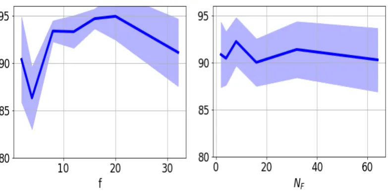
In order to find the optimal parameters for the network structure, we used cross validation. We first 427
preformed a set of experiments to empirically study the effect of dimension size (f) of the embedding space 428
on performance of our algorithm. Figure2a presents performance on SAR testing set versus dimension of 429
the embedding space when 10 SAR labeled data per class is used for training. The solid line denotes the 430
average performance over ten trials and the shaded region denotes the standard error deviation. We observe 431
that the performance is quite stable when the embedding space dimension changes. This result suggests that 432
because convolutional layers are served to reduce the dimension of input data, if the learned embedding space is 433
discriminative for the source domain, then our method can successfully match the target domain distribution to 434
the source distribution in the embedding. We conclude that for computational efficiency, it is better to select the 435
embedding dimension to be as small as possible. We conclude from Figure2athat increasing the dimension 436
beyond 8 is not helpful. For this reason, we set the dimension of the embedding to be 8 for the rest our experiments 437
in this paper. We performed a similar experiment to investigate the effect of number of filtersNFon performance. 438
Figure2bpresents performance on SAR testing set versus this parameter. We conclude from Figure2bthat 439
NF =16is a good choice as using more filters in not helpful. We did not used a less value forNF to avoid 440
(a)Performance vs Embedding Dimension (b)Performance vs Number of Filters Figure 2.The SAR test performance versus the dimension of the embedding space and the number of filters.
O 1 2 3 4 5 6 7
ST 58.5 74.0 79.2 84.1 85.2 84.9 87.2 FT 75.5 75.6 73.5 85.5 87.6 84.2 88.5 DT 71.5 67.6 71.4 68.5 71.4 71.0 73.1 FCS 86.3 86.3 82.8 94.2 87.8 96.0 91.1 Table 1.Comparison results for the SAR test performance.
6.3. Results 442
Figure3presents the performance results on the data test split for our method along with the three mentioned 443
methods above, versus the number of labeled data points per class that has been used for the SAR domain. For 444
each curve, the solid line denotes the average performance over all ten trials and the shaded region denotes 445
the standard error deviation. These results accord with intuition. It can be seen that direct transfer is the least 446
effective method as it uses no information from the second domain. Supervised training on the SAR domain is 447
not effective in few shot learning regime, i.e. its performance is close to chance. Direct transfer method boosts 448
the performance of supervised training in one-shot regime but after 2-3 labeled samples per class, as expected 449
supervised training overtakes direct transfer. This is the consequence of using more target task data. In other 450
words, direct transfer only helps to test the network on a better initial point compared to random initialization. 451
Fine tuning can improve the direct performance, but only few-shot regime, and beyond few-shot learning regime 452
the performance is similar to supervised training. In comparison, our method outperforms these methods as we 453
have benefited from SAR unlabeled data points. For a more clear quantitative comparison, we have presented 454
data in Figure3in Table1for different number of labeled SAR data points per class (O). It is also important to 455
note that in the presence of enough labeled data in the target domain, supervised training would outperform our 456
method because the netowkr is trained using solely the target domain data. 457
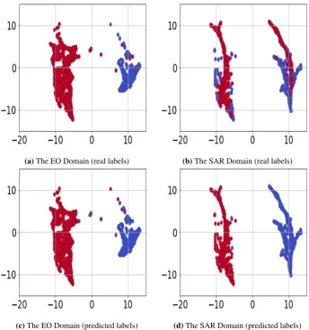
For having better intuition, Figure4denotes the Umap visualization [35] of the EO and SAR data points in 458
the learned embedding as the output of the feature extractor encoders. Each points denotes on data point in the 459
embedding which has been mapped to 2D plane for visualization. In this figure, we have used 5 labeled data 460
points per class in the SAR domain. In Figure4, each color corresponds to one of the classes. In Figures4a
461
and 4b, we have used real labels for visualization, and in Figures4cand 4d, we have used the predicted labels 462
by networks trained using our method for visualization. In Figure4, the points with brighter red and darker 463
blue colors are the SAR labeled data points that has been used in training. By comparing the top row with the 464
bottom row, we see that the embedding is discriminative for both domains. Additionally, by comparing the 465
Figure 3.The SAR test performance versus the number of labeled data per class.
(a)The EO Domain (real labels) (b)The SAR Domain (real labels)
(c)The EO Domain (predicted labels) (d)The SAR Domain (labeled and unlabeled data) Figure 4.Umap visualization of the EO versus the SAR dataset in the shared embedding space. (view in color.)
conditionally, suggesting our framework formulated is Eq. (3) is effective. This result suggests that learning an 467
invariant embedding space can be served as a helpful strategy for transferring knowledge. Additionally, we see 468
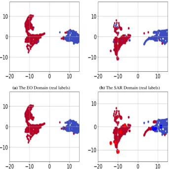
(a)The EO Domain (real labels) (b)The SAR Domain (real labels)
(c)The EO Domain (predicted labels) (d)The SAR Domain (predicted labels) Figure 5.Umap visualization of the EO versus the SAR dataset for ablation study. (view in color.)
part of one of the classes (blue) is predicted mistakenly. This observation suggests that the boundary between 470
classes depends on the labeled target data as the network is certain about labels of these data points. 471
We also performed an experiment to serve as an ablation study for our framework. Our previous experiments 472
demonstrate that the first three terms in Eq. (3) are all important for successful knowledge transfer. We explained 473
that the fourth term is important for class-conditional alignment. We solved Eq. (3) without considering the 474
fourth term to study its effect. We have presented the Umap visualization of the datasets in the embedding 475
space for a particular experiment in Figure5. We observe that as expected the embedding is discriminative for 476
EO dataset and predicted labels are close to the real data labels as the classes are separable. However, despite 477
following a similar marginal distribution in the embedding space, the formed SAR clusters are not class-specific. 478
We can see that in each cluster, we have data points from both classes and as a result the SAR classification rate 479
is poor. This result demonstrates that all the terms in Eq. (3) are important for the success of our algorithm. We 480
highlight that Figure5visualizes results of a particular experiments and we observed in some experiments the 481
classes were matched, even when no labeled target data was used. However, this observations shows that the 482
method is not stable. Using the few-labeled data helps to stabilize the algorithm. 483
7. Conclusions
484
In this paper, we addressed the problem of SAR image classification when only few labeled data are 485
available. We formulated this problem as a semi-supervised domain adaption problem. Our idea is based on 486
transferring knowledge from a related electro-optical domain problem where it is easy to generate labeled data. 487
The networks are trained such that the convolutional layers are served as two deep encoders that match the 489
distributions of the two EO and SAR domains in an embedding space which is modeled as their shared output 490
space. We provided theoretical analysis to explain why our algorithm minimizes an upperbound for target real 491
risk and demonstrated effectiveness and applicability of our approach for the problem of ship classification in the 492
area of maritime domain awareness. Despite being effective, a major restriction of our method is full overlap 493
between the existing classes across the EO and the SAR domain. A future research direction is to remove this 494
restriction by training the networks such that only the shared classes are matched in the embedding space. 495
496
1. Koo, V.; Chan, Y.; Vetharatnam, G.; Chua, M.Y.; Lim, C.; Lim, C.; Thum, C.; Lim, T.; bin Ahmad, Z.; Mahmood, 497
K.; others. A new unmanned aerial vehicle synthetic aperture radar for environmental monitoring. Progress In 498
Electromagnetics Research2012,122, 245–268. 499
2. Maitre, H.Processing of Synthetic Aperture Radar (SAR) Images; Wiley, 2010. 500
3. Deng, J.; Dong, W.; Socher, R.; Li, L.J.; Li, K.; Fei-Fei, L. Imagenet: A large-scale hierarchical image database. 501
2009 IEEE conference on computer vision and pattern recognition. Ieee, 2009, pp. 248–255. 502
4. Rostami, M.; Huber, D.; Lu, T.C. A crowdsourcing triage algorithm for geopolitical event forecasting. Proceedings 503
of the 12th ACM Conference on Recommender Systems. ACM, 2018, pp. 377–381. 504
5. Malmgren-Hansen, D.; Kusk, A.; Dall, J.; Nielsen, A.; Engholm, R.; Skriver, H. Improving SAR automatic target 505
recognition models with transfer learning from simulated data. IEEE Geoscience and Remote Sensing Letters2017, 506
14, 1484–1488. 507
6. Schwegmann, C.; Kleynhans, W.; Salmon, B.; Mdakane, L.; Meyer, R. Very deep learning for ship discrimination in 508
synthetic aperture radar imagery. IEEE International Geo. and Remote Sensing Symposium, 2016, pp. 104–107. 509
7. Huang, Z.; Pan, Z.; Lei, B. Transfer learning with deep convolutional neural network for SAR target classification 510
with limited labeled data.Remote Sensing2017,9, 907. 511
8. Chen, S.; Wang, H.; Xu, F.; Jin, Y. Target classification using the deep convolutional networks for SAR images. IEEE 512
Trans. on Geo. and Remote Sens.2016,54, 4806–4817. 513
9. Shang, R.; Wang, J.; Jiao, L.; Stolkin, R.; Hou, B.; Li, Y. SAR Targets Classification Based on Deep Memory 514
Convolution Neural Networks and Transfer Parameters. IEEE Journal of Selected Topics in Applied Earth 515
Observations and Remote Sensing2018,11, 2834–2846. 516
10. Pan, S.; Yang, Q. A survey on transfer learning. IEEE Transactions on knowledge and data engineering2010, 517
22, 1345–1359. 518
11. Zhang, D., J.; Heng, W.; Ren, K.; Song, J. Transfer Learning with Convolutional Neural Networks for SAR Ship 519
Recognition. IOP Conference Series: Materials Science and Engineering. IOP Publishing, 2018, Vol. 322, p. 072001. 520
12. Wang, Z.; Du, L.; Mao, J.; Liu, B.; Yang, D. SAR Target Detection Based on SSD With Data Augmentation and 521
Transfer Learning. IEEE Geoscience and Remote Sensing Letters2018. 522
13. Lang, H.; Wu, S.; Xu, Y. Ship classification in SAR images improved by AIS knowledge transfer.IEEE Geoscience 523
and Remote Sensing Letters2018,15, 439–443. 524
14. Motiian, S.; Jones, Q.; Iranmanesh, S.; Doretto, G. Few-shot adversarial domain adaptation. Advances in Neural 525
Information Processing Systems, 2017, pp. 6670–6680. 526
15. Redko, I.and Habrard, A.; Sebban, M. Theoretical analysis of domain adaptation with optimal transport. Joint 527
European Conference on Machine Learning and Knowledge Discovery in Databases. Springer, 2017, pp. 737–753. 528
16. Villani, C.Optimal transport: old and new; Vol. 338, Springer Science & Business Media, 2008. 529
17. Gretton, A.; Smola, A.; Huang, J.; Schmittfull, M.; Borgwardt, K.; Schölkopf, B. Covariate shift by kernel mean 530
matching. Dataset shift in machine learning2009. 531
18. Rabin, J.; Peyré, G.; Delon, J.; Bernot, M. Wasserstein barycenter and its application to texture mixing. International 532
Conference on Scale Space and Variational Methods in Computer Vision. Springer, 2011, pp. 435–446. 533
19. Kolouri, S.; Rohde, G.K.; Hoffman, H. Sliced Wasserstein Distance for Learning Gaussian Mixture Models. IEEE 534
Conference on Computer Vision and Pattern Recognition, 2018, pp. 3427–. 535
20. Kodirov, E.; Xiang, T.; Fu, Z.; Gong, S. Unsupervised domain adaptation for zero-shot learning. Proceedings of the 536
IEEE International Conference on Computer Vision, 2015, pp. 2452–2460. 537
21. Goodfellow, I.; Pouget-Abadie, J.; Mirza, M.; Xu, B.; Warde-Farley, D.; Ozair, S.; Courville, A.; Bengio, Y. 538
22. Courty, N.; Flamary, R.; Tuia, D.; Rakotomamonjy, A. Optimal transport for domain adaptation. IEEE TPAMI2017, 540
39, 1853–1865. 541
23. Daume III, H.; Marcu, D. Domain adaptation for statistical classifiers. Journal of artificial Intelligence research 542
2006,26, 101–126. 543
24. Kolouri, S.; Pope, P.E.; Martin, C.E.; Rohde, G.K. Sliced-Wasserstein Auto-Encoders. International Conference on 544
Learning Representation (ICLR)2019. 545
25. Bonneel, N.; Rabin, J.; Peyré, G.; Pfister, H. Sliced and Radon Wasserstein barycenters of measures. Journal of 546
Mathematical Imaging and Vision2015,51, 22–45. 547
26. Carriere, M.; Cuturi, M.; Oudot, S. Sliced wasserstein kernel for persistence diagrams. arXiv preprint 548
arXiv:1706.033582017. 549
27. Long, M.; Wang, J.; Ding, G.; Sun, J.; Yu, P.S. Transfer joint matching for unsupervised domain adaptation. 550
Proceedings of the IEEE conference on computer vision and pattern recognition, 2014, pp. 1410–1417. 551
28. Damodaran, B.; Kellenberger, B.; Flamary, R.; Tuia, D.; Courty, N. DeepJDOT: Deep Joint distribution optimal 552
transport for unsupervised domain adaptation.arXiv preprint arXiv:1803.100812018. 553
29. Kolouri, S.; Park, S.R.; Thorpe, M.; Slepcev, D.; Rohde, G.K. Optimal Mass Transport: Signal processing and 554
machine-learning applications. IEEE Signal Processing Magazine2017,34, 43–59. 555
30. Rabin, J.; Peyré, G.; Delon, J.; Bernot, M. Wasserstein barycenter and its application to texture mixing. International 556
Conference on Scale Space and Variational Methods in Computer Vision. Springer, 2011, pp. 435–446. 557
31. Bonnotte, N. Unidimensional and evolution methods for optimal transportation. PhD thesis, Paris 11, 2013. 558
32. Santambrogio, F. Optimal transport for applied mathematicians. Birkäuser, NY2015, pp. 99–102. 559
33. Hammell, R. Ships in Satellite Imagery, 2017. data retrieved from Kaggle, https://www.kaggle.com/rhammell/ships-560
in-satellite-imagery. 561
34. Kingma, D.P.; Ba, J. Adam: A method for stochastic optimization. arXiv preprint arXiv:1412.69802014. 562
35. McInnes, L.; Healy, J.; Melville, J. Umap: Uniform manifold approximation and projection for dimension reduction. 563