An Enhanced Distributed Data Aggregation Method in the Internet of Things

An Enhanced distributed data aggregation

method in the internet of things

M.H, Homaei, Ely Salwana, Shahab Shamshirband

1Internet of Things Laboratory of Iran (Gloriot), Iran.

2Institute of Visual Informatics, Universiti Kebangsaan Malaysia

3 Department for Management of Science and Technology Development, Ton Duc Thang University, Ho Chi Minh City, Viet Nam 4 Faculty of Information Technology, Ton Duc Thang University, Ho Chi Minh City, Viet Nam

• E-mail: [email protected]

Abstract—As a novel concept in technology and communication world, “Internet of Things (IoT)” has been emerged. In such modern technology, the capability to transmit data through data communication networks (such as Internet or Intranet) is provided for each organism (e.g. human being, animals, things, and so forth). Due to the limited hardware and communication operational capability as well as small dimensions, IoT undergoes quite a few challenges. Such inherent challenges not only cause fundamental restrictions in the efficiency of aggregation, transmission, and communication between nodes; but they also degrade routing performance. To cope with the reduced availability time and unstable communications among nodes, data aggregation and transmission approaches in such networks are designed more intelligently. In this paper, a distributed method is proposed to set child balance among nodes. In this method, the height of the network graph is increased through restricting the degree; and network congestion is reduced as a result. Besides, a dynamic data aggregation approach -named as LA-RPL- is proposed for RPL networks. More specifically, each node is equipped with learning automata in order to perform data aggregation and transmissions. Simulation results demonstrate that the proposed approach outperforms previously suggested based approaches in terms of energy consumption, network control overhead, and packet loss rate.

Index Terms—Data aggregation methods, Learning automata, RPL, Routing, Internet of Thing (IoT).

—————————— ◆ ——————————

1 I

HE expression “every Internet-connected thing is alive” will be a new rule in the near future. Future networks are merely IoT, toward which all researches will soon be converged. Similar to the procedure of using Internet by hu-mans; from now on, new devices will be the main users of Internet ecosystem. The attention of recent researchers have been devoted to newly emerged technologies for manufacturing scalable IoT. However, the speed of comprehending the IoT framework has been decremented due to a number of factors, among which the combination of different devices, secure connections, trust management, and the collaboration between devices and systems are highlighted. Such devices collaborate in order to aggregate, share, and conduct information in a multi-hop manner. The bulk of information con-tinuously generated by IoT necessitates the conversion of aggregated data into intelligence. Such an intelligent environ-ment can play a vital role in data routing of networks [1], [2]. The consistent mobility of most of IoT nodes leads to the alternative communication between devices, and variable network topology as a result. Due to such frequent topology variations as well as the limited resources existing in today’s IoT devices, routing scheme of such networks is currently regarded as a significant challenge in the research world [3].

Coverage, sensing, connection and communication of each node in IoT requires the expenditure of energy and cost. As IoT equipments are becoming more and more portable and smaller, the energy limitation of such equipments is a con-sequential and challenging issue to be addressed [4]. Thus, prolonging the lifetime of network nodes in order to provide longterm monitoring is considered as one of the staple goals of myriads of IoT protocols. On the other hand, as the rate of the generated and transmitted data toward the base station of network is remarkably significant, the data aggregation procedure in IoT nodes is also costly. The basic goal of data aggregation methods is to collect and classify data packets in an acceptably efficient manner in terms of energy consumption rate, network lifetime, traffic bottleneck, and data purity. The type and approach of the employed data aggregation method varies based on the topology type, communi-cation type, network design, and data generation rate. In data aggregation procedure, if the median nodes do not per-form accurately, the base station will not be able to provide an accurate estimation of the received data; all of which result in the efficiency decline of the network. Hence, data aggregation approaches play a momentous role in monitoring purposes as well as the long-term observation of environment[5]. In this paper, an efficient distributed data aggregation method for IoT is proposed. Not with standing dozens of common approaches, calculation overhead of the proposed method is negligible. Moreover, as the network traffic varies, the proposed method still makes correct decisions auto-matically. The rest of this paper is organized as follows. System model and related works regarding IoT and data aggre-gation methods are presented in Sec.II. In Sec.III, a novel distributed data aggreaggre-gation method is proposed. Performance

T

evaluation of the proposed method in simulation and practical environments are respectively illustrated in Sec.IV and V. Finally, Sec.VI concludes the paper.

2 SYSTEM

MODEL

AND

RELATED

WORKS

2.1 Internet of Things architecture

Since IoT is to connect a considerable number of heteroge- nous things through Internet, this technology is significantly dependant on the existance of a flexible layer architecture. In other words, IoT is to bridge the real world and virtual world such that dynamic communication is ensured[6]. Therefore, IoT requires a novel architecture in order to obviate the inherent challenges as well as providing acceptable scalability and Quality of Service (QoS) in desperate applications. According to the presented architectures in [7] and [8], [9], layers of IoT are illustrated in Fig.1

• Perception layer: This layer is generally known as physical or hardware layer, and is particularly allocated to sensors and edge recognizers of network. In other words, physical and environmental parameters are converted into sensed data in this layer. The output of this layer will be considered as the input of network layer.

• Network layer: The main goal of this layer is to provide both direct and indirect communications between all things and IoT equipment, such that all of them are capable to send and receive data in the network. Note that the communicative infrastructures managed by network layer include all wireless communication technologies. • Middleware layer: The main task of this layer is to combine names and addresses in order to serve other

compo-nents of the network. Programmers of IoT are endeavoring to connect heterogenous things under a communica-tive platform, such that a united concept of network is created and exchanged data in databases can be saved and restored.

• Application layer: This layer usually merges and evaluates the services provided by other layers. This layer can present high-quality services for responding to the final user’s applications.

• Business layer: Also known as the management layer of all components of IoT network, is to analyze and sche-matize data.

Fig. 1. IoT architecture [10]

2.2 Data aggregation strategies in IoT

Fig. 2. Data aggregation architecture [13].

1) Cluster-based mechanisms: In cluster-based mechanisms, the network environment is divided into different clusters while each cluster comprises a number of sensor nodes [14]. In each cluster, one node is selected as the head of all other nodes in a cluster. This will not only decrease the number of transmitted packets, but it also reduces the transmission overhead and bandwidth consumption in transmissions from the cluster to a base station. In[15], a data storage system is presented, which has an efficient functionality in terms of security, scalability, flexibility, and reliability in IoT to be used in the procedure of enormous data analysis. The proposed approach of this research is to present a distributed storage infrastructure providing scalability and reliability in IoT. Multiple data storage in the distributed system pro-vides networks with fault tolerance, reliability, and stability. The general structure of cluster-based mechanisms is de-picted in Fig.3.

Fig. 3. Cluster-based architecture [7].

2) Centralized mechanisms: Another suggested data aggregation method in IoT is termed as the centralized method [16]. In this method, the data existing in all other network nodes along a route is transmitted to only one node. In other words, all nodes deliver their sensed information to a single node, which is superior to other network nodes in terms of hardware features and resources. In this method, the central node generally aggregates several data packets and converts them into a single packet [17]. In[18], an IoT communication platform is proposed, in order to support wireless sensor network nodes activity and proper data delivery rate. In this approach, while the unity of data is conserved, confidenti-ality and accessibility of the network are taken into consideration as well. However, the complexity of this data aggre-gation mechanism is not evaluated in practical applications. Authors in [19] presented a distributed service-driven ar-chitecture to gather data from multiple nodes in various applications of IoT. This mechanism not only alleviates network traffic, but it can also be employed as a flexible mechanism to share data in disparate programs. However, the main challenge of this mechanism is the low accessibility of the central node in the network. In addition, data will be lost if breaks occur in the central node [20].

3) Tree-based mechanisms: Another structure of IoT topology is based on trees. In this structure, tree construction is

One of the main goals of the tree-based structure in LLN networks and multi-hop wireless networks is to conserve energy as well as reducing hidden terminal effect in the network, in that by utilizing multi-hop communication, an acceptable balance is established in energy consumption rate[21], [22].

IETF group has proposed a routing scheme for low-power and lossy networks such as IoT and sensor networks, such that IPv6 protocol is extended based on RPL [23]. RPL is an extended distance vector-based protocol for IoT. Routing limitations and challenges in sensor networks, as the most salient subset of IoT, distinguishes it from all other distributed systems [24]. Such limitations affect the whole design of wireless sensor networks, including various protocols and al-gorithms of other classifications of IoT. This research has focused on the routing scheme of IoT [25]. RPL consists of an acyclic graph with one root per DODAG. In such a graph, each node acts as the parent node if required; otherwise, it is considered as a child of an accessible parent. The utilization of a point to multi-point approach is another feature of this approach, which is consistent with the applications of sensor networks. As depicted in Fig.4, this protocol creates a Destination Oriented Directed Acyclic Graph (DODAG) as the root.

Fig. 4. An illustrative network in RPL [26].

If the PAN coordinator is considered as the root of the Directed Acyclic Graph (DAG), several paths can be established toward the PAN coordinator. However, in accordance with the considered policies in RPL objective function, any kind of loop creation is avoided. RPL can exploit any routing metric to create DODAG. Each node broadcasts a DAG Infor-mation Object (DIO) containing the distance between the node and DAG root in terms of a specific metric (e.g. a number of hops, link quality, delay or Jitter). Afterwards, each node executes a distance vector algorithm, in order to find a set of neighbor nodes which are closer to the root than the node itself.

Such neighbors are the very parent nodes. Additionally, RPL presents a fast route repair mechanism to be utilized if any unstable loop is detected. Although RPL is implemented and completely evaluated in TinyOS and Contiki [4], it is rarely employed on a short MAC duty cycle. As far as the investigations of RPL reveal, RPL is not even evaluated under the operation of active beacon IEEE 802.15.4. A number of recent routing schemes support the multiple route utilization in wireless sensor networks. Authors in [27] propose the method of selecting the best path among all existing paths in order to obviate some of QoS requirements in industrial applications. To demonstrate RPL more clearly, it is crucial to define the basic principles, based on which the algorithm is proposed. In this regard, by considering an RPL network named G, consisting of node set S and boundary routers B (DODAG concept) the concepts of rank, high-priority parent of DODAG, and root list of DODAG are illustrated as follows [23]:

Definition1. Rank: Rank𝑅(𝑢, 𝑗) is a criterion of the distance between the node 𝑢 ∈ 𝑆 and DODAG root 𝑗 ∈ 𝐵. The accurate rank calculation method depends on the DAG objective function (OF). Although the rank calculation falls within the obligations of objective function, nodes’ rank should steadily decline while moving in DODAG toward DODAG destination. This is why rank can be construed as a numerical representative of the location or radius of a node within DODAG.

Definition2. DODAG Preferred Parent (DPP): Suppose node u in G, where the single-hop neighbors set is denoted by 𝑁(𝑢), and 𝐷𝑃𝑃(𝑢, 𝑗) is a limited subset of 𝑁(𝑢). For each node 𝑣 ∈ 𝑁(𝑢) we have 𝑣 ∈ 𝐷𝑃𝑃(𝑢, 𝑗), provided that v is of the minimum rank toward the specified DODAG root 𝑗 ∈ 𝐵.

Definition3. DODAG Root List (DRL): As mentioned formerly, each node 𝑣 ∈ 𝑁(𝑢) should send DIO messages in broadcast manner. In GeoRank operation, the location of DODAG root should be included in such messages. Hence, it is supposed that 𝐷𝑅𝐿(𝑗) is a saved list of DODAG root location in each node u.

Constant value k is defined such that k<|V|, where|V|is the number of existing nodes in the network graph. Constant value k, which indicates the constraint of the number of acceptable children, is recognized by each node. In other words, k is the maximum node degree in DODAG. Note that the root node does not obey this constraint. In the constitution procedure of the DODAG, each node v in DODAG selects the optimum parent p, and memorizes a potential set of alternative parents to construct upstream nodes. To implement the graph degree constraint in BD-RPL, the principle messages of RPL protocol, like DAO and DAO-ACK, are utilized.

Due to the great topological changes and the resultant requirement to synchronize and update routing tables, a great number of control messages are exchanged in most of the protocols proposed for IoT. For the aim of conserving energy in most of the equipments with limited resources, such communication costs should be controlled [29]. Authors in [22] focus on the low-power and lossy networks protocols, especially RPL, where resource limitations remarkably affect ef-ficiency. A flexible approach, named as A-RPL, is proposed in order to create and change network conditions through objective function formation framework. In this approach, network data is aggregated along with seeking the root node. The proposed data aggregation method in this protocol is so simple (maximum, minimum, average), such that depend-ing on the application of the data received by the parent node, the maximum value or minimum value is merely sent to its parent. Besides, a compatible scheduling model is proposed to optimize the number of control packets in an RPL network. In addition, a compatible MAC-based function is introduced, in order to determine the message transmission frequency based on the traffic variety and storage degree of the node.

3 PROPOSED

METHOD

In accordance with the demonstration of the previously proposed approaches in Sec 2.3, the proposed method of this paper comprises two objective functions for both network graph creation phase and aggregation-based data transmis-sion and exchange phase. In our proposed method, according to the first objective function (named as OF 1), each parent node is limited to k child nodes, where value k is determined depending on the network application type. Through the second objective function, namely OF 2, each network node is equipped with a Learning Automata. According to the status and congestion of the received packets, such a learning automata grants either data aggregation permission or instantly direct transmission permission to the parent node. Subsequent subsections are as follows. The formation of the network graph, based on the objective function OF 1, is illustrated in Sec 3.1. The proposed learning automata in the form of objective function OF 2 is presented in Sec 3.2.

3.1 Network graph formation phase

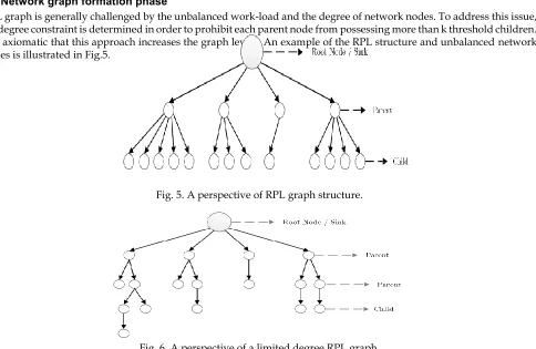
RPL graph is generally challenged by the unbalanced work-load and the degree of network nodes. To address this issue, a k degree constraint is determined in order to prohibit each parent node from possessing more than k threshold children. It is axiomatic that this approach increases the graph levels. An example of the RPL structure and unbalanced network nodes is illustrated in Fig.5.

Fig. 5. A perspective of RPL graph structure.

Fig. 6. A perspective of a limited degree RPL graph.

act of increasing network graph levels restricts the number of assigned children to a typical parent node and reduces the probability of collision and queue overflow in the network as a result.

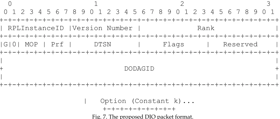
After the placement of network nodes in the environment, the root node determines the type of objective function, based on the priority of the network application type; then, the node broadcasts the degree restriction value (i.e. k constant) through DIO messages throughout the network. Note that the priority of network application type specifies the targeted end-to-end delay and packet delivery ratio. Having received the DIO message in the first level, each child node investi-gates the value of graph degree restriction (written in the Option field of DIO message) to verify whether or not this value exceeds the determined threshold. This value must not exceed the determined threshold. The proposed structure for DIO message is presented in Fig.7.

0 1 2 3

0 1 2 3 4 5 6 7 8 9 0 1 2 3 4 5 6 7 8 9 0 1 2 3 4 5 6 7 8 9 0 1

+-+-+-+-+-+-+-+-+-+-+-+-+-+-+-+-+-+-+-+-+-+-+-+-+-+-+-+-+-+-+-+-+

| RPLInstanceID |Version Number | Rank |

+-+-+-+-+-+-+-+-+-+-+-+-+-+-+-+-+-+-+-+-+-+-+-+-+-+-+-+-+-+-+-+-+

|G|0| MOP | Prf | DTSN | Flags | Reserved |

+-+-+-+-+-+-+-+-+-+-+-+-+-+-+-+-+-+-+-+-+-+-+-+-+-+-+-+-+-+-+-+-+

| |

+ DODAGID +

| |

+-+-+-+-+-+-+-+-+-+-+-+-+-+-+-+-+-+-+-+-+-+-+-+-+-+-+-+-+-+-+-+-+

| Option (Constant k)...

+-+-+-+-+-+-+-+-+

In this approach, the number of transmitted (i.e. relayed) packets in nodes placed near the sink node is not changed. However, the collision and packet loss rate decreases, which yields in the reduction of network energy consumption. According to our proposed method, in each node other than the root node, these steps are respectively followed:

1. As soon as node v selects its optimal parent (p) from DODAG, node v assists p through sending a DAO message, in order to construct the downstream routes.

2. Since p may receive DAO from different children, this node investigates the number of requests at the moment of receiving a DAO. p adopts node v as its child and adds the existing route to v into its routing table, provided that the number of accepted parental requests (including the request of node v) does not exceed k. By doing so, p informs v about acceptance of the request through sending a DAO-ACK to v. On the other hand, if the number of existing children of p exceeds k value, p denies the request of v and informs it through sending a DAO-ACK. 3. Having received the DAO-ACK message, node v creates the upstream route to p in order to stop the procedure of

DAO allocation and confirmation, provided that DAO-ACK is an accept confirmation. However, if the DAO-ACK includes a denial notification, v selects another proper parent p´ from the available parent set, and sends a DAO message to p´.

3.2 Data aggregation scheme based on learning automata

As a novel research topic, the learning mechanism of alive organisms classifies into two general categories. The first category deals with recognizing the learning principles of organisms and the relevant stages. The second category deals with presenting a methodology of placing such principles in a machine. Learning is defined as the occurred changes in a system efficiency based on the former experience. One of the consequential features of a learner systems is the ability to improve the performance of itself with the passage of time. To put in mathematical explanation, the main objective of a learner system is to optimize a task which is not completely recognized. Therefore, one of the approaches of this prob-lem is to decrease the objectives of learner system into an optimization probprob-lem defined on a set of parameters; the aim of which is to find the set of optimal parameters. A Learning Automata can be considered as an abstract object with finite number of operations. Learning Automata operates through choosing one operation from the operation set and applying that operation to the environment. The applied operation is evaluated by a random environment, and the learning au-tomata employs the environmental response to choose its next operation. During this procedure, the auau-tomata learns to choose the optimal operation. How to utilize the environmental response of the former operation in selecting the next operation is specified by the learning algorithm of the automata [30]. A learning automata consists of two main compo-nents [31]:

• A random automata with limited number of operations and a random environment communicating with the au-tomata.

Fig. 8. Stochastic Learning Automata [30].

A random automata is defined as the fourfold set 𝐿𝐴 ≡ {𝛼, 𝛽, 𝑝, 𝑇}, where 𝛼 ≡ {𝛼₁, 𝛼₂, . . . , 𝛼_𝑛} is the set of automata’s operations (n denotes the number of automata’s operation), and 𝛽 ≡ {𝛽1 , 𝛽2 , . . . , 𝛽𝑚 } is the input set of automata. The environment is denoted by the fourfold set of 𝐸 ≡ {𝛼, 𝛽, 𝑐, 𝑑}, where 𝑐 ≡ {𝑐1, 𝑐2, . . . , 𝑐𝑛} is the set of penalty probabilities and 𝑑 ≡ {𝑑₁, 𝑑₂, . . . , 𝑑_𝑛} denote the automata’s bonuses. The environment input is one of the n selected operations of the automata. The output (i.e. response) of the environment to each operation i is denoted by βi. If βi is a binary response, the environment is denominated as P-model. In such an environment, 𝛽𝑖(𝑛) = 1 is construed as the unfavorable re-sponse, or failure; and 𝛽𝑖(𝑛) = 0 is considered as favorable response, or success. Set c denoting the penalty (failure) probabilities of the environment responses is defined

𝑐_𝑖 = 𝑃𝑟𝑜𝑏{𝛽(𝑛) = 1|𝛼(𝑛) = 𝛼_𝑖}, 𝑖 = {1,2,3, … 𝑛} (1)

Where the probability of receiving an unfavorable response from the environment is denoted by 𝛼𝑖. Note that 𝛼𝑖 values are unspecified, and it is supposed that all values of 𝑐_𝑖 have a unique minimum value. In the same way, the environment can be demonstrated as a set of bonus (success) probabilities (i.e. {𝑑𝑖}) where 𝑑𝑖 denotes the probability of receiving favorable response from operation 𝛼𝑖. The relation between the random automata and environment is shown in Fig.8. This set as well as the learning algorithm are denominated as Stochastic Learning Automata. In a similar manner, the stochastic learning automata can be demonstrated by the fourfold set 𝐿𝐴 ≡ {𝛼, 𝛽, 𝑝, 𝑇}, where 𝑝 = {𝑝₁, 𝑝₂ , . . . , 𝑝_𝑛} is the border of the probabilities of automata’s operations, and 𝑇 ≡ 𝑝(𝑛 + 1) = 𝑇[𝛼(𝑛), 𝛽(𝑛), 𝑝(𝑛)] is the learning algo-rithm.

If operation 𝛼_𝑖 is selected in the 𝑛𝑡ℎ _{step; then, in the (𝑛 + 1)}𝑡ℎ _{step we have:} The favorable response from the environment is

𝑃𝑖,𝑗(𝑘 + 1) = {

𝑃𝑖,𝑗(𝑘) + 𝛼(1 − 𝑃𝑖,𝑗(𝑘)), 𝑖 = 𝑗

𝑃𝑖,𝑗(𝑘)(1 − 𝛼), ∀𝑗 ≠ 𝑖 (2) The unfavorable response from the environment is

𝑃𝑖,𝑗(𝑘 + 1) = {

𝑃𝑖,𝑗(𝑘) + (1 − 𝛽), 𝑖 = 𝑗 𝛽

𝑟−1+ 𝑃𝑖,𝑗(𝑘)(1 − 𝛽), ∀𝑗 = 𝑖 (3)

It is worth stating that set 𝛼 includes the outputs (i.e. the operations) of automata. In other words, the automata selects and applies one operation among all r operations existing in this set in each step. Note that the input set β determines the inputs of the automata [31].

Having created the network graph, network nodes execute the proposed objective function OF2. Each parent node starts either aggregating data or instantly sending data in recent time slot. The act of data aggregation is performed by each parent node such that the next-step action is selected according to the environmental received feedback. Note that the proposed system acts in distributed manner; such that if a parent node in lower layers aggregate some packets, such packets are not aggregated in higher layers, so as to avoid multi-step aggregation and the resultant unacceptable im-posed delay on data packets. In order for data aggregation mechanism to perform efficiently, each sensor node is equipped with a learning automata. Learning automata is a decision making system selecting an existing operation in the upcoming round according to the environmental received feedback. Learning automata includes two phases: select-ing phase, and learnselect-ing phase. In the selectselect-ing phase, based on the environment feedback, decisions are made with regard to the upcoming rounds toward improving the existing status in relation to previous steps [32].

1) Selecting Phase: All of the sensor nodes have an aggregation label (lbl_indicator) which is initialized to 0 at the beginning. When a sensor node plays the role as an aggregator, the value of this label changes to 1. In the routing procedure proceeding data reception, each node acts as an aggregator with probability 𝑃_𝐴𝑔𝑔 and, accordingly, acts as an ordinary node with probability 1 − 𝑃𝐴𝑔𝑔 to prepare and send the received data toward the root node. Upon the activation of lbl_indicator (i.e. changing the value to 1), the node waits for t seconds to receive more data pack-ets. Note that t is a constant value for all of the nodes acting as an aggregator. After the passage of t seconds, all the received data is aggregated into a single data packet, by means of the function F (Aggregation). Afterwards, this single packet is routed. At the beginning, all nodes have the same 𝑃_𝐴𝑔𝑔. However, through the repetitions of the algorithm and the reception of reinforcement signals from the environment, this probability changes. 2) Learning Phase: In the learning phase, a learning automata is employed in internet of things network as a

distrib-uted factor. Each node, as a learning agent, is equipped with a learning automata comprising two different oper-ations. The concepts and parameters of such a learning automata are as follows:

𝛼_(𝑛)

• Agent: Each sensor node acting as an independent learner is known as an agent. In other wards, the action of learning agent has no effect on other learning agents.

• Action: Each agent can act as an aggregator or an ordinary node.

• Reinforcement signal (S): The number of data packets received by node j during time duration t (also known as input degree).

𝑅𝑎𝑡𝑒𝑗= 𝑃𝐴𝑁 + 𝑃𝐴𝑀 (4)

Where 𝑃𝐴𝑁 is the number of data packets aggregated by previous nodes throughout the routing, and 𝑃𝐴𝑀 is the number of data packets not being aggregated by previous nodes throughout the routing.

𝑆 = 1 − 1

𝑅𝑎𝑡𝑒 𝑗 (5)

If 𝑆 > 𝑇ℎ𝑟𝑒𝑠ℎ𝑜𝑙𝑑 𝛿, then node j is rewarded. Otherwise, the node is given a penalty. If a reward is received by the node, 𝑃Agg varies as

𝑃_𝐴𝑔𝑔 = 𝑃_𝐴𝑔𝑔+ 𝛼 × 𝑅 × (1 − 𝑃_𝐴𝑔𝑔), (6) And if a bonus is received by the node, 𝑃𝐴𝑔𝑔will be as

𝑃_𝐴𝑔𝑔 = (1 − 𝛽(1 − 𝑅))𝑃_𝐴𝑔𝑔 , (7)

Where β is the penalty coefficient, T is the reward to penalty ratio, and the impact of coefficients for the total number of (plain or aggregated) received packets in node j during time duration t is

𝑁_𝐴𝑃𝑗= ∑ 𝑖 = 1𝑑𝑒𝑔𝑟𝑒𝑒 𝑁_𝑃𝐾𝑖 (8)

Where 𝑁_𝑃𝐾𝑖 is the number of aggregated data packets in i for node j, and the impact of coefficients (reward/penalty) is as

𝑇 = 1 − 1

𝑁_𝐴𝑃𝑗 (9)

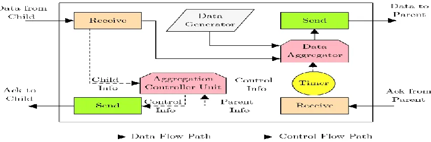
Fig. 9. The diagram of data aggregation mechanism in each parent node.

Fig. 11. General diagram of the proposed method.

The diagram of data aggregation in each parent node and data communication of nodes are respectively shown in Fig.9 and Fig.10. In addition, the general diagram of the proposed method is shown in Fig.11.

4.

PERFORMANCE

EVALUATION

In order to evaluate the performance of the proposed method and compare its performance with those of base ap-proaches Contiki Operating System and Cooja emulator are utilized. Contiki is an open source operating system for simulating IoT, which enables us to provide the communication between low power and low cost micro controllers through the Internet. Additionally, using the embedded tools in the core of Contiki Operating System, this OS provides the implementation of complex wireless networks. Contiki has been so far adapted for the hardware which is simulta-neously constrained by the memory and power, processing capability, and communication bandwidth. A Cotiki-based system usually requires resources as: a kilobyte-ranged memory capacity, a milliwatt-ranged power, a several mega-hertz-ranged processing frequency, and hundreds of kilobits per second bandwidth. Such class of hardware includes a wide range, such as common embedded systems to old computers [33], [34]. Note that while alluding to an emulator, we imply a software or a hardware system which acts positively close and similar to a real system; such that while utilizing such a system, it is usually supposed that a real system is being utilized. However, it is worth mentioning that the implementation procedure of simulators are entirely different. In other words, simulators do not exactly follow the rules and dealings of a real system. Rather, they have specific rules, some of which may hardly occur in a real, non-simulated system. In this work, Cooja emulator is employed, in order to model the proposed methods as well as the base method on the Contiki open source operating system.

TABLE 1.

Technical specifications of sensor nodes Gloriot in Cooja environment

Part Description

Micro STM32f405-ARM32-bit-Cortex-M4-CPU

Flash Up to 1 Mbyte

LP operation Sleep, Stop and Standby modes- VBAT sup- ply for RTC, 2032 bit backup- registers+optional 4 KB backup SRAM

Radio TI CC2520

Wireless Range Outdoors, the range was about 150m with 3dBi antennas by datasheet: up to 400m

Routing Level RPL based on border router

Net Layer IPv6 with 6LoWPAN standards 802.15.4

App Layer GLORIOT-Interface + COAP

Battery Level Battery holder for 2 AAA batteries

Sensors Sensors: temperature/humidity(SHT15)

Sensor Port Interfaced with the IRMote-CC2520

Propagate Model Unit Disk Graph Model

Number of Nodes 50 randomly-deployed nodes

Warming 120 Second

Data

Generating Every 20 sec and 30 sec UDP packet

Simulation time 2 hours

4.1 Test settings

In order to investigate and evaluate the performance of the proposed method, a set of sensor nodes are employed, all of which have been produced by our research group ( Internet of Things Laboratory of Iran1_{). The designed hardware,} which is made in accordance with the specifications elaborated in Table.1 is commercially known as GLORIOT. This test has been carried out in Cooja emulator environment and real feedbacks, in order to take test precision into consideration as well.

4.2 Energy consumption evaluation

IoT nodes commonly use batteries; therefore, the energy source of such nodes are the indispensable factor for their per-sistent survival and activity in network environment. Regarding this issue, the network energy consumption is measured through two approaches named as real energy consumption and nominal energy consumption. In fact, this two meas-urement approaches are the energy consumption values in real world implementation and Cooja emulator environ- ment respectively. The first solution to calculate the energy consumption rate in milli-Joule scales is modeled as:

𝐸𝑛𝑒𝑟𝑔𝑦(𝑚𝐽) =(𝑇𝑥×19.5𝑚𝐴+ 𝑅𝑥×21.8𝑚𝐴+𝐶𝑃𝑈×1.8𝑚𝐴+𝐿𝑃𝑀×0.0545)×3𝑉

4096×8 (10)

Where 𝑇𝑥 and 𝑅𝑥 respectively represent the consumed energy in each transmission and receive occurred in a node. In addition, the power consumption level (in milli-watt hour units) in network nodes is calculated through Eq. (10) as:

𝑃𝑜𝑤𝑒𝑟(𝑚𝑊) =𝐸𝑛𝑒𝑟𝑔𝑦(𝑚𝐽)

𝑇𝑖𝑚𝑒(𝑠) (11)

The energy consumption diagram of the proposed method as well as those of base RPL approach and BD-RPL version is depicted in Fig.12. It is obvious from Fig.12 that the decrease of exchange rate as well as the increase of available time of network nodes not only have abated network congestion, but have reduced the number of required efforts for data exchange as well. Accordingly, the proposed method consumes less energy as compared to the base approaches; hence, longer network lifetime is provided by this approach.

Fig. 12. The results of energy consumption evaluation, while network traffic is set to 5, 10, and 15 packets per minute. 4.3 Control overhead evaluation

According to the assertions in Sec.2 of this paper, a relatively high percentage of network activity time is spent on envi-ronmental control message exchanges, inasmuch as each connection or communication in RPL mechanism requires the transmission of control packets. Furthermore, due to the utilization of wireless communication medium, the collision rate (i.e. signal collision) of nodes in a tree-structured network in non-extensive environments is relatively high. This is why the precipitation of reaching the steady state procedure in a network graph, prohibition of lossy communication, and reduction of network communications through aggregating multiple packets in one packet, will desirably reduce the number of efforts required for accessing the medium. Note that another causes of signal congestion in RPL tree is the usage of multicast and broadcast messages throughout the network. In other words, according to Fig.13, our proposed method has increased the medium access probability for adjacent nodes; in that this method reduces not only the re-quired medium access time, but also the number of back-offs occurred in the medium access control layer. The criterion number of control packets in a network is appreciably dependant on the traffic rate (i.e. the number of packets generated in the time unit) as well as the changes taken place in the graph topology structure. In real world, numerous factors can intensify this procedure; such as noise, signal error in indoor environment, signal distortion and attenuation, and similar

1 _{Internet of Things Laboratory of Iran, (www.gloriot.ir)}

0 100 200 300 400

15 10 5

E

n

er

gy

(m

J)

Packet per Minute Energy Consumption

drawbacks preventing the high quality signal from reaching to the intended place. The reduction of RSSI rate is com-monly derived from the aforementioned factors, all of which are directly related to the network decisions. Due to the expensive costs of detection, restoration, and recognition of signals in hardware implementations; the message retrans-mission approach is proposed.

Fig. 13. The results of routing control overhead evaluation, while network traffic is set to 5, 10, and 15 packets per mi-nute.

4.4 Average path length evaluation

In this test, network performance is investigated through different link successful transmission rates. In particular, link successful transmission rate among nodes varies between values 0.3, 0.5, and 0.7. In other words, the higher successful transmission rate a link has, the higher child-to-parent accessibility is provided, and the fewer number of efforts are required for data transmission. Consequently, as the successful transmission rate of a link reduces, the number of efforts made by a typical child in order to connect to its respective parent increases. This leads the connection and communica-tion between child and parent to be more problematic; all of which can culminate in either link failure or consecutive child-parent session failures. In this test, which is known as the average path length test, the average number of traversed hops between the leaf node and the root node is indicated. Since the primitive criterion for network graph formation in the basic RPL approach is defined as the hop-count distance from the sink node, the values of average path length in this approach is lower than other approaches. In BD-RPL, similar to our proposed method, the number of hop-counts to the root node has increased, in that nodes' degrees have been restricted. Through the utilization of a combinational objective function as well as the consideration of hop-count parameter in graph formation, the tree height in A-RPL approach has been decreased. In the proposed method of this paper, as a result of degree restriction, the network tree height has been increased. This yields in such a procedure that: the more successful transmission rate of link increases, the less average path length is resulted; as illustrated in Fig.14.

Fig. 14. The results of average path length evaluation, while the successful transmission rate of links varies between 0.3 to 0.9.

4.5 Upward average delay evaluation

The upward consumed time for a packet to reach the sink node is known as a function of the distance to the sink node. According to Fig.15, as anticipated, due to the degree restric- tion, the upward delay to reach the sink node in the

pro-0 200 400 600

15 10 5

Cont

rol

Ov

er

h

ead

(

b

yt

es/mi

n

)

Packet per Minute Routing control overhead

RPL BD-RPL A-RPL LA-RPL

0 2 4 6 8

0.3 0.5 0.7 0.9

P

at

h

lengt

h

Link Success Rate Average path length

posed method is less than those of other approaches. The reduction of network nodes overflow rate as well as the aggre-gated packet transmissions have brought about a trade-off; such that the slight impact of packets aggregation delay is obvious in the network.

In RPL and ARPL approaches, due to the occurred congestion on parent nodes, the delay of seeking the root node is gradually increased. However, as compared to BD-RPL, the degree restriction in the proposed LA-RPL method has caused some time duration be consumed for aggregation, as well as the common existing packet reception delay, pro-cessing delay, transmission delay, and propagation delay. On the other hand, since the packet transmission delay is longer than the aggregation delay, less total time is consumed for packet transmissions by the proposed method in com-parison with BD-RPL.

𝐴𝐷 =∑𝑛𝑖=2(𝐷𝑃𝑟𝑜𝑐𝑒𝑠𝑠+𝐷𝑄𝑢𝑒𝑢𝑒+𝐷𝐴𝑔𝑔𝑒𝑟𝑔𝑎𝑡𝑖𝑜𝑛+𝐷𝑇𝑟𝑎𝑛𝑠+𝐷𝑃𝑟𝑜𝑝𝑎𝑔𝑎𝑡𝑒)

∑𝑛_𝑖=2(𝐻𝑜𝑝) (11)

In the proposed method, 𝐷Aggregation is a nonzero value. This value is equal to zero for all other approaches.

Fig. 15. The comparison of average upward delay toward sink node, while the number of traversed hops varies be-tween 2 to 5.

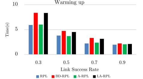
4.6 Network warming time test

Warming time for the first time. The warming time of the in each RPL network graph, the root node transmits start message, which is a rudimentary DIO message. Afterwards, the network requires an opportunity to create the network graph. As shown in Fig.l6, despite former favorable results of the proposed method, this method requires longer network proposed method consists of the restriction of the number of children assigned to the parent node and amalgamate it into DIO message format, as well as the priority comparison among child nodes for the purpose of selecting the best parent among all available parents. This procedure requires more incipient exchanges as compared to the base ap-proaches like RPL and A-RPL. The degree restriction of parent nodes increases the number of levels and effort steps passed by child nodes for the sake of parent node selection; therefore, the height of network tree has been increased. This approach has been regarded as desirability cost and routing management of network nodes, and, in accordance with the inevitable existence of both privileges and deficiencies in each proposed loT protocol, this can be alluded to as the cost of the proposed method. In addition, the effect of successful transmission rate of link on the warming time also indicates the efforts made by nodes, in order to create the network graph. According to Fig.16, in the proposed method of this paper, as the successful transmission rate of links decreases, the waiting time for the creation of network graph is in-creased up to four times. However, in RPL and A-RPL approaches, this increase trend has been up to at most three times. This observation highlights the significance of the link quality in the proposed method and BD-RPL approach.

Fig. 16. The comparison of warming time in network graph while the successful transmission rate of links

0 2 4 6 8

2 3 4 5

D

elay

U

p

war

d

(s)

Hop Upward Average Delay

RPL BD-RPL A-RPL LA-RPL

0 5 10

0.3 0.5 0.7 0.9

Tim

e(

s)

Link Success Rate Warming up

varies between 0.3 to 0.9.

Fig. 17. A perspective of the designed sensor node accompanied by ST-Link interface.

5.

PERFORMANCE

EVALUATION

IN

PRACTICAL

TESTS

For the sake of performance evaluation of the proposed method, some practical tests are performed in addition to the previously presented simulation tests. Note that practical tests are executed on the same designed hardware with the same conditions. A perspective of the designed sensor nodes in loT Laboratory is illustrated in Fig.17. Similarly, the distribution of nodes in indoor and outdoor environments are respectively shown in Fig.18 and Fig19.

Fig. 18. A perspective of nodes distribution in indoor environment.

Fig. 19. A perspective of nodes distribution in outdoor environment. 5.1 Routing packets and lost packets evaluation

Table 2

The results of practical tests comparing the proposed method and the base approaches in indoor and outdoor environ-ments.

Protocol Sent Receive Drop Aggregated (%)

RPL(Indoor) 81874 75313 6561 0

RPL(Outdoor) 81430 77987 3443 0

LA-RPL(Indoor) 83718 82665 1053 34.11

LA-RPL(Outdoor) 82880 82151 729 37.7

5.2 Average power consumption per node

This test is allocated to the investigation of the average energy consumption for each network node. In accordance with the acquired simulation results presented in Fig.12, it is observed through this practical test that the energy consumption of network nodes is reduced. According to Fig.20, the average energy consumption of each network node for traffic rates 5, 10, and 15 packets per minute is respectively 3.37, 6.14, and 17.4 millie-watts.

Fig. 20. Comparison of average energy consumption of each node, while the traffic rate is 5, 10, and 10 packets per mi-nute.

5.3 Average number of DIO control packets while topology changes

The main objective of this test is to investigate the extend to which the proposed method is effective to preserve trickle timer; such that the transmission of unnecessary DIO messages are avoided. In other words, through this test, it is inves-tigated that to what extend the creation of steady network graph can reduce the control overhead, and increase the available time of nodes as well. In the proposed method, through providing a balance in network graph, the degree restriction of parent nodes prevents the occurrence of congestion; therefore, the rate of DIS messages and network insta-bility is reduced in comparison with the base RPL approach. This is mainly due to the fact that despite the existence of upper-threshold recognized instability in the network, a reset trickle timer which culminates in the transmissions of DIO messages, as well as some changes in the network graph are essential. A consequential note in this test is that the location of five nodes have been changed after the passage of 60 minutes from the initial start time. This is done so as to investigate and compare both approaches in terms of both the speed and the cost of restoring network graph in indoor and outdoor environments. The acquired results of this test are resented in Fig.21

0 10 20 30 40

15 10 5

P owe r( m W )

Packet per Minute

Average Power Consumption per Node

RPL BD-RPL A-RPL LA-RPL

0 50 100 150 t=0 .1 t=1 0 t=2 0 t=3 0 t=4 0 t=5 0 t=6 0 t=7 0 t=8 0 t=9 0 t=1 00 t=1 10 t=1 20 N u m b er of D IO Time(Minute) Average Number of DIO

Fig. 21. The diagram of drop scheduler control of DIO message in indoor aud outdoor environments.

6.

CONCLUSION

Due to the significance of communications among nodes as well as the topology and data packets transmission method in wireless sensor networks, specifically in the Internet of Things, this research has investigated the state-of-the-art pro-posed methods and presented a novel solution for the mentioned issues. According to the presented documentaries in this research, routing approaches in IoT have extended facets, such that it is highly dependance on the hardware, soft-ware, and the embedded operating system leads to a number of various challenges. Routing efficiency of a destined source and destination pair is remarkably affected by issues such as computational overhead, algorithmic complexity, security, reliability, hardware fault tolerance, data error, and so forth. Such challenges are so wide-ranging and relevant to the cross-layer issues that exceed the scope of this research. This paper focuses on the reduction of both excessive exchanges and routing load in IoT, specifically in RPL approach. In the proposed method of this paper, through exerting graph degree restriction on each parent node, the exchange rate is reduced as far as possible to a cogent extent.

Furthermore, through the utilization of learning automata, packets belonging to similar directions are aggregated toward network root, and the time consumption is managed in terms of the data exchange rate. This approach yields in the more intelligent formation of the network graph, and more efficient load balancing in the network in both simulation and practical environments as a result. The accrued results from both simulations and practical tests results confirm the remarkably superior performance of the proposed method in terms of energy consumption, control overhead, and root access delay as compared to the previously proposed methods.

R

[1] S. Cirani, G. Ferrari, M. Picone, and L. Veltri, Internet of Things: Architectures, Protocols and Standards. John Wiley & Sons, 2018.

[2] F. Montori, L. Bedogni, and L. Bononi, “A collaborative internet of things architecture for smart cities and environmental monitoring,” IEEE Internet Things J., vol. 5, no. 2, pp. 592–605, 2018.

[3] B. N. Silva, M. Khan, and K. Han, “Internet of things: A comprehensive review of enabling technologies, architecture, and challenges,” IETE Tech. Rev., vol. 35, no. 2, pp. 205–220, 2018.

[4] F. Javed, M. K. Afzal, M. Sharif, and B.-S. Kim, “Internet of Things (IoT) Operating Systems Support, Networking Technologies, Applications, and Challenges: A Comparative Review,” IEEE Commun. Surv. Tutorials, vol. 20, no. 3, pp. 2062–2100, 2018.

[5] E. Fitzgerald, M. Pióro, and A. Tomaszewski, “Energy-optimal data aggregation and dissemination for the Internet of Things,” IEEE Internet Things J., vol. 5, no. 2, pp. 955–969, 2018.

[6] M. Hamzei and N. J. Navimipour, “Toward Efficient Service Composition Techniques in the Internet of Things,” IEEE Internet Things J., vol. 5, no. 5, pp. 3774–3787, 2018.

[7] B. Pourghebleh and N. J. Navimipour, “Data aggregation mechanisms in the Internet of things: A systematic review of the literature and recommendations for future research,” J. Netw. Comput. Appl., vol. 97, pp. 23–34, 2017.

[8] P. Sethi and S. R. Sarangi, “Internet of Things: Architectures, Protocols, and Applications,” J. Electr. Comput. Eng., vol. 2017, pp. 1–25, 2017. [9] C. Siu and K. Iniewski, “The Internet of Things—Physical and Link Layers Overview,” in IoT and Low-Power Wireless, CRC Press, 2018, pp. 33–

44.

[10] M. Lohstroh, H. Kim, J. C. Eidson, C. Jerad, B. Osyk, and E. A. Lee, “On Enabling Technologies for the Internet of Important Things,” IEEE Access, 2019.

[11] Y. Shen, T. Zhang, Y. Wang, H. Wang, and X. Jiang, “MicroThings : A Generic IoT Architecture for Flexible Data Aggregation and Scalable Service Cooperation,” IEEE Commun. Mag., vol. 55, no. 9, pp. 86–93, 2017.

[12] Z. Qin, D. Wu, Z. Xiao, B. Fu, and Z. Qin, “Modeling and Analysis of Data Aggregation From Convergecast in Mobile Sensor Networks for Industrial IoT,” IEEE Trans. Ind. Informatics, vol. 14, no. 10, pp. 4457–4467, 2018.

[13] X. Li, S. Liu, F. Wu, S. Kumari, and J. J. P. C. Rodrigues, “Privacy Preserving Data Aggregation Scheme for Mobile Edge Computing Assisted IoT Applications,” IEEE Internet Things J., 2018.

[14] H. Harb, A. Makhoul, S. Tawbi, and R. Couturier, “Comparison of different data aggregation techniques in distributed sensor networks,” IEEE Access, vol. 5, pp. 4250–4263, 2017.

[15] H. Jiang, F. Shen, S. Chen, K.-C. Li, and Y.-S. Jeong, “A secure and scalable storage system for aggregate data in IoT,” Futur. Gener. Comput. Syst., vol. 49, pp. 133–141, 2015.

[16] M. Uddin, S. Mukherjee, H. Chang, and T. V Lakshman, “SDN-Based Multi-Protocol Edge Switching for IoT Service Automation,” IEEE J. Sel. Areas Commun., vol. 36, no. 12, pp. 2775–2786, 2018.

[17] J. Mineraud, O. Mazhelis, X. Su, and S. Tarkoma, “A gap analysis of Internet-of-Things platforms,” Comput. Commun., vol. 89, pp. 5–16, 2016. [18] H. Sándor, B. Genge, and Z. Gál, “Security assessment of modern data aggregation platforms in the internet of things,” Int. J. Inf. Secur. Sci., vol.

4, no. 3, pp. 92–103, 2015.

[19] T. Zhu, S. Dhelim, Z. Zhou, S. Yang, and H. Ning, “An architecture for aggregating information from distributed data nodes for industrial internet of things,” Comput. Electr. Eng., vol. 58, pp. 337–349, 2017.

[20] S. Sirsikar and S. Anavatti, “Issues of data aggregation methods in wireless sensor network: A survey,” Procedia Comput. Sci., vol. 49, pp. 194– 201, 2015.

[21] G. Dhand and S. S. Tyagi, “Data aggregation techniques in WSN: Survey,” Procedia Comput. Sci., vol. 92, pp. 378–384, 2016.

[22] A. Bahramlou and R. Javidan, “Adaptive timing model for improving routing and data aggregation in Internet of things networks using RPL,” IET Networks, 2018.

[23] H.-S. Kim, J. Ko, D. E. Culler, and J. Paek, “Challenging the IPv6 Routing Protocol for Low-Power and Lossy Networks (RPL): A Survey,” IEEE Commun. Surv. Tutorials, vol. 19, no. 4, 2017.

[24] B. Ghaleb et al., “A Survey of Limitations and Enhancements of the IPv6 Routing Protocol for Low-power and Lossy Networks: A Focus on Core Operations,” IEEE Commun. Surv. Tutorials, 2018.

[25] X. Vilajosana, P. Tuset, T. Watteyne, and K. Pister, “OpenMote: Open-Source Prototyping Platform for the Industrial IoT,” in International Conference on Ad Hoc Networks, no. SEPTEMBER, Springer, 2015, pp. 211–222.

[27] W. Khallef, M. Molnar, A. Benslimane, and S. Durand, “Multiple constrained QoS routing with RPL,” in Communications (ICC), 2017 IEEE International Conference on, 2017, pp. 1–6.

[28] F. Boubekeur, L. Blin, R. Leone, and P. Medagliani, “Bounding Degrees on RPL,” in Proceedings of the 11th ACM Symposium on QoS and Security for Wireless and Mobile Networks, 2015, pp. 123–130.

[29] H.-S. Kim, H. Kim, J. Paek, and S. Bahk, “Load balancing under heavy traffic in RPL routing protocol for low power and lossy networks,” IEEE Trans. Mob. Comput., vol. 16, no. 4, pp. 964–979, 2017.

[30] M. Asemani and M. Esnaashari, “Learning automata based energy efficient data aggregation in wireless sensor networks,” Wirel. Networks, vol. 21, no. 6, pp. 2035–2053, Jan. 2015.

[31] A. Rezvanian, A. M. Saghiri, S. M. Vahidipour, M. Esnaashari, and M. R. Meybodi, Recent advances in learning automata. Springer, 2018. [32] M. Ahmadinia, H. Alinejad-Rokny, and H. Ahangarikiasari, “Data aggregation in wireless sensor networks based on environmental similarity: A

learning automata approach,” J. Networks, vol. 9, no. 10, p. 2567, 2014.

[33] O. Hahm, E. Baccelli, H. Petersen, and N. Tsiftes, “Operating systems for low-end devices in the internet of things: a survey,” IEEE Internet Things J., vol. 3, no. 5, pp. 720–734, 2016.