SANJIT CHATTERJEE, DARREL HANKERSON, EDWARD KNAPP, AND ALFRED MENEZES
Abstract. In 2003, Boneh, Gentry, Lynn and Shacham (BGLS) devised the first provably-secure aggregate signature scheme. Their scheme uses bilinear pairings and their security proof is in the random oracle model. The first pairing-based aggregate signature scheme which has a security proof that does not make the random oracle assumption was proposed in 2006 by Lu, Ostrovsky, Sahai, Shacham and Waters (LOSSW). In this paper, we compare the security and efficiency of the BGLS and LOSSW schemes when asymmetric pairings derived from Barreto-Naehrig (BN) elliptic curves are employed.
1. Introduction
Beginning with the work of Joux [27] in 2000, bilinear pairings have been extensively used to design cryptographic protocols. Bilinear pairings come in two flavours – symmetric and asymmetric. Ifnis prime, andGandGT are two groups of ordern, then asymmetric pairing on (G,GT) is a functione:G×G→GT
that is bilinear, non-degenerate, and efficiently computable. Following [17], we will refer to these pairings as
Type 1 pairings. On the other hand, if G1,G2 andGT are three groups of ordern withG16=G2, then an
asymmetric pairing on (G1,G2,GT) is a function e: G1×G2 →GT that is bilinear, non-degenerate, and
efficiently computable. Following [17], asymmetric pairings for which an efficiently-computable isomorphism ψ : G2 → G1 is known will be called Type 2 pairings, while asymmetric pairings for which no efficiently-computable isomorphism is known either fromG1to G2 or fromG2 toG1are called Type 3 pairings.
Boneh, Lynn and Shacham [9] were the first to observe that an efficiently-computable isomorphismψfrom G2 to G1 can be essential to the security of a protocol. They showed that their short-signature scheme is insecure if implemented with a certain bilinear pairing for which the co-Diffie-Hellman problem (co-DHP; see
§2.3 for the definition of co-DHP) is intractable but for which an isomorphismψis not known. Boneh, Lynn and Shacham commented that the requirement for the mapψcan be avoided by using a Type 3 pairing at “the cost of making a stronger complexity assumption”, namely that co-DHP* is intractable (see§2.3 for the definition of co-DHP*). They conclude by saying that sinceψ naturally exists in Type 2 pairings, there is no reason to rely on this stronger complexity assumption. It is perhaps because of the prevailing belief that hardness of co-DHP* is a stronger complexity assumption than hardness of co-DHP that most researchers who describe their protocols with asymmetric pairings use Type 2 pairings instead of Type 3 pairings.
In this paper we compare the security and efficiency of two provably-secure pairing-based signature schemes — those of Boneh, Gentry, Lynn and Shacham (BGLS) [7] and Lu, Ostrovsky, Sahai, Shacham and Waters (LOSSW) [29]. The BGLS scheme was originally described using the setting of a Type 2 pairing, and its security proof is in the random oracle model (ROM). The LOSSW scheme, on the other hand, was described in the setting of a Type 1 pairing, and its security proof did not make the random oracle assumption. The authors of [29] claimed that the LOSSW scheme “in some cases outperform[s] the most efficient random-oracle-based schemes”, and in particular has faster signature verification than BGLS. The basis for the latter claim was that a BGLS signature verification requiresℓ+1 pairing computations whenℓsignatures have been aggregated, whereas LOSSW requires only 2 pairing computations. However, the removal of the relatively-expensive pairing operations is at the expense of introducing other operations including multiplications,
Date: February 24, 2009; revised on August 15, 2009 and on September 22, 2009.
exponentiations, and group membership testing, and possibly requiring larger public keys and signatures. Our goal in this paper is a detailed comparison of BGLS and LOSSW using state-of-the-art BN pairings, and by using the known reductionist security arguments to guide the protocol specification and parameter selection.
We show that the BGLS and LOSSW schemes, as well as the BLS [9] and Waters [41] signature schemes upon which they are based, can all be described using Type 3 pairings (and that the Waters and LOSSW schemes can be described using Type 2 pairings).1 We explain how some of these protocols have to be modified in order for the known reductionist security proofs to carry over to the different settings.2 We argue, contrary to what can be inferred from [9], that the existing evidence suggests that Type 3 pairings offer at least as much security as Type 2 pairings when used to implement the four signature schemes under consideration. Furthermore, we compare Type 2 and Type 3 pairings derived from a certain Barreto-Naehrig (BN) elliptic curve [2] offering 128 bits of security. We show that the elements of the groupG2 in Type 2 pairings can always be represented so that operations in G2 have significantly lower cost than suggested by the high-level estimates of Galbraith, Paterson and Smart [17] and the analysis of Chen, Cheng and Smart [12]. Despite these improvements, we conclude that Type 2 pairings offer no performance benefits over Type 3 pairings. Finally, we demonstrate that the BGLS scheme outperforms the LOSSW scheme in every respect — smaller public keys, smaller signatures, faster signature generation, and faster signature verification when 10 or fewer signatures have been aggregated.
The remainder of this paper is organized as follows. The construction of Type 2 and Type 3 pairings from BN curves are reviewed in§2, and their security is contrasted. In§3, we describe a particular BN curve and offer concrete estimates of the efficiency of fundamental operations in the Type 2 and Type 3 pairings derived from this curve. The security and efficiency of the BLS and Waters signature schemes are compared in §4. Finally,§5 compares the security and efficiency of the BGLS and LOSSW aggregate signature schemes.
Notation. In order to maintain consistency with the literature, G, G1, G2, G′2 will be additively-written cyclic groups with generators P, P1, P2, P′
2 in §2 and §3, while in §4 and §5, G, G1, G2, G′2 will be multiplicatively-written cyclic groups with generatorsg, g1, g2, g′
2. The notation SIG-x is used to denote the signature scheme SIG implemented with a Type x pairing, where x∈ {1,2,3}.
2. Barreto-Naehrig curves
Barreto-Naehrig elliptic curves [2] are parameterized by an integerzfor which bothp(z) = 36z4+ 36z3+ 24z2+ 6z+ 1 andn(z) = 36z4+ 36z3+ 18z2+ 6z+ 1 are prime. For each suchz, there is an ordinary elliptic curve E : Y2 =X3+b defined over the finite fieldF
p where p=p(z), and such that #E(Fp) =n where
n=n(z). Such an elliptic curve has embedding degreek= 12, this being the smallest positive integer for whichndividespk−1. If follows thatE[n]⊆E(F
p12), whereE[n] denotes the set of alln-torsion points on
E. (Recall thatE[n] is a finite abelian group of rank 2, whenceE[n]∼=Zn⊕Zn andE[n] hasn+ 1 different
subgroups of ordern.)
2.1. Type 3 pairings from BN curves. LetG1=E(Fp), and letGT denote the unique order-nsubgroup
of F∗
p12. Now, E has a sextic twist over Fp2, namely ˜E/Fp2 : Y2 = X3+b′, such that n | # ˜E(Fp2) and
n2∤# ˜E(Fp2) [24]. Let ˜T ∈E˜(Fp2) be a point of ordern, and define ˜G2=hT˜i. Then there is an
efficiently-computable monomorphismφ: ˜E(Fp2)→E(Fp12). Letting T =φ( ˜T) and G2=hTi, we haveG26=G1 and
an efficiently-computable group isomorphismφ: ˜G2 →G2. The groupG2 is called thetrace-0 subgroup of
1Type 1 pairings are currently viewed as being significantly slower than their Type 2 and Type 3 counterparts (see [22]) at
the 128-bit security level, and therefore we will restrict our attention in this paper to Type 2 and Type 3 pairings.
2Smart and Vercauteren [40] analyzed the security of the BLS signature scheme in the Type 3 setting. Their security
E[n] since it has the property that Tr(Z) = P11
i=0πi(Z) = ∞ for allZ ∈ G2, whereπ : (x, y)7→ (xp, yp) is the pth-power Frobenius map. We next define three asymmetric pairings on (G1,G2,GT). Since no
efficiently-computable isomorphism fromG1toG2 or fromG2toG1 is known, these pairings are of Type 3. The (full) Tate pairing ˆe : E[n]×E[n] → GT can be defined as follows. Let P, Q ∈ E[n], and let
R∈E(Fp12) withR6∈ {∞, P,−Q, P −Q}. Then
ˆ
e(P, Q) =
f
n,P(Q+R)
fn,P(R)
(p12−1)/n
,
where the Miller function fs,P is a function whose only zeros and poles in E are a zero of order sat P, a
pole of order 1 atsP, and a pole of orders−1 at∞. The (restricted) Tate pairing tn:G1×G2→GT is
defined by
tn(P, Q) = (fn,P(Q))(p
12
−1)/n
, and can be computed using Algorithm 1.
Algorithm 1(Computing the Tate pairing)
Input:P ∈G1 andQ∈G2.
Output:tn(P, Q).
1. Writenin binary: n=PL−1
i=0 ni2i. 2. T←P, f←1.
3. ForifromL−2 downto to 0 do: {Miller operation}
3.1 Letℓbe the tangent line atT. 3.2 T←2T, f←f2·ℓ(Q). 3.3 Ifni = 1 andi6= 0 then
Letℓbe the line throughT and P. T←T+P, f←f·ℓ(Q).
4. Return(f(p12
−1)/n). {Final exponentiation}
Theate pairing an:G1×G2→GT, introduced by Hess, Smart and Vercauteren [24], is defined by
an(P, Q) = (ft−1,Q(P))(p
12
−1)/n
where t−1 = p−#E(Fp) = 6z2. The ate pairing is generally faster to compute than the Tate pairing
because the number of iterations in the Miller operation is determined by the bitlength oft−1≈√n. TheR-ate pairing Rn:G1×G2→GT, introduced recently by Lee, Lee and Park [28], further decreases
the number of iterations of the Miller operation. It is defined by
Rn(P, Q) = f·(f·ℓaQ,Q(P))p·ℓπ(aQ+Q),aQ(P)
(p12−1)/n
,
where a = 6z + 2, f = fa,Q(P), and ℓA,B denotes the line through A and B. There is an integer N
such thatRn(P, Q) = ˆe(Q, P)N for allP ∈G1 andQ∈G2 [28]. The R-ate pairing can be computed using Algorithm 2. Notice that the number of iterations in the Miller operation is now determined by the bitlength ofa≈√t≈n1/4.
Algorithm 2(Computing the R-ate pairing)
Input:P ∈G1 andQ∈G2.
Output:Rr(Q, P).
1. Writea= 6z+ 2 in binary: a=PL−1
2. T←Q, f←1.
3. ForifromL−2 downto 0 do: {Miller operation}
3.1 Letℓbe the tangent line atT. 3.2 T←2T, f←f2·ℓ(P). 3.3 Ifai = 1 then
Letℓbe the line throughT and Q. T←T+Q, f←f·ℓ(P).
4. f←f·(f ·ℓT,Q(P))p·ℓπ(T+Q),T(P).
5. Return(f(p12
−1)/n). {Final exponentiation}
Table 1 from [22] lists the costs of computing the Tate, ate, and R-ate pairings for a particular BN curve described in§3, demonstrating the superiority of the R-ate pairing. The cost estimates have been validated by experiments. For example, [22] reports timings of 81 million and 54 million clock cycles for computing the ate and R-ate pairings on a 2.8 GHz Pentium 4 machine using general purpose registers.
Pairing Miller operation Final exponentiation Total Tate 27,934m 7,246m+i 35,180m+i
ate 15,801m 7,246m+i 23,047m+i
R-ate 7,847m+i 7,246m+i 15,093m+2i
Table 1. Costs of the Tate, ate and R-ate pairings for the BN curve described in§3. Here, mandidenote multiplication and inversion inFp.
If the product ofℓ R-ate pairings is desired, then the steps of the individual pairing computations can be interleaved, with the product of the partial results being stored in a common accumulatorf [38, 21]. In that case, the expensive operationf←f2 in step 3.2 of Algorithm 2 and the final exponentiation in step 5 can be shared by all ℓ pairing computations. It follows that the cost of computing the product ofℓ R-ate pairings for the particular BN curve is 15,093m+ 2i+ (ℓ−1)(5507m+i); i.e., the incremental cost of each additional pairing is roughly one-third the cost of the first pairing.
2.2. Type 2 pairings from BN curves. Let R∈E[n] withR 6∈G1 andR 6∈G2, and define G′2=hRi. Then the mapen:G1×G′2→GT defined byen(P, Q) = ˆe(Q, P)2N is an asymmetric pairing on (G1,G′2,GT).
It is a Type 2 pairing because the trace map Tr is an efficiently-computable isomorphism fromG′
2 toG1. At first glance, it may appear that evaluating en(P, Q) may be more expensive than evaluating the
Type 3 pairingRnbecause the pointQ∈G′2has coordinates that are inFp12and not in any proper subfield.
However, the following shows that the task of computingen(P, Q) is easily reduced to the task of computing
an R-ate pairing value.
Lemma 1([25]). Let P ∈G1 andQ∈G′2. Then en(P, Q) =Rn(P,Qˆ), whereQˆ=Q−π6(Q).
Proof. First note that ˆQ6=∞since Q6∈E(Fp6). Moreover, Tr( ˆQ) = Tr(Q)−Tr(π6(Q)) =∞, and hence
ˆ
Q∈G2. Finally,
en(P, Q) = eˆ(Q, P)2N
= eˆ(2Q, P)N
= eˆ(Q+ ˆQ+π6(Q), P)N = eˆ( ˆQ, P)N·eˆ(Q+π6(Q), P)N = Rn(P,Qˆ),
sinceQ+π6(Q)∈E(F
2.3. Security. Recall that G1 =E(Fp), G2 is the trace-0 subgroup ofE[n], G′2 is any order-n subgroup of E[n] different from G1 and G2, and GT is the order-nsubgroup of F∗p12. BN curves are especially well
suited for the 128-bit security level because if pis a 256-bit prime (whence nis also a 256-bit prime) then Pollard’s rho method [34] for computing discrete logarithms inG1,G2, G′2 orGT has running time at least
2128, as does the number field sieve algorithm for computing discrete logarithms in the extension fieldF
p12
[19, 35, 36]. Schirokauer [37] has shown that there are cases where discrete logarithms in prime fieldsFpand
degree-two extensionsFp2 of prime fields can be computed significantly faster than standard versions of the
number field sieve if the primephas low Hamming weight. However, Schirokauer’s method is not known to be effective for computing discrete logarithms inFp12 for BN primesp, even if the BN parameterz is chosen
so thatphas relatively small Hamming weight. Thus, the fastest algorithms presently known for computing discrete logarithms inG1,G2,G′2 andGT have running times at least 2128.
It should be noted that while the discrete logarithm problems in the groups G1, G2, G′2 and GT are
equivalent in practice, such an equivalence has never been proven. Let us denote the discrete logarithm problem in a groupGby DLPG. The Tate pairing can be used to efficiently reduce the DLP in any order-n subgroup of E[n] to the DLP in GT. Namely, if P ∈ E[n] and Q ∈ hPi, then one has logPQ = logαβ
where α = ˆe(P, R), β = ˆe(Q, R), and R ∈ E[n] is chosen so that ˆe(P, R) 6= 1. Now, the trace map Tr :G′
2→ G1 is an efficiently-computable isomorphism and so DLPG′
2 ≤DLPG1. Furthermore, if Q∈G′2
thenQ2=Q− 1
12Tr(Q)∈G2 sinceQ2∈E[n] and Tr(Q2) = Tr(Q)−Tr(Q) =∞. Hence the map
(1) ρ:G′
2→G2, Q7→Q− 1 12Tr(Q) is an efficiently-computable isomorphism, whence DLPG′
2 ≤DLPG2. Figure 1 summarizes the known
rela-tionships between the DLP inG1, G2,G′2andGT.
DLPG2
DLPG 1
co-DHP DLPG′
2
co-DHP* DLPG
T
Figure 1. Relative difficulty of the discrete logarithm problems in G1, G2, G′2, GT, and
the co-DHP and co-DHP* problems. The notationA←B means that there is an efficient reduction fromA to B. The equivalence of co-DHP* and co-DHP holds if the generators P1,P2,P′
2 are suitably chosen (cf. Lemma 2).
Suppose now thatP1, P2, P′
2 are fixed generators of G1, G2, G′2, respectively. Security of the signature schemes considered in §4 and §5 is based on a variant of the Diffie-Hellman problem (DHP). (Recall that DHP in a group G = hPi is the problem of determining xyP given xP and yP.) If a Type 2 pairing is employed, then security of the signature schemes is based on the hardness of co-DHP: Given Q∈G1 and zP′
2 ∈G′2, compute zQ. The intractability of DLPG′
2 is a necessary condition for hardness of co-DHP. On
the other hand, if a Type 3 pairing is employed, then security is based on the hardness ofco-DHP*: Given Q, zP1 ∈G1 andzP2 ∈G2, compute zQ. The intractability of DLPG1 and DLPG2 are both necessary for
the hardness of co-DHP*.
the case of the DLP and DHP in a prime-order group, it has not been proven that the hardness of co-DHP and co-DHP* is independent of the choice of generators.
It is not known whether DLPG1 ≤ co-DHP*, or DLPG2 ≤ co-DHP*, or DLPG′2 ≤ co-DHP. This is
unlike the case of the DHP in an order-ngroupG, where there is substantial evidence that DLPG≤DHPG. For example, den Boer [5] proved that DLPG ≤DHPG if the group ordern has the property thatn−1 is smooth. Furthermore, den Boer’s result was extended by Boneh, Lipton and Maurer [8, 30] to the case where an elliptic curve overZn of smooth order is known. Consequently, concerns that DHPGmight be easier than
DLPG can be alleviated by selecting an order-ngroupG for which the appropriate elliptic curves overZn
are known [31]. The techniques of den Boer, Boneh, Lipton and Maurer do not appear to extend to the case of co-DHP and co-DHP*, and consequently there is presently no evidence (in the form of a reduction) that these problems are equivalent to the DLP inG1,G2or G′2.
The following shows that co-DHP and co-DHP* are equivalent if the generatorsP1, P2, P′
2 are suitably chosen.
Lemma 2. Let P′
2 ∈ E[n] be an arbitrary point with P2′ 6∈ G1 and P2′ 6∈ G2, and let G′2 = hP2′i. Let c ∈ [1, n−1] be an arbitrary integer, and define P2 =c−1ρ(P′
2) and P1 = 121 Tr(P2′). If c is known, then
co-DHP≤co-DHP* and co-DHP*≤co-DHP.
Proof. Note thatP′
2=P1+cP2. It can easily be checked thatP1∈G1\ {∞}andP2∈G2\ {∞}. Now, given a co-DHP instance (Q, zP′
2), we computec−1ρ(zP2′) =zP2andzP2′−czP2=zP1. A co-DHP* solver is then used to find the solution zQof the co-DHP* instance (Q, zP1, zP2), thus also obtaining the solution to the original co-DHP instance. This shows that co-DHP≤co-DHP*.
Conversely, given a co-DHP* instance (Q, zP1, zP2), we computezP1+czP2=zP′
2. A co-DHP solver is then used to find the solutionzQof the co-DHP instance (Q, zP′
2), thus also obtaining the solution to the
original co-DHP* instance. This shows that co-DHP*≤co-DHP.
It is not known whether knowledge of the integer c makes co-DHP or co-DHP* any easier. Suppose instead thatP2 and P′
2 were chosen independently at random fromG2 and E[n]\(G1∪G2), respectively, and P1 = 1
12Tr(P2′). In this scenario, the integer c satisfying ρ(P2′) =cP2 is not known, and we do not know efficient reductions from co-DHP to co-DHP* or from co-DHP* to co-DHP. The fact that efficient reductions DLPG′
2 ≤DLPG1 and DLPG′2 ≤DLPG2 are known, while efficient reductions DLPG1 ≤DLPG′2
and DLPG2 ≤ DLPG′2 are not known, might cause some people to have more confidence in the hardness
of DLPG1 and DLPG2 than of DLPG′2, and consequently more confidence in hardness of co-DHP* than of
co-DHP. One should also note that the Decisional DHP is easy in G′
2, but not known to be easy in G1 or inG2 [6]. Thus, the existing evidence does not indicate any weakness in Type 3 pairings relative to Type 2 pairings, but rather that Type 3 pairings are at least as secure as Type 2 pairings.
2.4. Representation of G′
2. In the remainder of the paper, we shall assume that G′2 = hP2′i where the pointP′
2was selected at random fromE[n]\(G1∪G2). Furthermore, we chooseP1=121 Tr(P2′), whence
(2) ψ:G′
2→G1, Q7→ 1 12Tr(Q) is an efficiently-computable isomorphism such thatψ(P′
2) =P1. We either setP2=c−1ρ(P2′) for an arbitrary integerc∈[1, n−1] (in which case co-DHP and co-DHP* are provably equivalent), or setP2to be a randomly selected trace-0 point (in which case it is not known how to prove the equivalence of co-DHP and co-DHP*).
Given Q∈G′
2, one can efficiently determine the uniqueQ1 ∈G1 andQ2 ∈G2 such thatQ=Q1+Q2; namely,Q1=ψ(Q) andQ2=ρ(Q) =Q−Q1. Writing
(3) D(Q) = (ψ(Q), ρ(Q)),
and lettingH′
2⊆G1×G2denote the range ofD, we have an efficiently-computable isomorphismD:G′2→H′2 whose inverse is also efficiently computable. Note that addition inH′
We note that Smart and Vercauteren [40] had previously proposed defining a pairing where the groupG′
2 was taken to be an order-nsubgroup of G1×G2. Our observation is that such a representation is without loss of generality, i.e., it can be used forall order-nsubgroupsG′
2 ofE[n] different fromG1 andG2.
3. A particular BN curve
For the remainder of this paper, we will work with the BN curve
E/Fp:Y2=X3+ 3
with BN parameter z= 6000000000001F2D (in hexadecimal) [14]. For this choice of BN parameter,pis a 256-bit prime of Hamming weight 87,n= #E(Fp) is a 256-bit prime of Hamming weight 91,t−1 = 6z2 is
a 128-bit integer of Hamming weight 28, and the R-ate parametera= 6z+ 2 is a 66-bit integer of Hamming weight 9. Note thatp≡7 (mod 8) (whence−2 is a nonsquare modulop) andp≡1 (mod 6).
3.1. Field representation. The extension fieldFp12 is represented using tower extensions
Fp2 = Fp[u]/(u2+ 2),
Fp6 = Fp2[v]/(v3−ξ) whereξ=−u−1, and
Fp12 = Fp6[w]/(w2−v).
We also have the representation
Fp12 =Fp2[W]/(W6−ξ) whereW =w.
Hence an elementα∈Fp12 can be represented in any of the following three ways:
α=a0+a1w where a0, a1∈Fp6
= (a0,0+a0,1v+a0,2v2) + (a1,0+a1,1v+a1,2v2)w whereai,j∈Fp2
=a0,0+a1,0W+a0,1W2+a1,1W3+a0,2W4+a1,2W5.
We let (m, s, i), ( ˜m,˜s,˜ı), (M, S, I) denote the cost of multiplication, squaring, inversion inFp, Fp2, Fp12,
respectively. Experimentally, we have s ≈0.9m and i ≈41m on a Pentium 4 processor [22]. In our cost estimates that follow, we will make the simplifying assumptions≈m.
3.1.1. Arithmetic in Fp2. We have ˜m ≈ 3m using Karatsuba’s method which reduces a multiplication in
a quadratic extension to 3 (rather than 4) small field multiplications; ˜s≈2m using the complex method: (a+bu)2= (a−b)(a+ 2b)−ab+ (2ab)u; and ˜ı≈i+ 2m+ 2ssince (a+bu)−1= (a−bu)/(a2+ 2b2). Note also thatp-th powering is free inFp2 because (a+bu)p=a−bu.
3.1.2. Arithmetic in Fp6. Karatsuba’s method reduces a multiplication in a cubic extension to 6 (rather
than 9) multiplications in the smaller field. Hence a multiplication in Fp6 costs 18m. Squaring in Fp6
costs 2 ˜m+ 3˜s = 12m via the following formulae [13]: if β = b0+b1v+b2v2 ∈ F
p6 where bi ∈ Fp2, then
β2 = (A+Dξ) + (B+Eξ)v+ (B+C+D−A−E)v2 where A = b2
0, B = 2b0b1, C = (b0−b1+b2)2, D= 2b1b2, andE=b2
2. Finally, as shown in [39, Section 3.2], inversion inFp6 can be reduced to 1 inversion,
9 multiplications, and 3 squarings inFp2.
3.1.3. Arithmetic in Fp12. SinceFp12 is a tower of quadratic, cubic, and quadratic extensions, Karatsuba’s
method givesM ≈54m. By using the complex method for squaring inFp12 and Karatsuba for multiplication
in Fp6 andFp2, we have S≈36m. Since inversion inFp12 can be reduced to 1 inversion, 2 multiplications,
3.1.4. Sextic twist. The sextic twist ˜E ofEoverFp2 for whichn|# ˜E(Fp2) is
˜
E/Fp2 :Y2=X3+ 3/ξ.
The monomorphismφ: ˜E(Fp2)→E(Fp12) is given by (x, y)7→(xW2, yW3). Thus the group isomorphism
φ: ˜G2→G2as well as its inverse can be computed at no cost.
3.2. Elliptic curve operations. A point (X, Y, Z) in jacobian coordinates corresponds to the point (x, y) in affine coordinates withx=X/Z2andy=Y /Z3. The formulas for doubling a point inE(F
pd) represented in jacobian coordinates require 3 multiplications and 4 squarings in Fpd, while the formulas for mixed jacobian-affine addition inE(Fpd) require 8 multiplications and 3 squarings inFpd.
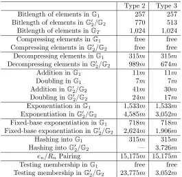
3.3. Type 2 versus Type 3 pairings. Table 2 lists the bitlengths of elements in G1, G2, G′2 and GT,
and the estimated costs of performing essential operations in these groups. Our estimates are consistent with the high-level comparisons in Table 3 of [17] and Table 5 of [12], with the notable exception that the representation we use forG′
2 results in elements of significantly smaller bitlengths and significantly faster exponentiation.3
Type 2 Type 3 Bitlength of elements inG1 257 257 Bitlength of elements inG′
2/G2 770 513
Bitlength of elements inGT 1,024 1,024
Compressing elements inG1 free free Compressing elements inG′
2/G2 free free
Decompressing elements inG1 315m 315m Decompressing elements inG′
2/G2 989m 674m
Addition inG1 11m 11m
Doubling inG1 7m 7m
Addition inG′
2/G2 41m 30m
Doubling inG′
2/G2 24m 17m
Exponentiation inG1 1,533m 1,533m Exponentiation inG′
2/G2 4,585m 3,052m Fixed-base exponentiation inG1 718m 718m Fixed-base exponentiation inG′
2/G2 2,624m 1,906m
Hashing intoG1 315m 315m
Hashing intoG′
2/G2 — 3,726m
en/Rn Pairing 15,175m 15,175m
Testing membership inG1 free free Testing membership inG′
2/G2 23,775m 3,052m
Table 2. Bitlengths of elements inG1, G2, G′2 and GT, and estimated costs (in terms of
Fp multiplications) of basic operations.
3For example, Table 5 of [12] estimates the cost exponentiation inG′
2as 45 times the cost of exponentiation inG1; our ratio
3.3.1. Representing elements in G1, G2, G′2 and GT. A point Q = (x, y) ∈ G1 can be represented in compressed form by x ∈ Fp plus a sign bit ofy ∈ Fp. The full y-coordinate can be recovered by solving
y2=x3+ 3 overF
pviay=± √
x3+ 3 = (x3+ 3)(p+1)/4. The exponentiation can be performed using sliding windows of width 5, at a cost of 315m.
A pointQ∈G2has preimage (x, y)∈G˜2under φ−1and thus can be represented in compressed form by x∈Fp2 plus a sign bit of y ∈Fp2. The fully-coordinatey =±
p
x3+ 3/ξ can be recovered at a cost of 2 square roots inFpplusi+m+ 2susing Scott’s method for computing square roots inFp2 [39]. The overall
cost is 674m.
As noted in§2.4, a pointQ= (x, y)∈G′
2can be represented by the pair of pointsD(Q) = (Q1, Q2)∈H′2, where Q1 = 1
12Tr(Q) and Q2 = Q−Q1. Now, π
i(Q) for 1 ≤ i ≤ 5 can be computed by successive
application of π, each of which costs 30m sincep-th powering of an element in Fp12 costs 15m [22]. And,
since p6-th powering in F
p12 is free, πi(Q) for 6 ≤ i ≤ 11 can thereafter be obtained for free. Then
computing Tr(Q) =P11
i=0πi(Q) takes 11 additions inE(Fp12), after which computing 1
12Tr(Q) requires one exponentiation in G1. Finally, determining Q−Q1 requires one addition in E(Fp12). The overall cost of
deriving the representation (Q1, Q2) from Q is 8,163m. Recovering Qfrom (Q1, Q2) requires an addition in E(Fp12) at a cost of (at most) 540m. We will henceforth identify G′2 and H′2 and assume that points
in G′
2 are represented as (Q1, Q2). Such points can be compressed by compressing Q1 and Q2, while the decompression cost is 989m. Point addition and doubling can be done component-wise, at a cost of 41mand 24m, respectively.
Lastly, elements inGT can be compressed from 3072 bits to 1024 bits using the techniques described in
[20]. We will ignore theGT compression and decompression costs in our performance analysis of signature
schemes as they are a negligible portion of overall costs.
3.3.2. Exponentiation in G1, G2 and G′2. Computing kQ (also known as point multiplication), wherek is an integer andQis an elliptic curve point, can be performed using thew-NAF method. The expected cost of this method withℓ-bit exponentsk is
1D+ (2w−2−1)A+ ℓ
w+ 1A+ℓD,
whereDis the cost of doubling an elliptic curve point andAis the cost of adding two elliptic curve points (see [23, Algorithm 3.36]). However, faster exponentiation can be achieved using the Gallant-Lambert-Vanstone (GLV) strategy [18].
Let β ∈ Fp be an element of order 3 in Fp. Then λ : (x, y) 7→ (βx, y) is an efficiently-computable
endomorphism of E defined overFp. The GLV strategy computes kQ as k1Q+k2λ(Q) where k1 and k2
are half-length exponents. If interleaving is used to compute k1Q and k2λ(Q), and if k1 and k2 are each represented in width-wNAF, then the expected cost of exponentiation in G1 is approximately
2 1D+ (2w−2
−1)A
+ ℓ
w+ 1A+ ℓ 2D. Takingw= 5 yields a cost of 1,533m.
Galbraith and Scott [16] presented a 4-dimensional GLV strategy for exponentiation inG2. If interleaving is used to compute the four exponentiations, and the quarter-length exponents are represented in width-w NAF, then the expected cost of exponentiation inG2 is approximately
4 1D+ (2w−2
−1)A
+ ℓ
w+ 1A+ ℓ 4D. Takingw= 4 yields a cost of 3,052m.
Lastly, exponentiation of a point (Q1, Q2) inG′
Algorithm 3.45]) with windows of widthwhas expected cost approximately
2w−1
2w 2e−1
A+ (e−1)D,
where d=⌈ℓ/w⌉ande=⌈d/2⌉. Taking w= 5 yields the expected costs 718mand 1,906mfor fixed-base exponentiation inG1 andG2, respectively. As before, fixed-base exponentiation inG′2 can be performed as (kQ1, kQ2); the cost is 2,624m.
3.3.3. Hashing intoG1,G2 andG′2. Hashing intoG1 can be defined by first using a standard hash function (such as SHA-2) to hash to anx-coordinate ofE(Fp). Ay-coordinate can then be computed as
√
x3+ 3. The dominant cost is for computing the square root inFp, yielding our cost estimate of 315m for hashing
intoG1.
Hashing into G2 can be defined by first using a standard hash function to hash to an x-coordinate of ˜
E(Fp2), then computing ay-coordinate as p
x3+b/ξ∈F
p2, and finally multiplying the resulting point by
# ˜E(Fp2)/n to obtain a point of order n. Since square roots in Fp2 cost 674m and point multiplication
in ˜E(Fp2) costs 3,052m, hashing into G2 can be performed at a cost of 3,726m. The alternate hashing
technique of Galbraith and Scott [16] has approximately the same cost for our particular BN curve, but uses less memory.
As noted in [17], no efficient method is known for hashing intoG′
2. More precisely, what is meant is that no efficient hash function is known for which computing the discrete logarithms of hash values (to the base of the fixed generatorP′
2) is infeasible. This condition is imposed in order to eliminate from consideration the hash functions that first map a message to an integer z in the interval [0, n−1], and thereafter define the hash value to be zP′
2. All signature schemes considered in this paper would be insecure if such hash functions were employed.
3.3.4. Pairing. As Lemma 1 explains, a Type 2 pairingen(P, Q) can be reduced to a Type 3 pairingRn(P,Qˆ),
where ˆQ=Q−π6(Q). Given the representation (Q1, Q2) ofQ, we haveπ6(Q) =π6(Q1+Q2) =π6(Q1) + π6(Q2) = Q1−Q2. Hence ˆQ = (∞,2Q2) and so computing ˆQ requires only one doubling in G
2. For simplicity, we will use the same cost estimate of 15,175mfor computingen andRn.
3.3.5. Testing membership inG1,G2,G′2. Our descriptions of the signature schemes implicitly assume that all signature components are valid, i.e., belong to the appropriate group. Since the reductionist security proofs for these schemes require that signature components be valid, it seems prudent that the signature schemes include the validity checks. (However, we should mention that no attacks of the signature schemes have been reported in the literature if the validity checks are omitted.) For example, in the BLS-2 signature scheme (see §4.1.1) a verifier should first confirm that the signature σ is indeed an element of G1 before proceeding with the verification, while in Waters-2b (see§4.2.3) the verifier should first confirm thatα∈G1 and β ∈G′
2. Note that testing membership of public key elements needs to be performed only once by a certification authority who issues certificates for public keys.
For the BN curve under consideration, testing membership of a pointQinG1is very efficient, and simply amounts to verifying thatQ belongs to E(Fp). This costs a small number of Fp multiplications, which we
will henceforth take as ‘free’. Testing membership of a point Qin G2 involves a fast check thatφ−1(Q) is in ˜E(Fp2), followed by an exponentiation inG2 to verify thatnQ=∞. Testing membership of (Q1, Q2) in
G′
2 is more costly — it can be done by first verifying thatQ1 ∈G1 andQ2 ∈G2, and finally testing that Rn(Q1, T2) =Rn(T1, Q2), where D(P2′) = (T1, T2) can be precomputed. The total cost is 23,775m.
4.1. BLS signature scheme. The Boneh-Lynn-Shacham (BLS) signature scheme [9] is notable because signatures can be considerably shorter than ElGamal-type signatures. The scheme was described in [9] in the setting of Type 1 and Type 2 pairings.
4.1.1. BLS-2 signature scheme. Let e : G1×G′2 → GT be a Type 2 pairing, let ψ : G′2 → G1 be an efficiently-computable isomorphism withψ(g′
2) =g1, and letH:{0,1}∗→G1be a hash function. Alice’s private key is an integerx∈R[1, n−1], while her public key isX = (g′
2)x. To sign a message M, Alice computesh=H(M) andσ=hx. Her signature onM isσ. To verify the signed message (M, σ), Bob
computesh=H(M) and accepts if and only ife(σ, g′
2) =e(h, X). Correctness of the verification algorithm follows because
e(σ, g′
2) =e(hx, g′2) =e(h,(g2′)x) =e(h, X).
The following security result was proven in [9]. We present an informal outline of a proof that contains the essential ideas behind the conventional reductionist security argument. Recall that a signature scheme is said to besecure if it is existentially unforgeable under an adaptive chosen-message attack by a computationally bounded adversary.
Theorem 1. If co-DHP in(G1,G′
2)is hard, and H is a random function, then the BLS-2 signature scheme
is secure.
Argument. The adversaryA is given a public keyX ∈G′
2 and a signing oracle. Because of the assumption regarding randomness of the hash function, the choice of messages that A submits to the signing oracle is irrelevant. Hence the signing oracle provides σ ∈ G1 such that e(σ, g2′) = e(h, X) for random h∈ G1. However, sinceAcan generate such (h, σ) pairs itself by selecting random integersy and computingh=g1y andσ=ψ(X)y, the signing oracle is effectively useless toA.
ThusA’s task is reduced to computingσ=hxgivenh∈
RG1andX ∈G′2. This is precisely an instance of co-DHP in (G1,G′
2).
4.1.2. BLS-3 signature scheme. Lete:G1×G2→GT be a Type 3 pairing, and letH :{0,1}∗→G1 be a hash function. The BLS-3 signature scheme is identical to the BLS-2 scheme, except that the public key is X =gx
2 ∈G2 instead of X = (g2′)x∈ G′2. Theorem 2 asserts that security of BLS-3 in the random oracle model is implied by the co-DHP* assumption; we omit the standard reductionist security proof.
Theorem 2. If co-DHP* in(G1,G2)is hard, andH is a random function, then the BLS-3 signature scheme
is secure.
It is straightforward to show that BLS-2 is insecure if co-DHP is easy, i.e., the security of BLS-2 is
equivalent to co-DHP. Interestingly, the security of BLS-3 is not known to be equivalent to co-DHP*; that is, it is not known whether BLS-3 is secure in the event that an efficient algorithm is discovered for solving co-DHP*.
Let us denote by BLS-3b the variant of BLS-3 where Alice’s public key is (W =gx
1, X=g2x). A certification authority who issues a certificate to Alice is responsible for checking that (W, X) is a valid public key; this entails verifying that W ∈ G1, X ∈ G2, W 6= 1,X 6= 1, and e(W, g2) = e(g1, X). Signature generation and verification for BLS-3b are identical to that of BLS-3. It is easy to see that an efficient algorithm for co-DHP* can be used to break BLS-3b. Conversely, the argument for Theorem 1 can be modified to show that hardness of co-DHP* implies the security of BLS-3b.
Theorem 3. If co-DHP* in (G1,G2) is hard, and H is a random function, then the BLS-3b signature
scheme is secure.
is irrelevant. Hence the signing oracle provides σ ∈ G1 such that e(σ, g2) = e(h, X) for random h∈ G1. However, sinceAcan generate such (h, σ) pairs itself by selecting random integersy and computingh=g1y andσ=Wy, the signing oracle is effectively useless to A.
ThusA’s task is reduced to computing σ=hx given h∈
R G1 and (W, X)∈G1×G2. This is precisely
an instance of co-DHP* in (G1,G2).
4.2. Waters signature scheme. The Waters signature scheme [41] is notable because it has a security proof that does not make the random oracle assumption. The scheme was originally described in the setting of a Type 1 pairing.
4.2.1. Waters-1 signature scheme. Let e : G×G → GT be a Type 1 pairing, let k denote the security
parameter, and let ¯H :{0,1}∗→ {0,1}kbe a collision-resistant hash function. Letu0, u1, . . . , u
kbe randomly
selected elements ofG, and denoteU = (u0, u1, . . . , uk). The Waters hash functionH :{0,1}∗→Gis defined
asH(M) =u0Qk
i=1u
mi
i , where ¯H(M) = (m1, m2, . . . , mk) and eachmi∈ {0,1}.
Alice’s private key is a randomly chosen group elementZ =gz∈G, while her public key isζ=e(g, g)z.
To sign a message M, Alice selects r ∈R [1, n−1] and computesh= H(M), α=Zhr, and β =gr. Her
signature onM isσ= (α, β). To verify the signed message (M, σ), Bob computesh=H(M) and accepts if and only ife(α, g) =ζ·e(β, h). Correctness of the verification algorithm follows because
e(α, g) =e(Zhr, g) =e(Z, g)·e(hr, g) =e(g, g)z·e(β, h) =ζ·e(β, h).
Observe that if a party knows the logarithmsxi= logguifor each 0≤i≤k, then that party can recover
Alice’s private keyZ from a single signed message (M, σ). This is because if ¯H(M) = (m1, m2, . . . , mk) and
c=x0+Pk
i=1miximodn, then
h=H(M) =u0
k
Y
i=1 umi
i =gx0 k
Y
i=1
gximi =gx0+
Pk
i=1mixi=gc,
and consequently the party can compute c and Z = α/βc. Thus it is imperative that no party know the
discrete logarithms of the hash function parametersui. This property can be ensured by requiring that the
ui’s be generated verifiably at random by a third party, i.e., a third party selects theui as outputs of a
one-way function and makes the inputs publicly available.
Observe also that an attacker who learns the per-message secretrcorresponding to a single signed message (M, σ) can recover Alice’s private keyZ =α/hr. Thus, per-message secrets in the Waters-1 signature scheme
(and also in the variants of Waters and LOSSW considered in this paper) have to be securely generated, used, and destroyed, just as in the ElGamal signature scheme and its many variants. The BLS and BGLS schemes, which are deterministic and do not have any per-message secrets, do not have this drawback.
The following result was proven in [41]. We present an informal outline of the proof.
Theorem 4. If DHP in G is hard, and H¯ is collision-resistant, then the Waters-1 signature scheme is secure.
Argument. Suppose we are given an instance (gx, gy) of the DHP inG. We show how an adversaryAof the
Waters-1 scheme can be used to computegxy.
Setζ =e(gx, gy) = e(g, g)xy; the corresponding (unknown) private key is Z =gxy. Letq be an upper
bound on the number of signing queries made byA, and selectt∈R[0, k]. Selecta0, a1, . . . , ak ∈R[0, q−1]
and b0, b1, . . . , bk ∈R [0, n−1], and compute u0 = (gx)a0−tqgb0 and ui = (gx)aigbi for 1 ≤ i ≤ k. Note
that H(M) =u0Qk
i=1u
mi
i =gxF+J, where F =F(M) =−tq+a0+
Pk
i=1aimimodnand J =J(M) =
b0+Pk
i=1bimimodn. Next, runAwith public keyζand hash function parametersU = (u0, u1, . . . , uk). A request by A for a signature on a messageM′ is handled as follows. ComputeF =F(M′) andJ =
σ= (α, β) whereα= (gy)−J/Fhˆr and β = grˆ(gy)−1/F. To see that (α, β) is a valid signature onM′, set
r= ˆr−y/F and observe thatβ=gr+y/Fg−y/F =gr andα=g−yJ/Fg(xF+J)(r+y/F)=gxyg(xF+J)r=Zhr.
Suppose now thatAeventually outputs a valid signatureσ= (α, β) on a (new) messageM. IfF(M)6= 0, then the experiment is aborted. Otherwise, we must have β = gr and α = Zhr = Z(gr)J, and hence
Z=α/βJ can be computed. It can be verified that the probability4of not aborting is at least
1−1q
q
1 (k+ 1)q ≈
1 (k+ 1)q.
4.2.2. Waters-2a signature scheme. Lete:G1×G′2→GT be a Type 2 pairing, and letψ:G′2→G1 be an efficiently-computable isomorphism withψ(g′
2) =g1. There are many ways in which the Waters-1 signature scheme can be implemented in the setting of a Type 2 pairing. We consider two variants — one having very short signatures, and the other having short, shared hash function parameters.
Suppose first that we insist on short signatures, i.e., α, β ∈G1. Then the verification equation must be e(α, g′
2) = ζ·e(β, h), and hence h = H(M) ∈ G′2. However, as mentioned in §3.3.3, no efficient method is known for hashing into G′
2 and hence the hash function parametersU cannot be generated verifiably at random by a third party. Thus, it would appear that each user Alice must generate her own hash function parametersU = (u0, u1, . . . , uk) by selectingxi∈r[0, n−1] and computingui= (g2′)xi for 0≤i≤k; Alice’s public key then consists ofU in addition toζ=e(g1, g′
2)z. In order to accelerate signature generation, Alice storesX = (x0, x1, . . . , xk) as a private key in addition to Z=gz1.
To sign a messageM, Alice selectsr∈R[1, n−1] and computesh′=gx0+Pmixi
1 ; note thath′=ψ(H(M)). Then Alice’s signature onM is σ= (α, β), where α= Z(h′)r and β =gr
1. To verify the signed message (M, σ), Bob computesh=H(M) and accepts if and only if e(α, g′
2) =ζ·e(β, h). The proof of Theorem 4 can be readily modified to obtain the following.
Theorem 5. If co-DHP in (G1,G′
2) is hard, and H¯ is collision-resistant, then the Waters-2a signature
scheme is secure.
4.2.3. Waters-2b signature scheme. One disadvantage of the Waters-2a scheme is that public keys are very large. If one insists on short and shared hash function parametersU, then the following variant of the Waters scheme can be deployed.
A trusted third party generates the hash function parametersU ∈Gk1+1. Alice’s private key isZ =gz
1, and her public key is ζ = e(g1, g′
2)z. To sign a message M, Alice selects r ∈R [1, n−1] and computes h=H(M), α=Zhr andβ = (g′
2)r. Alice’s signature onM is σ = (α, β). To verify the signed message (M, σ), Bob computesh=H(M) and accepts if and only if e(α, g′
2) =ζ·e(h, β). As before, the proof of Theorem 4 can be readily modified to obtain the following.
Theorem 6. If co-DHP in (G1,G′
2) is hard, and H¯ is collision-resistant, then the Waters-2b signature
scheme is secure.
4.2.4. Waters-3a signature scheme. Lete:G1×G2→GT be a Type 3 pairing, and letψ:G2→G1be the isomorphism satisfying ψ(g2) = g1. There are many ways in which the Waters-1 signature scheme can be implemented in the setting of a Type 3 pairing. As in the case of Waters-2, we consider two variants — one having very short signatures, and the other having short, shared hash function parameters.
Suppose first that we insist on short signatures, i.e., α, β ∈G1. Then the verification equation must be e(α, g2) =ζ·e(β, h), and henceh=H(M)∈G2. However, the signer computesα=Zhr, and so we also requireh∈G1. To get around the fact that an efficient algorithm for computingψis not known, we require
4The derivation of this probability assumes that the ¯H(M′) are pairwise distinct for the messagesM′whose signatures were
that each user Alice selectxi∈R[0, n−1] and computeui =g2xi for 0≤i≤k. Then Alice’s private key is Z=gz
1 andX = (x0, x1, . . . , xk), while her public key isζ=e(g1, g2)z andU = (u0, u1, . . . , uk).
To sign a messageM, Alice selectsr∈R[1, n−1] and computesh′=gx0+Pmixi
1 ; note thath′=ψ(H(M)). Then Alice’s signature onM is σ= (α, β), where α= Z(h′)r and β =gr
1. To verify the signed message (M, σ), Bob computesh=H(M) and accepts if and only if e(α, g2) =ζ·e(β, h). The proof of Theorem 4 can be readily modified to obtain the following.
Theorem 7. If co-DHP* in (G1,G2) is hard, and H¯ is collision-resistant, then the Waters-3a signature
scheme is secure.
4.2.5. Waters-3b signature scheme. One disadvantage of the Waters-3a scheme is that public keys are very large. If one insists on short and shared hash function parametersU, then the following variant of the Waters scheme can be deployed.
A trusted third party generates the hash function parametersU ∈Gk1+1. Alice’s private key isZ =gz
1, and her public key isζ=e(g1, g2)z. To sign a messageM, Alice selectsr∈R[1, n−1] and computesh=H(M),
α=Zhr,β =gr
2, andγ=gr1. Alice’s signature onM isσ= (α, β, γ). To verify the signed message (M, σ), Bob computesh=H(M) and accepts if and only ife(α, g2) =ζ·e(h, β) ande(γ, g2) =e(g1, β).
The extra signature componentγappears to be necessary in order for the security reduction to go through; that is, when the adversaryA(see the proof of Theorem 4) returns a forgery (M, σ) whereσ= (α, β, γ), we haveα=Zhr∈ G
1, β =g2r ∈G2, and γ=g1r ∈G1. Hence the co-DHP* solver can compute Z =α/γJ. With this change in mind, the proof of Theorem 7 can be modified to establish the following.
Theorem 8. If co-DHP* in (G1,G2) is hard, and H¯ is collision-resistant, then the Waters-3b signature
scheme is secure.
4.3. Comparisons. Table 3 compares the BLS and Waters signature schemes when implemented using Type 2 and Type 3 pairings derived from the BN curve described in§3. The sizes and operation costs were derived from the estimates given in Table 2. Note that the operation costs include the cost of testing group membership (cf.§3.3.5).
BLS-2 BLS-3 Waters-2a Waters-2b Waters-3a Waters-3b Security
assumptions
ROM co-DHP
ROM co-DHP*
collision resistance co-DHP
collision resistance co-DHP*
Public key size 770 513 48.3KB 1,024 32.1KB 1,024
Signature size 257 257 514 1,027 514 1,027
Sig. generation 1,848 1,848 1,447 5,576 1,447 5,576
Sig. verification 22,342 22,027 26,601 47,210 25,193 47,210
Table 3. Comparisons of the BLS and Waters signature schemes implemented with Type 2 and Type 3 pairings derived from the BN curve described in§3. Public key and signature sizes are given in bits or kilobytes (KB), while signature generation and verification costs are in terms ofFp multiplications.
For example, in the Waters-2a scheme (cf. §4.2.2), a public key consists of an element ζ ∈GT and 257
hash function parametersui∈G′2. Recall that in our representation ofG2′, we haveui= (Qi,1, Qi,2) where Qi,1 ∈ G1 and Qi,2 ∈ G2. These elements are not compressed due to the high decompression cost, so the public key size is 48.3 kilobytes. A signature has two components, α, β ∈ G1, each of which can be compressed to 257 bits, giving a signature size of 514 bits. Signature generation requires two fixed-based exponentiations inG1— one to compute (h′)r=g(x0+
P
mixi)r
multiplications on average to computeh=u0Q256
i=1u
mi
i , twoG1-decompressions (ofαandβ), and a product of pairingse(α, g′
2)·e(β−1, h), for a total cost of 26,601m.
Examining Table 3, we see that BLS-2 and BLS-3 have similar performance metrics, except that public key sizes in the former are slightly larger and signature verification slightly slower. Waters-3a outperforms Waters-2a in terms of verification speed and public key size while, somewhat surprisingly, Waters-2b and Waters-3b have identical performance metrics.
However, the differences between BLS-2 and BLS-3 are quite superficial. The BLS-2 public keyX∈G′
2is larger than the BLS-3 public key only because the former includes an extraG1-component. This component is not actually used in signature generation or verification (recall from §3.3.4 that computing the Type 2 pairing en(h, X) is equivalent to computing a Type 3 pairing Rn(h, X2) where X2 is derived solely from
theG2-component of X). BLS-2 signature verification is slightly slower than BLS-3 because of the cost of decompressing the unnecessaryG1-component of X. Thus, if the generatorsP1,P2,P2′ are chosen so that co-DHP and co-DHP* are provably equivalent (see §2.4), then there is no reason to include the extra G1 component in the BLS-2 public key — in that case BLS-2 is identical to BLS-3 in every respect. If, on the other hand,P1,P2,P′
2are chosen so that co-DHP and co-DHP* cannot be proven equivalent, then the only significant difference between BLS-2 and BLS-3 is that the former’s reductionist proof is with respect to co-DHP instead of co-DHP*.
Similarly, the differences between Waters-2a and Waters-3a arise because hashing in the former produces both a G1-component and a G2-component. If P1, P2, P2′ are chosen so that co-DHP and co-DHP* are provably equivalent, then the extraG1-component in Waters-2a can be dropped in which case Waters-2a and Waters-3a become identical.
Overall, BLS-3 is the superior scheme, outperforming both Waters-3a and Waters-3b (except that signa-ture generation is slightly slower than for Waters-3a), with its only drawback being that the security proof makes the random oracle assumption.
5. BGLS versus LOSSW
Roughly speaking, an aggregate signature scheme is a signature scheme which has the additional property that, given signatures σ1, σ2, . . . , σℓ on messages M1, M2, . . . , Mℓ generated by ℓ entities A1, A2, . . . , Aℓ,
anyone can compute a single signature σ which can be used by a verifier to confirm the authenticity of M1, M2, . . . , Mℓ. Aggregate signature schemes have found applications in secure routing protocols [42, 43],
storing ballots on voting machines [4], and micropayment systems [10].
5.1. BGLS aggregate signature scheme. BGLS, which is based on the BLS signature scheme, was originally described in the setting of a Type 2 pairing [7]. We present BGLS-2 in§5.1.1, and then describe BGLS-3, the BGLS variant that is based on the BLS-3b signature scheme.
5.1.1. BGLS-2 aggregate signature scheme. Lete:G1×G′2→GT be a Type 2 pairing, letψ:G′2→G1 be an efficiently-computable isomorphism withψ(g′
2) =g1, and letH :{0,1}∗→G1be a hash function. In the BGLS-2 scheme, each user Ai has a BLS-2 private key xi and public key Xi = (g2′)xi. In the signature generation stage, each user Ai generates its BLS-2 signature σi = hxii on message Mi, where
hi = H(Mi). The aggregate signature is σ = Qσi, and can be computed by any party. To verify an
aggregate signatureσ, a verifier first checks that the Mi are pairwise distinct5, then computeshi=H(Mi),
and finally accepts if and only if e(σ, g′
2) =
Q
e(hi, Xi). Correctness of the verification algorithm follows
because
e(σ, g′
2) =e(
Y
σi, g2′) =
Y
e(σi, g2′) =
Y
e(hi, Xi).
5The requirement that the messagesMi be pairwise distinct can be removed by hashing the public keyXi together with
An aggregate signature scheme is said to besecure [7] if no computationally bounded adversary is suc-cessful in the following task. The adversaryAis given a victim’s target public keyX1 and a signing oracle with respect to X1. A’s task is to produce ℓ−1 public keys X2, . . . , Xℓ (for any ℓ >1 ofA’s choosing),
ℓ messagesM1, . . . , Mℓ, and a valid aggregate signature σ(onM1, . . . , Mℓ with respect to X1, . . . , Xℓ). Of
course,Acannot have queried the signing oracle withM1.
The following security result was proven in [7]. We present an informal outline of a proof that contains the essential ideas behind the conventional reductionist security argument.
Theorem 9. If co-DHP in (G1,G′
2) is hard, and H is a random function, then the BGLS-2 aggregate
signature scheme is secure.
Argument. For simplicity, we assume thatℓ = 2. The adversaryA is given a public key X1 ∈ G′
2 and a signing oracle with respect to X1. As was argued in the proof of Theorem 1, the assumption regarding randomness ofH implies that the signing oracle is effectively useless toA.
SinceH is a random function,A may as well selectM1 and M2 first (withM16=M2, and consequently H(M1) =H(M2) with negligible probability). Its task then is to findX2∈G′
2andσ∈G1 such that
(4) e(σ, g′
2) =e(h1, X1)·e(h2, X2),
whereh1=H(M1) andh2=H(M2). It can now be seen that an algorithmP for solving this problem yields an algorithm for solving co-DHP. Namely, given a co-DHP instance (h1, X1), select randomy2 and compute h2=gy2
1 . Then useP to findX2 ∈G′2 and σ∈G1 satisfying (4). Then σ=hx11h
x2
2 =h
x1
1 ψ(X2)y2, where x1 = logg′
2X1 and x2 = logg′2X2. Thus the co-DHP solution can be obtained by computing σ/ψ(X2)
y2 =
hx1
1 .
5.1.2. BGLS-3 aggregate signature scheme. Lete:G1×G2→GT be a Type 3 pairing, and letH :{0,1}∗→
G1be a hash function. Letψ:G2→G1 be the isomorphism satisfyingψ(g2) =g1.
In the BGLS-3 scheme, each user Ai has a BLS-3b private keyxi and public key (Wi =g1xi, Xi =g2xi). A certification authority who issues a certificate forAi’s public key is responsible for checking that (Wi, Xi)
is a valid public key. Signature generation, signature aggregation, and signature verification are identical to BGLS-2. Since Wi is not used during signature generation, aggregation or verification, it need not be
included in the public key; however its inclusion in the certification process appears to be necessary for a reductionist security proof to go through.
Theorem 10. If co-DHP* in (G1,G2) is hard, and H is a random function, then the BGLS-3 aggregate
signature scheme is secure.
Argument. For simplicity, we assume thatℓ = 2. The adversary A is given a public key (W1, X1) and a signing oracle with respect to (W1, X1). As was argued in the proof of Theorem 3, the assumption regarding randomness ofH implies that the signing oracle is effectively useless toA.
SinceH is a random function,A may as well selectM1 andM2 first (withM16=M2, and consequently H(M1) =H(M2) with negligible probability). Its task then is to findX2∈G2, W2 =ψ(X2), andσ∈G1 satisfying (4). It can now be seen that an algorithmP for solving this problem yields an algorithm for solving co-DHP*. Namely, given a co-DHP* instance (h1, W1, X1) (where h1 ∈ G1, X1 ∈ G2 and W1 =ψ(X1)), select randomy2 and computeh2=gy2
1 . Then useP to find X2∈G2,W2 =ψ(X2), andσ∈G1satisfying (4). Thenσ=hx1
1 h
x2
2 =h
x1
1 W
y2
2 , wherex1 = logg2X1and x2 = logg2X2. Thus the co-DHP* solution can
be obtained by computingσ/Wy2
2 =hx11.
5.2. LOSSW aggregate signature scheme. LOSSW, which is based on the Waters signature scheme, was originally described in the setting of a Type 1 pairing [29]. We present LOSSW-1 in§5.2.1. In§5.2.2 and
5.2.1. LOSSW-1 aggregate signature scheme. Lete: G×G→GT be a Type 1 pairing. In the LOSSW-1
scheme, signature aggregation issequential. The first userA1 generates a Waters-1 signature (α1, β1) on a messageM1 and forwards the signed message toA2. The second user verifies the signature of the received message, sets β2 = β1 and generates her signature (α′
2, β2) for message M2; in order to compute α′2, A2 needs to know the discrete logarithm of the hash function parameters, and therefore should have her own hash function parameters. A2then setsα2=α1·α′
2, randomizesβ2andα2, and forwards the messagesM1, M2, and the aggregated-thus-far signature (α2, β2) toA3. Similarly, A3 proceeds to sign her message M3, and aggregates her signature to obtain (α3, β3). LOSSW-1 signature verification is not sequential. We next describe LOSSW-1 in further detail.
Each user Aj has a private key (Xj, Zj), where Xj = (xj,0, xj,1, . . . , xj,k) with xj,i ∈R [0, n−1], and
Zj =gzj withzj∈R[0, n−1]. The corresponding public key is (Uj, ζj), whereUj = (uj,0, uj,1, . . . , uj,k) with
uj,i=gxj,i, andζj =e(g, g)zj. The parametersUj defineAj’s own Waters hash function Hj:{0,1}∗→G.
User A1’s Waters-1 signature on M1 is (α1, β1), where α1 =Z1hr1
1 with h1 =H1(M1), andβ1 = gr1. Upon receiving (M1, α1, β1) from A1, user A2 first verifies the signature. She then computes α′
2 =Z2hr21 where h2 =H2(M2). SinceA2 does not knowr1, she obtainshr1
2 by computing β1c where c= loggH2(M2)
(using her private keyX2). She then computesα2=α1α′
2, selectsr2∈R[0, n−1], and computesβ2=β1gr2 andα2←α2hr2
1 h
r2
2 . Note thatβ2=gr1+r2 andα2=Z1Z2h
r1+r2
1 h
r1+r2
2 . A2 forwards (M1, M2, α2, β2) toA3 who first verifies the aggregated-thus-far signature (using the verification algorithm described next), signs M3, and aggregates in a similar fashion.
Given a list ofℓmessagesM1, M2, . . . , Mℓpurportedly signed by (pairwise distinct) usersA1, A2, . . . , Aℓ,
and aggregate signature (αℓ, βℓ), a verifier computes hj =Hj(Mj) for 1≤j ≤ℓand accepts if and only if
e(αℓ, g) = (Qℓj=1ζj)·e(βℓ,Qℓj=1hj).
Forℓ= 2, correctness of the verification algorithm follows because
e(α2, g) =e(Z1Z2hr1+r2
1 hr21+r2, g) =e(Z1, g)·e(Z2, g)·e((h1h2)r1+r2, g) =ζ1·ζ2·e(β2, h1h2).
Correctness forℓ >2 can be similarly checked.
A sequential aggregate signature scheme (for which signature verification is not sequential) is said to be
secure [29] if no computationally bounded adversary is successful in the following task. The adversaryAis given a victim’s target public keyX1. Acan request certification for any public key of its choosing, provided that it furnishes the corresponding private key. A’s task is to produceℓ−1 certified public keysX2, . . . , Xℓ
(for anyℓ >1 of A’s choosing),ℓ messagesM1, . . . , Mℓ, and a valid aggregate signature σ(onM1, . . . , Mℓ
with respect toX1, . . . , Xℓ). During its attack,Acan, upon providing a valid aggregated-thus-far signature
on a sequence of messages corresponding to a sequence of certified public keys (not includingX1), request the aggregation of the victim’s signature on any messageM′. Of course,M1cannot be one of the messages
M′ queried to its sequential aggregate signing oracle.
The security proof for LOSSW-1 shows how a successful LOSSW-1 forger can be used to break the Waters-1 signature scheme.
Theorem 11([29]). If DHP inGis hard, andH¯ is collision-resistant, then the LOSSW-1 aggregate signature scheme is secure.
Argument. The LOSSW-1 adversaryA is given the victim’s Waters-1 public key (U1, ζ1). For simplicity, we assume that A selects exactly one key pair (U2, ζ2), (X2, Z2). Also for simplicity, we assume that all aggregate signatures are derived from two signatures, the first contributed by A and the second by the victim.
Now, a request byAfor the aggregate signature on (M′
2, M1′), where (α2, β2) isA’s (valid) signature onM2′, can be handled by asking the Waters-1 signing oracle for a signature (α1, β1) onM′
1. It can easily be verified that (α, β) is a valid aggregate signature whereβ=β1 andα=α1Z2βc
and ¯H(M′
2) = (m2,1, . . . , m2,k). ThusA’s requests can be properly answered by using the Waters-1 signing
oracle.
Eventually A produces a valid aggregate signature (α, β) on (M1, M2), where M1 was not previously provided to its aggregate signing oracle (and hence M1 was not queried to the Waters-1 signing oracle). Sinceα=Z1Z2H1(M1)rH2(M2)r where β=gr, A’s private key (X2, Z2) can then be used to produce the victim’s signature (Z1H1(M1)r, β) onM1, i.e., produce a Waters-1 forgery. The proof is now completed by
appealing to Theorem 4.
The security proof for LOSSW-1 makes essential use of the requirement that a user present its private key (Xj, Zj) to the certification authority in order to get its public key (Uj, ζj) certified. A security model with
this requirement is called the certified-key model. Requiring the certified-key model for LOSSW-1 and its variants is, of course, a significant drawback compared to the BGLS scheme where the certification authority is not entrusted with user private keys.
5.2.2. LOSSW-3a aggregate signature scheme. Lete:G1×G2→GT be a Type 3 pairing, and letψ:G2→ G1be the isomorphism satisfyingψ(g2) =g1.
Each user Aj has a private key (Xj, Zj), where Xj = (xj,0, xj,1, . . . , xj,k) with xj,i ∈R [0, n−1], and
Zj =g zj
1 withzj∈R [0, n−1]. The corresponding public key is (Uj, Vj, ζj), where Uj = (uj,0, uj,1, . . . , uj,k)
with uj,i =g2xj,i, Vj = (vj,0, vj,1, . . . , vj,k) with vj,i=g1xj,i, andζj =e(g1, g2)zj. The parameters Uj define
Aj’s own Waters hash function Hj :{0,1}∗→G2, whileVj definesψ(Hj), i.e.,ψ(Hj)(M) =ψ(Hj(M)).
User A1’s Waters-3a signature on M1 is (α1, β1), where α1 = Z1(h′
1)r1 with h′1 = ψ(H1)(M1), and β1 =gr1
1 . Upon receiving (M1, α1, β1) fromA1, userA2 verifies the signature, and uses her private keyX2 to computeα′
2=Z2(h′2)r1 whereh′2=ψ(H2)(M2). She then computesα2=α1α′2, selectsr2∈R[0, n−1], and computes β2 = β1gr2
1 and α2←α2(h′1)r2(h′2)r2. A2 forwards (M1, M2, α2, β2) to A3 who verifies the aggregated-thus-far signature (using the verification algorithm described next), signsM3, and aggregates in a similar fashion.
Given a list ofℓmessagesM1, M2, . . . , Mℓpurportedly signed by (pairwise distinct) usersA1, A2, . . . , Aℓ,
and aggregate signature (αℓ, βℓ), a verifier computes hj =Hj(Mj) for 1≤j ≤ℓand accepts if and only if
e(αℓ, g2) = (Qℓj=1ζj)·e(βℓ,Qℓj=1hj).
Theorem 12 can be established by reducing an LOSSW-3a forger to a 3a forger, where the Waters-3a signature scheme described in§4.2.4 is slightly modified to includeV = (v0, v1, . . . , vk) with vi =g1xi in the public key.
Theorem 12. If co-DHP* in (G1,G2)is hard, and H¯ is collision-resistant, then the LOSSW-3a aggregate
signature scheme is secure.
5.2.3. LOSSW-3b aggregate signature scheme. Each userAjhas a private key (Xj, Zj), whereXj= (xj,0, xj,1,
. . . , xj,k) withxj,i∈R[0, n−1], andZj=g zj
1 withzj∈R[0, n−1]. The corresponding public key is (Uj, ζj),
where Uj = (uj,0, uj,1, . . . , uj,k) with uj,i=g1xj,i, andζj =e(g1, g2)zj. The parametersUj define Aj’s own
Waters hash functionHj:{0,1}∗→G1.
UserA1’s Waters-3b signature onM1 is (α1, β1, γ1), whereα1=Z1hr1
1 withh1=H1(M1),β1=g
r1
2 , and γ1=gr1
1 . Upon receiving (M1, α1, β1, γ1) fromA1, user A2 verifies the signature, and uses her private key X2 to computeα′
2=Z2hr21 whereh2=H2(M2). She then computesα2=α1α′2, selectsr2∈R[0, n−1], and computesβ2=β1gr2
2 , γ2 =γ1g1r2, andα2←α2h1r2hr22. A2 forwards (M1, M2, α2, β2, γ2) toA3 who verifies the aggregated-thus-far signature (using the verification algorithm described next), signsM3, and aggregates in a similar fashion.
Given a list ofℓmessagesM1, M2, . . . , Mℓpurportedly signed by (pairwise distinct) usersA1, A2, . . . , Aℓ,
and aggregate signature (αℓ, βℓ, γℓ), a verifier computeshj =Hj(Mj) for 1≤j≤ℓand accepts if and only
e(αℓ, g2) = (Qjℓ=1ζj)·e(Qjℓ=1hj, βℓ) ande(γℓ, g2) =e(g1, βℓ).
Theorem 13. If co-DHP* in(G1,G2)is hard, and H¯ is collision-resistant, then the LOSSW-3b aggregate
signature scheme is secure.
5.3. Comparisons. Table 4 compares the BGLS and LOSSW aggregate signature schemes when imple-mented using Type 2 and Type 3 pairings derived from the BN curve described in §3. The sizes and operation costs were derived from the estimates given in Table 2. Note that the operation costs include the cost of testing group membership (cf.§3.3.5).
BGLS-2 BGLS-3 LOSSW-3a LOSSW-3b
Security assumptions
ROM co-DHP
ROM co-DHP*
collision resistance co-DHP* certified key model
Public key size 770 513 48.3KB 16.2KB
Signature size 257 257 514 1,027
Sig. generation 1,848 1,848 26,505+5,343d 52,920+1,473d Sig. verification 15,490+6,852ℓ 15,490+6,537ℓ 21,269+3,924ℓ 45,737+1,473ℓ
Table 4. Comparisons of the BGLS and LOSSW aggregate signature schemes implemented with Type 2 and Type 3 pairings derived from the BN curve described in§3. Public key and signature sizes are given in bits or kilobytes (KB), while signature generation and verification costs are in terms of Fp multiplications. The number of signatures aggregated thus far is
denoted byd. The total number of signatures aggregated is denoted byℓ.
For example, in the LOSSW-3a scheme (cf. §5.2.2), a public key consists of an element ζj ∈ GT, 257
(uncompressed) hash function parameters vj,i ∈ G1, and 257 (uncompressed) hash function parameters uj,i∈G2, so the public key size is 48.3 kilobytes. An aggregate signature has two componentsαd, βd∈G1, each of which can be compressed to 257 bits, giving a signature size of 514 bits. Signature verification requires two G1-decompressions (ofαℓ and βℓ), ℓ evaluations of the hash functions Hj and (ℓ−1) multiplications
in G2 to computeQhj, a product of pairingse(αℓ, g2)·e(βℓ−1,
Qh
j), and (ℓ−1) multiplications inGT to
compute Q
ζj, for a total cost of 21,269 + 3,924ℓ Fp-multiplications. The (d+ 1)-th signer first verifies
the aggregated-thus-far signature at a cost of 21,269 + 3,924dFp-multiplications. Generating her signature
componentα′
d+1 requires one exponentiation and one multiplication inG1, while producing βd+1 requires one fixed-based exponentiation and one multiplication inG1. Computing (Qh′j)rd+1 requires one evaluation
each ofψ(H1), . . . , ψ(Hd+1), d multiplications inG1, and one exponentiation in G1. Finally, αd+1 can be computed with 2 further multiplications in G1. The total cost of signature generation by the (d+ 1)-th signer is thus 26,505 + 5,343dFp-multiplications.
![Table 1 from [22] lists the costs of computing the Tate, ate, and R-ate pairings for a particular BN curve](https://thumb-us.123doks.com/thumbv2/123dok_us/1868609.1243058/4.612.76.531.102.224/table-lists-costs-computing-tate-pairings-particular-curve.webp)