Convective Instability In Ferromagnetic Fluids With Cubic Temperature Profiles

Convective Instability In Ferromagnetic Fluids With

Cubic Temperature Profiles

Dr. ARUNKUMAR R Department of Mathematics Sai Vidya Institute of Technology

Bengaluru, India

E-Mail: [email protected]

ABSTRACT

The thermoconvective instability on the onset of convection in ferrofluids in presence of cubic temperature profiles is studiedwithconsistent magnetic field applied vertically. The lower boundary and upper boundary are considered to be rigid-isothermal and ferromagnetic. The Galerkin technique, a numerical method with Chebyshevsecond kind polynomials is used as test functions to extract the critical stability parameters. The results found that the stability of convection in ferromagneticfluids is considerably affected by cubic temperature profiles and the mechanism for suppressing or augmenting the same is discussed in detail. It is noticed that the effect of

M

₃nonlinearity of the fluid magnetization is to hasten, but increase in the heat transfer coefficientis to setback the onset of ferroconvection. Further, increase in

Bi

is to lessen the size of convection cells.

Keywords: cubictemperature profiles, ferroconvection, Galerkin technique.

I. INTRODUCTION

Ferromagnetic fluidsare stable colloidal suspensions of magnetic nano-particles detached in a carrier liquid. There are two special features in ferrofluids which are not found in ordinary fluids, the Kelvin force and the body couple (see Rosensweig [1]). There have been several studies on thermal convection in a ferrofluid layer called ferroconvection.The theory of thermoconvective instability in a ferrofluid layer began with Finlayson [2] and extensively continued over the years (Stiles and Kagan [3], Shliomis and Smorodin [4], Ganguly et al. [5], Kaloni and Lou [6], Nanjundappa et al. [7], Sunil and Amit Mahajan [8], Shivakumara et al. [9]). In the past two decades several investigations were done to understand the control of convection in ferrofluids. Nanjundappa et. al [10] have investigated the effect of the penetrative Bénard-Marangoni ferroconvection in a ferromagnetic fluid layer. Nanjundappa et al. [11] did widespread workon the Bénard-Marangoni ferroconvection with Internal heat source in the presence of vertically appliedconsistent magnetic field. The same authors [12] have studied effect of the temperature dependent viscosity on the Onset of Marangoni- Bénard ferroconvection. Recently, Arunkumar and Nanjundappa [13] have explained the effect of MFD on Bénard-Marangoni ferroconvection in a rotating ferrofluid layer. However, the effects of basic temperature profiles also have considerable attention in the literature. Idris and Hashim [14] conducted theoretical investigation of linear feedback control on Bénard–Marangoni under the influence of cubic temperature profiles.Nanjundappa et. al[15] and Nanjundappa and Arunkumar [16] respectively investigated the effect of cubic profiles on Bénard–Marangoni convection with MFD viscosity and the effect of the same profiles in Brinkman porous medium.The intent of the currentanalysis is to understand the stability of thermomagnetic convection in ferrofluids with cubic temperature profiles. The study helps in understanding control of convection which is useful in many heat transfer related problems particularly in materials science processing.

II. MATHEMATICAL FORMULATION

The physical constitution of the problem is as shown in Fig 1. A Cartesian system is used

with the origin at the bottom and -axis is directed vertically upward. Gravity acts in the negative

-direction,

g

 

gk

ˆ,

and a uniform magnetic field

H

₀ acting normal to the boundaries. We assume that the fluid is incompressible and the governing equations are,

0

[1

t

(

T T

0

)]

 









. (1)

At the boundary

z



0

a stable heat flux condition of the form

Bi



x y z

, ,



0 t

T

k

q

z









(2) is used, while at the boundary

z



d

a general thermal boundary condition of the form

(

)

t t

T

k

h T

T

z













(3) is invoked.

0







q



(4)

2

0

( . )

p

0

(

)

(

)

q

q

q

g

M

H

q

t

















  









 









(5)

2

0

,

0

0

,

,

M

DT

M

DH

C

H

T

k

T

V H

T

Dt

T

Dt

t

V H

V H











































 





















(6)

0

B

 

,

 

H

0

or

H

 



(7a, b)





0

B





M



H

(8)



H

T



M

H

H

M

,







(9)









0 0 0

M



M





H



H



K T



T

(10)

where, p the pressure, q the velocity, Tthe temperature, tthe time,

B

the magnetic induction,

H

the intensity of

magnetic field.

M

the magnetization,



₀ the reference density,



_t the thermal expansion coefficient,

μ

₀the magnetic permeability of vacuum,

k

_tthe thermal conductivity,

T



(

T

₀



T

₁

) / 2

the average temperature,

, 0 0

(

M

/

H

)

_{H T}



 



the magnetic susceptibility,

0 0

(

/

)

_H

,

_T

K

  

M



T

the pyromagnetic co-efficient,

,

V H

C

the specific heat capacity at constant volume and magnetic field per unit mass. The basic state is assumed to be quiescent and the basic state solution is given by

0

b

q



,

2 2

2 0 0 0 2

0 0 0 2

1

( )

2

1

2(1

)

b t

M K

K

p z

p



g z

  

g

z





z





z



















,

( ),

b

dT

f z

dz





 

₀

ˆ

1

b

K

z

H

z

H



k





















,

 

0

ˆ

1

b

K

z

M

z

M



k





















. (11) To study the stability of the system, we perturb all the variables in the form

,

q



q



p



p z

_b

( )



p

'

,

 



_b

 

z







,

( )

b

T



T z



T



,

H



H z

_b

( )



H



,

M



M

b

( )

z



M



(12)













0 0 0 0

1

/

1

/

1

x x x

y y y

z z z

H

M

M

H

H

H

M

M

H

H

H

M



H

K T



 



 



 



(13)

where,



H

_x

,

H

_y

,

H

_z



and



M

_x

,

M

_y

,

M

_z



are the

(

x

,

y

,

z

)

components of the magnetic field and magnetization, respectively.

Again substituting Eq. (12) into momentum Eq. (5), linearizing, eliminating the pressure term and using Eq. (13) the

z

-component of the resulting equation is:

 

 

2

 

2 2 2

2 2 0

0 0 1 0 1 1

1

t

K

w

g

T

K f z

f z

T

t

z







 













  





 





















(14)

where,

      

₁2 2

/

x

2 2

/

y

2is the horizontal Laplacian operator. As before, substituting Eq. (12) into energy Eq. (6), linearizing and we obtain









0 2 0 2

0 0 0 0 0 0

( )

1

f z

t

K T

T

C

K T

C

w

k

T

t

t

z





























 





 







 









 



(15)

where,

(



₀

C

₀

)





₀

C

V H_,





₀

H K

₀ .

Equations (7a, b), after substituting Eq. (12) and using Eq. (13), may be written as





1 2 2 0 2 0

1

M

1

K

T

0

H

z

z



















 

















. (16)

The normal mode analysis of the dependent variables is assumed in the form



 



( )

, Θ, Φ (z)

i l x+m y

w, T, φ



W

e

(17) where,



and m are wave numbers in the

x

and

y

directions, respectively.

Substituting Eq. (17) into Eqs. (14) - (16) and non-dimensionalizing the variables by setting



x

*, *, *

y

z



x

,

y

,

z

d

d

d





 







,

1

( ) *

( ),

f z

f z





t*

₂

t

,

d







  





w

*

d

w

,





*

v d





 



,

*



1



₂

v d

 





 





, where, 0









is the kinematic viscosity,

0 0 t

k

c







is the thermal diffusivity. we obtain

 





2 2 2 2 2

(

D



a

)

W



a R

_t

 

a R f z D

_m

 

(18)





Θ

(1 M )

2

 

2 2

D



a

  

Wf z

(19)



D

2



a

2

M

3







D





0

. (20)

In the above equations,

a

the overall horizontal wave number,

R

_t the thermal Rayleigh number,

R

_mthe magnetic Rayleigh number,

M

₂the non-dimensional magnetic parameter and neglected in the subsequent analysis because the value is very small(see Finlayson[2]), and

f z

 

is the non-dimensional temperature

gradient such that

 

1

0

1.

f z dz





Equations (18) - (20) are solved using the boundary conditions:

0

W



DW

    

at

z



0

_(21a)

0

where,

Bi



h d k

_t

/

_t. The case

Bi



0

and

Bi

 

respectively correspond to constant heat flux and isothermal conditions at the upper boundary.

Following Dupont et al.[17] and Chiang [18], we consider the steady-state temperature profile as given by:

2 3

1

(

)

2

(

)

3

(

) ,

b os

T



T



a z



d



a z



d



a z



d

(22)

Innon-dimensional form, the

f z

( )

in Eqs. (18)-(20) is given by:

2 1

*

2

*

3

*

( )

2

(

1) 3

(

1) .

f z



a



a

z

 

a

z



(23)

The different temperature profiles studied in this paper are listed in Table 1.

III. METHOD OF SOLUTION

Equations (18) - (20) together with the boundary conditions constitute an eigenvalue problem with Rayleigh number R_t as an eigenvalue. The resulting problem is solved by using the Galerkin technique. In this method, the test (weighted) functions are assumed as







n i

i i

W

z

A

W

1

)

(

,

1

( )

( )

n i i i

z

C

z











,

1

( )

( )

n

i i i

z

D

z











(24)

where, the trial functions

W

_i

(

z

)

,



_i

(

z

)

and



_i

(

z

)

will be generally chosen in such a way that they satisfy the respective boundary conditions, and

A

_i,

C

_i and

D

_i are constants. Substituting Eq.(24) into Eqs.(18) - (20), multiplying the Eq. (18) by

W

j

(

z

)

, Eq. (19) by



j

(

z

)

and Eq. (20) by



j

(

z

)

, performing

the integration by parts with respect to

z

between

z



0

and

z



1

and using the conditions (21a,b), we obtain the system of linear homogeneous algebraic equations:

0

ji i ji i ji i

C A



D C



E D



(25)

0

ji i ji i

F A



G C



(26)

0

ji i ji i

H C



I D



. (27)

The coefficients

C

_ji



I

_ji are given by

2 2 2 4

(2

)

ji j i j i j i

C



D W D W

 

a



DW DW

 

a



W W



 

2

(

)

ji t m j i

D

 

a R



f z R



W



 

2

ji m j i

E



a R



f z W D

 

 

ji j i

F

  

f z



W



2

(1)

(1)

ji j i j i j i

G

    

D

D

a

     

Bi



ji j i

H

  

D

 

2

3

ji j i j i

I

    

D

D

a M

   

where, the inner product is defined as









1

0

.

)

(



dz





The above set of homogeneous algebraic equations can have a non-trivial solution if and only if

0

0.

0

ji ji ji

ji ji

ji ji

C

D

E

F

G

H

I



(28)

4

3

2

*

(

2

)

1

W

i



z



z



z

T

i



,

 

i

z

(1



z

/ 2) -1

T

i

*

and

 

i

(

z

2



z T

)

i

*

-1

. (29) where,

T

i*s are the second kind Chebyshev polynomials.

III. RESULTS AND DISCUSSIONS

The resulting eigenvalue problem is numerically solved by Galerkin technique. The outcome presented here are for i = j = 6the order at which the convergence is achieved, in general.

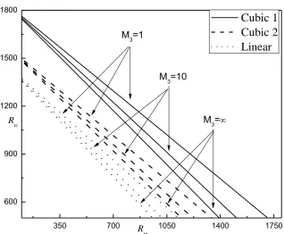
Fig. 2 shows the locus of

R

_tc and

R

_mcforvarious values of

M

₃ with three different forms of temperature profiles. In the figure, the regions over and under the curves, correspond respectively to unstable and stable ones. It is observed that there is a strong combination between

R

_tcand

R

_mcthat, an increase in the one decreases the other. This shows that, the magnetic forces becomes negligible when the buoyancy forces are predominant and vice-versa. The stability of curves are slightly bowed and in the absence of buoyancy forces (

R

_tc



0

), the instability sets in at higher values of

R

_mc indicating the system is more stable when the magnetic forces alone are present. Fig. 2 demonstrated that increasing

M

₃ has a destabilizing effect on the system. Nevertheless, this destabilization is only marginal. This may be due to the fact that a higher value of

3

M

would arise either due to a larger temperature gradient or larger pyromagnetic coefficient. Both these factors are conducive for generating a larger gradient in the Kelvin body force field, possibly promoting the instability. Besides, for a fixed value of

M

₃, the

R

_tc for cubic 1 temperature profile with

1

*

0,

2

*

0,

3

*

1

a



a



a



is shown to be the most stabilizing of all the considered types of temperature profiles, that is,

 

 

 

2 1

.

tc _linear tc _cubic tc _cubic

R



R



R

That is, the system is most unstable (i. e., augments convection) in the case of linear temperature gradient because the jump in temperature occurs nearer the less restrictive free surface, whereas the cubic1 temperature gradient makes the system more stable.

Fig. 3 shows the variations of

R

_tc and

R

_mcfor different values of heat transfer coefficient

B

_i with three different forms of temperature profiles. From the figure it is evident that an increase in the value of heat transfer coefficient

Bi

is to increase the critical Rayleigh number and hence its effect is to delay the ferroconvection. This may be due to the fact that increasing in

Bi

,

the thermal disturbances can easily dissipate into the ambient surrounding due to a better convective heat transfer coefficient at the top surface and hence higher heating is required to make the system unstable. In the figure, the

R

_tc for cubic 1 temperature profile is shown to be the most stabilizing of all the considered types of temperature profiles, that is,

 

_tc

 

_{tc 2}

 

_{tc 1}

.

linear cubic cubic

R



R



R

Hence cubic1 temperature gradient makes the system more stable and delays the onset of convection. Further in fig 4 we can observe that increase in

B

_i increases the critical wave number

a

_c and hence its effect is to contract the dimension of convection cells.

IV. CONCLUSIONS

The linear stability theory is used to investigate the result of different forms of cubic state temperature profiles on the onset ferroconvection in a ferrofluid layer. The cubic 1 temperature profile increases considerably making the system more stable compared to the other cases and are suitable for laboratory experimentation with a simulated microgravity environment. Theresult of increase in

Bi

is to setback the onset of ferroconvection, while increase in

M

₃ is to advance the onset of ferroconvection.

Table 1: Reference steady-state temperature gradients Model Reference steady-state

temperature gradient

f z

( )

a

1

*

a

2

*

a

3

*

1 Linear 1 1 0 0

2 Cubic 1

3 (

z



1)

2 _{0 0 1}

3 Cubic 2 2

Figure. 1Physical Configuration

350 700 1050 1400 1750

600 900 1200 1500 1800

R

tc

M

3

=



M

₃

=10

R

m

Cubic 1

Cubic 2

Linear

[image:6.595.139.458.304.566.2]

M

₃

=1

Figure. 2 Locus of Rtc VsRm for different values of M3 when Bi=2.

300 600 900 1200 1500 720

960 1200 1440 1680

R

_m

R

_tc

1

1

Cubic 1

Cubic 2

Linear

B

_i

=

2

1

0

2

0

2

0

Figure. 3 Variation of Rtc VsRm for different values of Bi when M3 =1.

0 300 600 900 1200 1500

2.850 2.925 3.000 3.075 3.150

a

_c

R

_m

Cubic 1

Cubic 2

Linear

B

i

=

2

1

0

2

1

2

1

0

0

REFERENCES

[1]. R. E. Rosensweig, Ferrohydrodynamics, Cambridge University Press, London, 1985.

[2]. B. A. Finlayson, “Convective instability of ferromagnetic fluids”, J of Fluid Mech., Vol 40, Mar 1970, pp 753-767.

[3]. P. J. Stiles and M. J. Kagan,“Thermoconvective instability of a ferrofluid in a strong magnetic field”, J of Colloid and InterfaceSci., Vol 134, Feb 1990, pp 435-448.

[4]. M. I. Shliomis and B. L. Smorodin,“Convective instability of magnetized ferrofluids”, J of Magn and Magn Mater., Vol 252, Nov 2002, pp 197-202.

[5]. R. Ganguly, S. Sen and I. K. Puri,“Heat transfer augmentation using a magnetic fluid under the influence of a line dipole”, J of Magn and Magn Mater., Vol 271,Apr 2004, pp 63-73.

[6]. P. N. Kaloni and J. X. Lou,“Convective instability of magnetic fluids under alternating magnetic fields”, Phys of Rev E., Vol

71, Jun 2005, pp 066311-1-12.

[7]. C. E. Nanjundappa and I. S. Shivakumara,“Effect of velocity and temperature boundary conditions on convective instability in a ferrofluid layer”, ASME J of Heat Transfer, Vol 130, Oct 2008, pp 104502-1-104502-5.

[8]. Sunil and Amit Mahajan,“A nonlinear stability analysis for magnetized ferrofluid heatedfrom below”,Proc R Soc London A, Math Phy Engg Sci., Vol 464, Jan 2008, pp 83-98.

[9]. I. S.Shivakumara, Jinho Lee and C. E. Nanjundappa,“Onset of thermogravitational convection in a ferrofluid layer with temperature dependent viscosity”, ASME J of Heat Trans., Vol 134, Jan 2012, pp 012501-1-012501-7.

[10]. C. E.Nanjundappa, I. S. Shivakumara and K. Srikumara, “On the penetrative Bénard-Marangoni convection in a ferromagnetic fluid layer”, Aerospace Science and Technology, Vol 27, Jun 2013, pp 57-66. [11]. C. E. Nanjundappa, I. S. Shivakumara, and R. Arunkumar,“Onset of Bénard- Marangoni

ferroconvection with Internal Heat Generation”, Microgravity Science and Technology, 23, 2011, 29-39. [12]. C. E. Nanjundappa, I. S. Shivakumara, and R. Arunkumar,“Onset of Marangoni- Bénard

ferroconvection with Temperature Dependent Viscosity”, Microgravity Science and Technology, 25, 2013, 103-112.

[13]. [C. E. Nanjundappa, and R. Arunkumar,“Effect of MFD viscosity on Bénard-Marangoni Ferroconvection in a rotating ferrofluid layer”, The International Journal of Engineering andScience, 07(07), 2018, 88-106.

[14]. R. Idris, and I. Hashim, “Effects of controller and cubic temperature profile ononset of Bénard– Marangoni convection in ferrofluid”, Int Commu Heat and MassTransfer, Vol 37 No 6, Jul 2010, pp 624– 628.

[15]. C. E. Nanjundappa, I. S. Shivakumara and B. Savitha, “Onset of Bénard– Marangoni ferroconvection with a convective surfaceboundary condition”: The effects of cubic temperature profile and MFD viscosity, Int Comm Heat and MassTransf, Vol. 51, Feb2014, pp 39-44.

[16]. C. E. Nanjundappa, I. S. Shivakumara, and R. Arunkumar,“Effect of CubicTemperature Profiles on ferroconvection in Brinkman Porous Medium”, Journal of AppliedFluid Mechanics, 09, 2016, 1955-1962. [17]. O. Dupont, M. Hennenberg, and J. C. Legros, “Marangoni- Bénard instabilities under non-steady

conditions. Experimental and Theoretical results”, International Journal of Heat and Mass Transfer, 35, 1992, 3237-3244.