Context estimation
in sensorimotor control
Philipp V etter
In stitu te of Neurology
University College London
All rights reserved
INFORMATION TO ALL USERS
The quality of this reproduction is dependent upon the quality of the copy submitted.
In the unlikely event that the author did not send a complete manuscript and there are missing pages, these will be noted. Also, if material had to be removed,
a note will indicate the deletion.
uest.
ProQuest U641901
Published by ProQuest LLC(2015). Copyright of the Dissertation is held by the Author.
All rights reserved.
This work is protected against unauthorized copying under Title 17, United States Code. Microform Edition © ProQuest LLC.
ProQuest LLC
789 East Eisenhower Parkway P.O. Box 1346
Abstract
Human motor behaviour is remarkably accurate and appropriate even though the
properties of our own bodies as well as the objects we interact with vary over time.
To adjust appropriately, the motor system has to estimate the context, th a t is the
properties of objects in the world and the prevailing environmental conditions. This
thesis examines how we estimate the context given th at the context is nonstationary,
it can change both deterministically and stochastically over time, and th at infor
m ation about the context, such as prior information and sensory feedback, may be
incomplete or noisy.
Psychophysical and brain imaging studies are described, showing th at to determine
the current context the central nervous system uses information from both prior
knowledge of how the context might evolve over time and from the comparison
of predicted and actual sensory feedback. A computational model is presented of
how these two sources of information are modelled and combined within the central
nervous system to derive an accurate estimate of the context th at is then used to
appropriately adjust the motor command selection.
A modelling study explores how context estimation may be used to learn and se
lect appropriate controllers within a modular architecture. The model suggests
th at prediction should precede control during motor learning and this is confirmed
psychophysically. The experimental findings are discussed with regard to their com
A cknowledgem ents
First, I would like to thank my supervisor Daniel Wolpert for guiding me into the exciting
world of psychophysics and computation with his contagious enthusiasm and rigour. Daniel
is seemingly always in a good mood, and strikes a great balance between strong support
and gentle, constructive criticism, between creative inspiration and giving me the chance
to figure a problem out for myself.
I would not have ended up in London or done a PhD in the field without the Wellcome
four year PhD programme in Neuroscience. I am greatly indebted to the committee,
Maria Fitzgerald, Alasdair Gibb, Ralf Schoepfer and primus inter pares David Attwell,
for creating such a rich à la carte PhD and for providing a safety net should anything go
wrong. I would like to thank Zoubin Ghahramani, my second supervisor, for conveying his
expertise on all things mathematical in such an intuitive way. I would also like to thank
Randy Flanagan for stimulating discussions, besides being a great squash coach. Further, I
am grateful to Mitsuo Kawato for giving me the opportunity to spend two intensive weeks
in Kyoto, working together with Jan Peters.
My PhD was strongly infiuenced by my context — the people in the Wolpert-lab and the
Sob ell Department, administrative and scientific, who made this a fun three years. In
particular, I would like to thank Pierre Baraduc, Susan Goodbody, Antonia Hamilton and
Alexander Korenberg for their support in many different guises — from reading this thesis
to bringing me back down to earth when my attempts at philosophising got out of hand.
Finally, I would like to thank my web of friends and my family, who ensured a productive
Collaborations
I would like to express my thanks to Daniel Wolpert, who worked with me on all
projects, as well as my collaborators on individual chapters: Susan Goodbody in
Chapter 2, Bal Athwal, Richard Passingham and Richard Frackowiak in Chapter 5,
Zoubin Ghahramani in Chapter 6 and Randy Flanagan in Chapter 7. I was lead
investigator on all projects in this thesis, except for Chapter 5, where I was co-lead
investigator with Bal Athwal.
The work in Chapters 2, 3 & 4 resulted in three publications
• P. Vetter, S. Goodbody and D.M. Wolpert (1999). Evidence for an eye-centred
spherical representation of the visuomotor map. J. Neurophysiol 81:935-9
• P. Vetter and D.M. Wolpert (2000). Context estimation for sensorimotor con
trol. J. Neurophysiol <9^:1026-34
• P. Vetter and D.M. Wolpert (2000). The CNS updates its context estimate in
C ontents
Abstract 2
Acknowledgem ents 3
Collaborations 4
C ontents 5
1 Introduction 14
1.1 Problems of context e s t i m a t i o n ... 14
1.1.1 Coordinate tra n s fo rm a tio n s ... 15
1.1.2 Sensory feedback delays ... 15
1.1.4 N o n sta tio n a rity ... 18
1.1.5 A computational fra m e w o rk ... 19
1.2 Coordinate transformations ... 21
1.2.1 Visuomotor m a p ... 21
1.2.2 Function approximation p ersp ectiv e... 22
1.2.3 Neurophysiology ... 23
1.3 Noise and e s tim a tio n ... 24
1.3.1 Estim ating static s ig n a ls ... 24
1.3.2 Estimating time-varying s ig n a ls ...25
1.3.3 Neurophysiology of e s tim a tio n ...27
1.4 Modularity for c o n t r o l ... 28
1.4.1 Multiple task l e a r n i n g ... 29
1.4.2 Modular control a rc h ite c tu re s ... 31
1.4.3 Cerebellum and modular co n tro l... 35
1.5 Summary of experimental c h a p t e r s ... 39
2 Generalisation o f the visuomotor transformation 40 2.1 A b s tr a c t... 40
2.2 In tro d u c tio n ...41
2.3 M e th o d s ... 42
2.4 R e s u lts ... 47
3 C ontext estim ation with feedback 53
3.1 A b s t r a c t ... 53
3.2 In tro d u c tio n ... 54
3.3 M e th o d s ... 55
3.4 R e s u lts ... 61
3.5 D isc u ssio n ... 69
4 Context estim ation without feedback 75 4.1 A bstract ... 75
4.2 In tro d u c tio n ... 75
4.3 Methods ... 78
4.4 R e s u lts ... 82
4.5 Discussion ... 85
5 Imaging uncertainty and inconsistency in context estim ation 90 5.1 A b s t r a c t ...90
5.2 In tro d u c tio n ... 91
5.3 M e th o d s ... 93
5.4 R e s u lts ... 97
6 Context estim ation for modular control 106
6.1 A b s t r a c t ... 106
6.2 In tro d u c tio n ... 107
6.3 M o d e l ... 112
6.4 R e s u lts ... 115
6.5 D isc u ssio n ... 125
6.6 Appendix: Learning ... 128
6.7 Appendix: Arm d y n a m ic s ... 129
7 Motor learning of prediction versus control 131 7.1 A b s t r a c t ...131
7.2 In tro d u c tio n ... 132
7.3 M e th o d s ...134
7.4 Results ...136
7.5 D isc u ssio n ...143
8 General discussion and conclusions 147 8.1 A b s t r a c t ... 147
8.2 Summary ... 147
8.3 Emerging q u e s tio n s ... 151
8.3.2 Relating context estimation and forward-inverse models . . . .1 5 3
8.3.3 Context estimation beyond motor c o n tro l...154
8.3.4 Time scales of estim atio n ...156
8.3.5 Granularity of modular a rc h ite c tu re s ... 158
8.4 Context estimation and neural s tr u c tu r e s ...159
8.4.1 W hat is the c o n te x t? ... 160
8.4.2 Representation of internal s t a t e ... 160
8.4.3 Representation of goal-relevant v a r ia b le s ... 163
8.5 C o n c lu sio n s ...165
List o f Figures
1.1 Simplified scheme of context e s tim a tio n ...20
1.2 Cerebellar c ir c u itr y ... 36
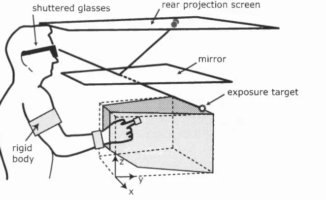
2.1 Virtual reality setup ...44
2.2 Change between pre- and post-exposure pointing ... 48
2.3 Change in pointing with distance from exposure t a r g e t ...50
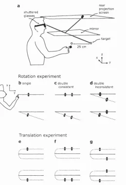
3.1 Apparatus and pointing p a ra d ig m ... 57
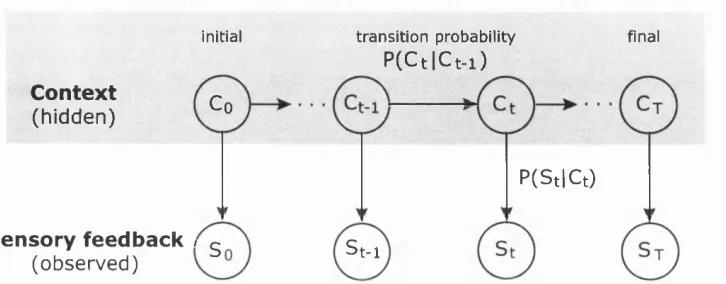
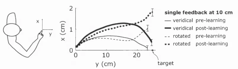
3.2 Context evolution with sensory feedback as a hidden Markov process 60 3.3 Finger paths before and after learn in g ... 62
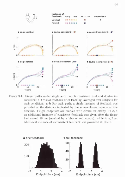
3.4 Finger paths under different feedback c o n d itio n s ...64
3.5 Distribution of endpoints in post-learning t r i a l s ...64
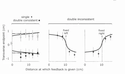
3.7 Translation experiment: Transverse endpoints as a function of feedback 67
3.8 Translation experiment: Transverse pointing positions relative to the
time of feedback... 67
3.9 Simulation of context estimation during a movement ... 72
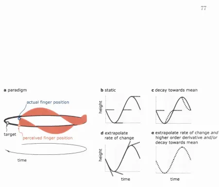
4.1 Paradigm and model p redictions... 77
4.2 Schematic of two context estimation s tr a te g ie s ... 83
4.3 Tracking perform ance... 84
4.4 Tracking performance in the second e x p e r im e n t... 86
5.1 Context estimation paradigm ... 95
5.2 Brain activation under uncertainty with online feedback... 100
5.3 Brain activation in inconsistent gain trials compared to normal gain trials...101
6.1 Schematic of MOSAIC a r c h ite c tu re ... 112
6.2 MOSAIC learns multiple linear m ap p in g s... 116
6.3 Schematic of nonlinear input e x p a n sio n ...118
6.4 Nonlinear MOSAIC performance on multiple nonlinear mappings . . 119
6.5 MOSAIC learns a nonlinear m a p p in g ... 120
6.6 MOSAIC performance on 2 joint arm with different numbers of modules 123 6.7 Velocity profiles in eight movement directions ...123
7.1 Kinematic l e a r n i n g ... 137
7.2 Grip and load force profiles development over learn in g ...139
7.3 Replication of initial t r i a l s ... 141
7.4 Comparison of kinematic and grip le a rn in g ...142
List o f Tables
2.1 Mean prediction errors for individual subjects and hypotheses . . . . 50
5.1 Brain activity m o v e m e n t-re s t... 98
5.2 Brain activity feedback-no feedback...99
5.3 Brain activity in interaction between no prior information and feedback 99
5.4 Brain activity in inconsistent minus consistent t r i a l s ...100
1 Introduction
Hum ans easily generate skilled and accurate m ovem ents that are far more com plex than the m ost advanced robots of today. The task that is being solved in doing this is to generate appropriate m otor commands in order to achieve desired consequences. The main them e of this thesis is that appropriate m otor commands are adjusted according to the prevailing m ovem ent context^ which em bodies parameters of both our own m otor system and the outside world. Using psychophysical, m odelling and func tional brain im aging approaches this thesis explores how the CNS may estim ate the context and subsequently use it for control.
1.1
Problems of context estimation
Our ability to generate accurate and appropriate motor behaviour is based on ad
justing our motor commands to the prevailing movement context. This context
embodies param eters of both our own motor system, such as the level of muscle
fatigue, and the outside world, such as the weight of a bottle to be lifted. As the
consequence of a given motor command depends on the current context, the central
nervous system (CNS) has to take the context into account to achieve accurate con
it can only gain information about it through sensory feedback. Sensory feedback
is not equivalent to the true context, but it can be processed in order to obtain an
estim ate of the true context. This estimation process is non-trivial because of four
m ain issues:
1. coordinate transformations
2. sensory feedback delays
3. sensory noise
4. nonstationarity
I will now describe these problems in turn.
1.1.1
Coordinate transformations
Receiving visual sensory feedback about a target, does not immediately tell our
m otor system how to reach the target. The visually (or otherwise) defined target
location has to be transformed into coordinates appropriate for movement. Coordi
nate transform ations are not just necessary from visual to motor coordinates, but
also from auditory and tactile sensory inputs. Further, sensory information from
multiple modalities often has to be integrated. Chapter 2 investigates the represen
tation of the visuomotor transformation. The m athem atical tools used to describe
coordinate transformations as well as some neurophysiological findings pertaining
to the visuomotor transformation are introduced in Section 1.2.
1.1.2
Sensory feedback delays
The feedback from our sensors has time delays th at are significant compared to the
duration of a movement. The requirement and ability of our motor system to com
estim ate might become quite inaccurate if the estimation process does not compen
sate for the feedback delays. For instance, visuomotor delays are on the order of a
quarter of a second — a sprinter covers 2.5 m in th at time. Such long sensory feed
back delays may be overcome by a mechanism th at continually predicts one quarter
of a second into the future, to provide an estimate of the current context. There
is ample experimental evidence for the existence of such predictive mechanisms,
for instance when one body part acts on another (Massion 1992; Lacquaniti 1992;
Nashner 1982; Gahery and Massion 1981), during self-produced removal of a load
in the other hand (Dufosse et al. 1985; Lum et al. 1992), ball catching (Lacquaniti
1996; Lacquaniti and Maioli 1987; Lacquaniti and Maioli 1989) and other postural
adjustments (Bouisset and Z attara 1987; Gordo and Nasher 1982; Lee et al. 1987).
One idea th at has been very im portant in this research is the notion of internal
forward models. Internal models are neural systems th at simulate the behaviour
of natural processes and in so doing transform sensory signals to motor commands
and vice-versa. There are two types of internal models, known as forward and in
verse models (Jordan 1995; Miall and Wolpert 1996; Wolpert 1997; Wolpert and
Ghahramani 2000). The forward model is a causal representation of the motor ap
paratus th at represents the behaviour of the motor system in response to outgoing
motor commands (Kawato et al. 1987; Jordan and Rum elhart 1992; Miall and
Wolpert 1996; Wolpert et al. 1995). T hat is, forward models capture the causal
relationship between actions and outcome. Forward models are also known as pre
dictors. Inverse models capture the transformation from desired consequences to
motor outputs. Unlike forward models, the inverse model is not necessarily unique
as the transformation can be one-to-many. Fast feedforward control can be achieved
through an inverse model of the controlled object, and therefore, an accurate inverse
model could act as an ideal feedforward controller. For this reason, inverse models
are sometimes called (feedforward) controllers.
One of the uses of forward models in motor control is to compensate for time delays
feedback, simulating the system dynamics in neural hardware could eliminate this
time delay (Miall et al. 1993; Miall and Wolpert 1995). The use of forward models
to compensate for feedback delays has been studied intensively, and does not form
a focus in this thesis.
1.1.3
Sensory noise
Even though forward models may compensate for feedback delays, the sensors from
which sensory feedback originated are noisy, and often provide incomplete informa
tion about the context. We have no visual feedback for instance, if we close our
eyes, or perform a task outside our visual field.
In order to generate accurate movements, the CNS has to deal with both sensory
and motor noise. By noise I mean th at our sensors do not provide us with infinitely
accurate information, and our muscles do not generate forces with infinite precision.
Sensory variability can be split into a bias component, which is the difference be
tween the actual value and the average sensor-measured value of a parameter, and a
variance component describing the spread of the measurements around the average.
In this thesis I focus on the variance (or the related standard deviation), th a t is the
noise.
Visual direction acuity has a standard deviation of 0.2-0.6° (Hansen and Skavenski
1977). The standard deviation of proprioceptive accuracy has been estim ated at
0.5-0.7° at a joint based on physiological data (Scott and Loeb 1994), similar to
psychophysical measurements of 0.6-1.1° in position matching experiments (van
Beers et al. 1998). Interestingly though, if the task is to explicitly assume particular
joint angles, the measured accuracy decreases to 1.3-3° (Clark et al. 1995). Our
motor output is noisy too, with the standard deviation for a constant force at about
1% of the required force level (Slifkin and Newell 1999) and around 10% for a force
pulse (Schmidt et al. 1979).
estim ated mathematically. Chapter 3 applies one of these frameworks to sensori
m otor context estimation, in order to explain results obtained from psychophysical
pointing experiments.
1.1.4
Nonstationarity
Finally, the context is not static but tends to evolve in a structured, but often
uncertain way. For example the weight of a bottle tends to decrease as we pour
from it, and muscles fatigue with use. More dramatically, the dynamics of our body
change abruptly, as soon as we pick up an object and manipulate it, such as when
using a tennis racket. The property th at the context can change — smoothly or
discretely — over time is referred to as nonstationarity. Section 1.3 provides a com
putational perspective on how to characterise this nonstationarity, while Chapters 3
& 4 explore, in psychophysical pointing paradigms, how the movement context is
estim ated under nonstationarity.
As the context changes, the associated control problem changes too. There are two
distinct strategies to solving this control problem. One is to use a single, sophis
ticated controller, th a t will rapidly adapt to the current context. However, such
a controller would be enormously complex to allow for all possible scenarios. If
this controller were unable to encapsulate all the possible contexts, it would need
to adapt every time the context of the movement changed before it could produce
appropriate motor commands — this would produce transient and possibly large
performance errors. Alternatively, a modular approach (reviewed in Section 1.4)
can be used in which multiple controllers co-exist, with each controller suitable for a
small set of contexts. Using this approach, there is an additional need for a process
which selects the appropriate controllers at the right time.
Studies of motor adaptation have suggested th at we are able to learn multiple con
trollers and switch between them based on context. Adaptation to visuomotor or
and on a time scale th a t can extend to hours. However, on removal of the per
turbation, de-adaptation is usually very rapid. These results can be interpreted as
representing learning of a new controller in the former case, and switching back to
a stably learned module in the other. In support of this notion, subjects adapt
increasingly rapidly to repeated presentations of kinematic (McGonigle and Flook
1978; Welch et al. 1993) or dynamic perturbations (Brashers-Krug et al. 1996).
Beyond the experimental evidence for modularity in motor control, there are also
com putational benefits to using a modular approach. First, the world itself is mod
ular, in the sense th a t we interact with many different objects and environments.
A modular approach could take advantage of this structural feature of the world.
Secondly, modular learning implies th a t learning one module need not interfere with
other modules. The lack of cross-talk could result in faster learning and better re
tention of previously learned modules. Finally, since many novel contexts are in
fact combinations of previously experienced elements of the context, it should be
easy with a modular approach to generate appropriate behaviour for new combina
tions of previously learned contexts. Chapter 6 examines a novel modular control
architecture, MOSAIC, in particular, whether it is able to partition dynamics.
1.1.5
A computational framework
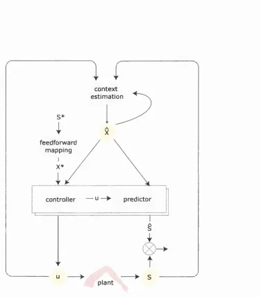
Figure 1.1.5 shows a computational framework within which all experiments in this
thesis can be related to each other. This figure will be referred to throughout the
thesis. For any goal-directed movement, such as picking up an apple, the goal may
initially be defined visually in retinal coordinates S*, where the * denotes a desired
state. This then has to be transformed or mapped (feed-forward mapping) into
coordinates appropriate for moving the arm X*. Chapter 2 looks at the learning and
representation of this transformation, while its neurophysiological and mathem atical
basis is introduced in Section 1.2. This transformation depends on a good estimate
of where the arm is at present, it’s context estimate X , where ^ means estimate. I
context estimation S *
X feedforward
mapping X *
controller — u predictor
/ \
> S
u
plant
environment th at are required to perform the task. Context estim ation is non-trivial,
because sensory information, may be noisy or missing. Chapter 3 introduces a model
of the relationship between sensory feedback and the true context, and explores
how sensory feedback may be used to update the current estim ate (5 —>-context
estimation). Chapter 4 examines how the estimate is updated in the absence of
sensory information.
Accurate context estimation is a prerequisite for accurate movement. The final step,
movement generation, is achieved through a controller, which takes information of
the desired configuration, and the current context estimate X to generate a motor
command u. As outlined in the previous section, it may be a powerful strategy to
solve the control problem arising from the nonstationarity of the context using a
m odular approach, th at is using many different controllers. W ith regard to this.
C hapter 6 examines MOSAIC, a novel modular architecture. Section 1.4 reviews
properties of different modular control architectures.
1.2
Coordinate transformations
1.2.1 Visuomotor map
The human CNS receives sensory inputs from different modalities which are initially
represented in disparate coordinate systems. In action, coordinate transform ations
are used to convert sensory information into coordinates appropriate for movement.
For example, when reaching to a visually perceived target in space, the target loca
tion in visual coordinates must be converted into a representation appropriate for
movement, such as the target posture of the arm. The coordinate transform ation
between the visual location of the arm to the configuration required to place the
hand at th at location is known as the visuomotor map. The visuomotor map can
adapt to changes of the relationship between visual and motor coordinates, as they
and Stratton (1897,1897a) first studied this relationship systematically, by examin
ing the change in visuomotor coordination under prismatically induced displacement
and rotation. Subsequently, many studies have further demonstrated the ability of
the visuomotor map to adapt, at least partially, to a wide variety of alterations in
the relationship between visual and motor system (Welch 1986).
1.2.2
Function approximation perspective
The problem of learning the relationship between visual coordinates (input) and co
ordinates appropriate for movement (output), can be regarded as a function approx
imation problem (Pouget and Snyder 2000). The mathematical theory of function
approximation is concerned with estimating a function from samples of input-output
pairs. At one extreme, a function approximator can be represented as a look-up ta
ble in which corresponding input-output pairs are stored (Atkeson 1989; Rosenbaum
et al. 1993). Thus, the visuomotor coordinate transformation could be represented
as a set of pairs of visual and motor coordinates. At the other extreme of the spec
trum , a coordinate transformation can be represented as a model parameterised by
the physical attributes of the transformation. Thus, the motor coordinates can be
represented as function of the visual coordinates parameterised by the felt configu
ration of the eyes, head and arm.
Intermediate between local and global models are (radial) basis function networks
(Broomhead and Lowe 1988). These networks approximate the function via a su
perposition of bases, for instance Gaussian receptive fields, and can be derived by
assuming th at the function approximator trades off the closeness of fit to the input-
output data and the smoothness of the resulting function. (A lookup table is less
smooth than a global parameterisation.) The number of parameters required in this
representation is intermediate between local and global. The representation of the
1.2.3
Neurophysiology
The process of relating a visual target location as it appears on the retina to the
sequence of muscle activations to reach it is known as the visuomotor map. A
key effect of altering this process, is th at the correspondence between visual and
proprioceptive input has to be modified or recalibrated. In looking for a neural
substrate for this correspondence region, it is interesting to note th at posterior
parietal cortex shows an increase in regional cerebral blood flow in position emission
tomography (PET) when participants adapt while wearing prism glasses (Glower
et al. 1996).
This fits well with single cell recordings in the ventral intraparietal area of the
monkey parietal cortex, where cells have bimodal receptive fields. This means th at
they respond to proprioceptive input at a certain location on the body (for instance
the hand) with the same firing pattern as when a visual stimulus is close to th at
location (Colby et al. 1993; Baizer et al. 1991; Colby and Duhamel 1996). These
receptive fields are highly plastic. For instance, when holding a tool, the bimodal
receptive field of the hand may transfer to the end of the tool (Iriki et al. 1996).
Very similarly — mirrored across the principal sulcus — premotor neurons in area
F4 also have bimodal receptive fields (Fogassi et al. 1996; K urata and Tanji 1986).
The visual-proprioceptive congruence is not the only target when modifying the
relationship between target position and sequence of muscle activations to get there.
Many other brain areas involved in the parietofrontal network are involved (for a
review see Battaglia-Mayer et al. 1998; Wise et al. 1997). This greater network
processes additional information about eye position, gaze orientation and retinal
information. As it is highly interconnected, it is unsurprising th at many areas are
1.3
Noise and estimation
1.3.1
Estimating static signals
Sensory psychophysics
In classical psychophysics sensory noise is not measured directly, but inferred from
the subject’s ability to discriminate two stimuli. In the simplest case, the stimulus
is static. Weber’s law states th at the just noticeable difference A S between two
stimuli (and thus also the noise) scales with the magnitude of the stimulus 5 , such
th a t ^ is constant (Weber 1846). For most sensory systems the noise is assumed to
be Gaussian. Under this noise distribution and for a static stimulus, the tem poral
average of the sensor measurements is an optimal estimate of the stimulus assuming
a squared error cost function (Bishop 1995).
Bayes’ rule
There is no principled way to improve on the temporal average if no additional
information about the signal is available. However, if we have a prior expectation
or model M of what the signal S should be, then the estimate can be improved
on (provided the prior expectation is not completely useless). The reverend and
m athem atician Thomas Bayes (1702-1761) formalised how to update P{ M ), the
probability distribution of the prior expectation M, in the face of sensory feedback
S. Bayes’ rule states th at the posterior probability distribution of the signal, in
other words the improved model of the true sensory feedback P {M \S ) =
where P{S \M ) is the likelihood, the probability distribution of the sensory feedback
S given the true signal is M; P{M) is the probability distribution of the prior
expectation M and P (5 ), a normalising term known as evidence, is the probability
As an example, we may know a priori th at when wearing a particular pair of goggles
we are either going to receive right-rotated feedback P [ Mr) = 0.9 or left-rotated
feedback P { Ml) = 0.1 and after initiating an arm movement towards a target,
visual sensory feedback S is obtained. It may be the case th at the likelihood of
S under right-rotated feedback Mr, P { S \ Mr), is 0.3, while the likelihood of left-
rotated feedback Ml is P { S \Ml) = 0.2. Using Bayes’ rule, the posterior probability
of the context being right-rotated feedback is
If we have no prior expectation, in other words the distribution P {M ) is flat, then the
calculated posterior P{ M \S ) is proportional to the likelihood distribution P{S \M).
Since sensory noise is assumed to be white, the likelihood distribution is Gaussian.
Thus the best single estimate is then the maximum likelihood value. If, however,
there is a prior expectation, then the posterior distribution may differ from the
likelihood distribution, and Bayes’ rule cannot be short-cut. In practise, only the
maximum of the posterior distribution is usually calculated.
1.3.2
Estimating time-varying signals
Often the signal we are interested in, for instance a moving target, changes over time.
One option is to simply apply Bayes’ rule iteratively at each time step. However, this
approach intrinsically biases the results to remain similar. A better time-varying
estimate can be made if we can formalise our knowledge about the tem poral structure
in the system, for instance by using a hidden Markov process or a Kalman Filter.
Hidden Markov processes
In the simplest case of a hidden Markov process, the system is only in one of two
it switches. Furthermore, the probability of switching only depends on the current
state. In the general case, the system may be in one of n discrete states, where the
probability distributions of transitioning from one of the n states to any of the n
states, describe the dynamics of the system over time. This is known as a Markov
process, which is first order, because the transitions only depend on the current
state, not on previous states. However, in many cases the state cannot be measured
directly, but has to be inferred from noisy sensory feedback, which is termed a hidden
Markov process (Rabiner and Juang 1986; Baum et al. 1970). Assuming th a t the
system dynamics are Markovian, two problems have to be solved. First, the number
of states and the transition probabilities have to be determined, which is also known
as system identification or learning. Second, given the model parameters and a time
series of sensory feedback we have to determine the underlying states, in a process
called inference (for a review see Roweis and Ghahramani 1999). Interestingly, the
state sequence formed by taking the most probable state of the posterior distribution
at each time is not necessarily the single state sequence most likely to have produced
the observed data.
Kalman filter
Instead of assuming a discrete state, the Kalman filter has continuous states th a t
are updating deterministically but with process noise, for example Xt+\ = A X t + Wt
where Xt is the state of the system (a vector), A is the state transition m atrix
and w is white process noise. In analogy to hidden Markov processes, the state
is only observable indirectly through noisy sensory feedback Yt = C X t + Vt where
Y is the sensory feedback, C the output m atrix and v white sensory noise. The
process takes its name from Kalman, who derived an efficient recursive optimal
solution to the inference problem (Kalman 1960; Kalman and Bucy 1961). This
recursive formulation uses a so-called Kalman gain which weighs the state estim ated
based on sensory feedback, with the state estimate based on the previous state.
th a t is determined by the relative magnitudes of the process and sensory noise. For
instance, in an arm movement study, subject’s arm position estimates were modelled
as a Kalman filter whose Kalman gain asymptotes after about one second (Wolpert
et al. 1995).
Extended Kalman filter
The classic Kalman filter assumes the dynamics of the system to be linear. However,
the dependence on the previous state may be nonlinear, such th a t Xt+i = f(Xt)+Wt.
To make this system tractable, the trick is to calculate the current state m atrix At
by linearising / around the current state Xt, At = - ^ \ x f This powerful extension
to the Kalman filter is widely used in engineering.
Comparisons
The power of the Kalman filter is th at it works with continuous states, while the state
transitions are limited by the linear state m atrix A. The hidden Markov process,
in contrast can implement nonlinear dynamics through appropriate state transition
matrices, but it is limited by the fact th at there are only a limited number of discrete
states. The m athem atical tools of system dynamics just reviewed may serve as useful
descriptions of how the true context evolves, and also of how the CNS estimates the
context. Chapter 3 uses a hidden Markov model of how the CNS estimates the
current context to quantitatively fit psychophysical pointing data.
1.3.3
Neurophysiology of estimation
State estimates can be generated by integrating the result of multisensory integra
tion (e.g. visuo-proprioceptive congruence) with the output of a sensory prediction
model. As discussed in Section 1.1.5, the operational definition of the context en
periphery, such as desensitisation, can be interpreted as operations towards esti
m ating the context. However, here the focus is on higher-level brain areas th a t are
responsible for providing other brain areas with the information of where the hand
or an object it is controlling is.
A recent study described a patient whose context estimation was impaired after
damage to the superior parietal lobule (Wolpert et al. 1998). Dramatically, this
patient would ‘forget’ th at she was holding a cup if she did not attend to it, leading
to her dropping it. Pisella et al. found evidence for an ‘autom atic pilot’ relying
on spatial vision which drives fast corrective arm movements th a t can escape inten
tional control (Pisella et al. 2000). This phenomenon was absent in a patient with a
bilateral lesion of posterior parietal cortex. Desmurget et al. derived similar conclu
sions from an experiment in which subjects made fast corrective arm movements to
target jum ps th a t were suppressed when the posterior parietal cortex was subjected
to transcranial magnetic stimulation (TMS) at movement onset (Desmurget et al.
1999).
These findings have analogues in the primate literature, where Eskandar and As
sad (1999) found cells in the lateral intraparietal area th at could be interpreted as
predictive signals of where visual feedback should be. Other studies have found
cells in areas V6a / 7m (Obayashi et al. 2000) and — homologously in premotor
area 6 (Graziano 1999) — th at ‘predict’ hand location by being active during hand
movement, regardless of whether the hand is visible.
1.4
Modularity for control
M odularity can be explored experimentally through learning paradigms, since once
performance asymptotes it is difficult to assess how this performance comes about.
Alternatively, m odularity can be explored theoretically by analysing the behaviour
of different m odular architectures. In general there are two critical issues: first,
a single task solution is itself represented modularly, in the form of smaller building
blocks or primitives. Chapter 6 examines in simulations, whether multiple solutions
for the same task under different contexts can be learned by a particular modular
control architecture. Learning multiple solutions for the same task is an extreme
form of nonstationarity, in which the context can change abruptly.
1.4.1
Multiple task learning
In multiple task learning experiments, it is useful to distinguish between two types of
tasks, ones in which new relationships between perceived and actual spatial locations
are learned (kinematic mappings), and tasks in which new relationships between a
given movement and the forces necessary to generate it have to be learned (dynamic
mappings).
Modular learning explores whether it is possible to learn two different mappings in
parallel. If this is the case, then the next question is, how easy it is to switch from
one to another mapping. Finally, it would be interesting if the appropriate mapping
could be pre-cued. Interestingly, in perception a neural analogue for such state-
dependent learning has been demonstrated. When rat whiskers were stim ulated
together with the application of acetylcholine, this resulted in long-lasting response
modifications, the recall of such altered responses depended on the presence of ex
ogenous acetylcholine (Shulz et al. 2000).
Kinematic learning is classically explored by wearing prism glasses which alter the
relationship between a viewed location and the associated arm posture to reach it.
The question is, whether one can be pre-cued to ‘know’ which mapping is needed
for the different prisms worn. Most learning paradigms involve two mappings such
as from left-displacing and right-displacing prisms. Learning can be measured by
analysing the extent to which subjects adapt to the new mapping. A more direct
measure is to remove the new mapping and observe the after-effect of having been
Previous studies have shown th at the motor system can, at least partially, adapt to
m ultiple prisms (Kravitz and Yaffe 1972; Welch et al. 1993) and is able to select the
appropriate behaviour when the context is cued by gaze direction (Kohler 1950; Hay
and Pick 1966; Shelhamer et al. 1991), body orientation (Baker et al. 1987), arm
configuration (Gandolfo et al. 1996) or an auditory tone (Kravitz and YafFe 1972).
The contextual cue can also be given through a visual scene which creates illusory
self-rotation (Cohn et al. 2000). When the cue given is intermediate between two
cues each associated with a different context, the behaviour seen is consistent with
mixing of the learned behaviours (Ghahramani and Wolpert 1997).
C hapter 3 explores an area th at has received less attention, namely how within-
movement information can be used to select the appropriate mapping. Most previous
within-movement studies have focused on how sensory feedback is used within a
single context to improve accuracy (Elliott et al. 1995).
Dynamic learning experiments have shown th at subjects can learn to compensate
for force fields th a t are deterministic functions of the velocity and/or position of the
hand (Shadmehr and Mussa-Ivaldi 1994), but not explicitly functions of time (Con-
d itt and Mussa-Ivaldi 1999). These experiments typically involve making planar 10
cm reaches in several directions from a starting location. There is still some debate
as to how these force fields are learned (Shadmehr and Mussa-Ivaldi 1994; Con-
d itt et al. 1997; Thoroughman and Shadmehr 2000). Chapter 4 examines whether
explicitly time-varying kinematic perturbations can be learned.
Brashers-Krug et al. (1996) showed th at learning a clockwise viscous curl field
interfered dramatically with the learning of an anti-clockwise curl field immediately
afterwards. This interference disappeared if the learning periods were separated by
more than 6 hours. Functional brain imaging revealed a shift in activation from prefrontal regions of the cortex to the premotor, posterior parietal and cerebellar
cortex structures during the consolidation period (Shadmehr and Holcomb 1997). It
is possible to cue two opposite curl fields by using different hand postures to hold the
coloured light (Gandolfo et al. 1996).
Recently, Krakauer et al. (1999) found th at learning novel kinematics is indepen
dent of learning novel dynamics, by showing th a t there is no interference between
learning novel kinematics K and dynamics D. Flanagan et al. (1999) used a slightly
different approach to come to a similar conclusion: they showed th a t performance on
the combination K+D was improved by learning K and D separately. Conversely,
learning the combination K+D improved subsequent performance of K alone (but
not D).
1.4.2
Modular control architectures
Our ability to coordinate movement testifies to the quality of control we have over
our nonlinear and nonstationary dynamics. This task might be solved by using a
divide and conquer strategy in which a complex problem is somehow partitioned
into a number of simpler sub-problems th at can be solved independently, and whose
individual solutions yield the solution of the original complex problem.
The divide and conquer strategy raises several questions. How is the problem de
composed? How many sub-problems are there? How does each model know which
sub-problem it is responsible for? W hat and when does each model learn? Is each
model exclusively responsible for one sub-problem? How complex is an individual
model? Are all models structurally equivalent?
Interestingly, the answers to these questions in control theory, neural networks,
statistics, artificial intelligence and fuzzy logic are similar, although the nomen
clature is diverse, calling them local model networks (Johansen and Foss 1992; Jo
hansen and Foss 1993), operating regime-based models (Johansen and Murray-Smith
1997), multiple model estimation and adaptive control (Saridis and Dao 1972; Sten
gel 1986), gain scheduled controllers (Rugh 1991), heterogeneous control (B. and
(Opoit-sev 1970; Kasavin 1972), local regression techniques (Schaal and Atkeson 1998) or
Takagi-Sugeno fuzzy models (Takagi and Sugeno 1985).
D ecom position
Several approaches to the problem of decomposition have been proposed. One way
in which to do this is to partition the problem according to the physical components,
such as the hand, arm and trunk. This partitioning has the advantage of locally
decreasing the degrees of freedom of each controller. However, control will be poor
if there are strong interactions between components (interaction torques are non-
negligible (Bastian et al. 1996; Gribble and Ostry 1999)). Alternatively, the task
may be decomposed according to phenomena, for instance by asking whether the
movement in question is rhythmic or not. A further possibility is to divide up
complexity according to different goals. For instance, there may be one module for
playing tennis, and another for writing (Wolpert and Kawato 1998). Finally, the
complexity may be partitioned according to the nonlinearity of the system dynamics.
For instance, there might be one model for the arm, when the interaction torques
are negligible, and a different one for an operating range in which the nonlinear
interaction torques do become significant. This last approach is widely used in
engineering. Research has recently focused on finding implementations of such an
architecture which learn to self-partition.
The answer to the identification problem of how many sub-problems there are is
either to fix the number of modules, or, using a constructive approach (Narendra
et al. 1995; Narendra and Balakrishnan 1997; Schaal et al. 2000), to add a new
model, every time system performance drops below a threshold. Since neurons are
post-mitotic (with a few exceptions, see for instance Horner and Gage 2000), having
Selection
Modular approaches invariably require a gating mechanism to select the right model.
The gating mechanism is the feature which differs most strongly between architec
tures. One option is to formulate a set of rules (‘if holding a tennis racket then use
the tennis model’) and to base selection on that. If such rules encompass a number
of conditional statem ents like in a flowchart, then this procedure can be formulated
as a hierarchical decision tree (Breiman et al. 1984; Friedman and Roosen 1995).
Taking decisions based on a decision tree is very easy. Learning the optimal decision
tree in the first place, however, is more difficult. Given a decision question such as
‘is the object in my hand heavier than x g?’ there are in general two criteria to
find the optimal value of x. In classification trees such as CART [Classification
And Regression Trees] the criterion is to minimise the probability of choosing the
wrong model, hence ‘classification’. Alternatively, regression trees such as MARS
[Multiple Adaptive Regression Splines], use a squared error criterion between desired
and actual output to minimise the output error of the tree. In other words, it is not
the identity of the model selected th at is im portant, but the output of the selected
model. In MARS, the output of each model is a particular linear regression of the
input vector.
One problem with standard decision trees is th at decisions are discrete, and when
switching from one model to the next there may be discontinuities in control.
Smooth transitions between models occur naturally, however, if decisions in a deci
sion tree are made according to fuzzy logic.^
Alternatively, smoothness can be achieved using probabilistic models such as Jor
dan and Jacobs’ (hierarchical) mixture of experts (Jacobs et al. 1991; Jordan and
Jacobs 1994)^. Here, each model i ‘answers’ the decision tree questions separately.
while a gating network then combines these answers to an overall answer. For each
model a gating value n* can be calculated, which is a linear regression of the input^.
The probabilistic element in the architecture is to not simply select the model with
the biggest gating value u, which would be a winner-takes-all situation. Rather, the
overall answer is the responsibility-weighted sum of all answers, where the respon
sibility of each model is the softmax-normalised gating value
MOSAIC is another architecture which also uses the softmax transform as a proba
bilistic element. In contrast with the mixture of experts, however, the gating value is
not calculated by an input-dependent gating network. Instead, the mixture of (con
trol) models is augmented with their own predictors, which try to predict the sensory
consequences of control (Wolpert and Kawato 1998). The softmax-normalised pre
diction errors — which depend on the output of the system — are used as gating
values to select the appropriate control models.
Learning
In neuroscience, it is not clear how prior knowledge may be available to partition the
models, and thus current modelling methods concentrate on autom atic partitioning
procedures. Automatic partitioning procedures assign a given model responsibility
during control. To learn the right responsibilities, one could let each model give its
output in turn and then pick the one th at is best. However, this would provide the
information too late. One option in this case is to store when each model is most
appropriate. Classically, what one can do is to take im portant regions in the state
space, train one model there and then go to the next region. Here the time when
each model has to learn is given from the outside. To self-supervise learning a trick
is to associate each controller with a predictor th a t predicts what is going to happen.
logic is deemed ’orthogonal to probability theory as it focuses on ambiguities in describing events, rather than uncertainty of occurrence or non-occurrence’(Pearl 1988), but it is possible to describe fuzzy logic in terms of uncertainty of which label to use. In the multiple model case a fuzzy representation of model selection would amount to uncertainty about which local model was the correct one for a given non-fuzzy operating point.
The controller associated with the predictor th at generates the best prediction, then
receives the biggest share in controlling (Wolpert and Kawato 1998).
Model complexity
Modular architectures can be made arbitrarily accurate either by increasing the
number of models, or by making the local models sufficiently complex. In the
upper limit of single model complexity, there is one global model, at the other end
the architecture is a lookup table. A classical multilayer perceptron network is
intermediate on this scale, while decision trees generally have simple models.
How complex, therefore, should an individual model be? In engineering, by default
models are assumed to be linear. Both simpler, locally constant models as well
as more complex polynomial models have been explored (Pottm ann et al. 1993).
Even more powerful multilayer perceptron models can learn any smooth relationship
(Rumelhart et al. 1986). In general, a model can be constructed as the weighted
sum of a set of basis functions. Gaussian radial basis functions are often used in
theoretical neuroscience.
The structure of individual models in movement neuroscience is unclear. However,
since the basic computational units of brains are nonlinear neurons, it would be
unsurprising if the individual models reflected some of th at complexity.
1.4.3
Cerebellum and modular control
The cerebellum contains 70% of the brain’s neurons, it has grown overproportionally
in evolutionary terms and its architecture is both relatively simple and massively
parallel. This and the fact th at cerebellum has been implicated in accurate control
as well as in tool use make it a very attractive target for modelling studies. The
P u rkin je cell
clim b ing fib e r
in fe rio r olive cell
d e e p c e re b e lla r nu cleus cel
pa ra lle l fib e r
g ra n u le cell
m ossy fib e r
Figure 1.2: The basic circuitry of the ccrebelluni. Excitatory synapses are depicted as triangles, inhibitory ones as bars. For clarity, the climbing-fibre and the rnossy-fibre pathway are shown in black, while the other parts of the wiring diagram are shaded in grey.
has three sagittal divisions and three main transverse divisions, each of which is
pntatively involved in slightly different tasks (Voogd and Glickstein 1998).
Adult patients with cerebellar tumours make movements which tend to be jerky,
tremulous, weak, and inaccurate. Further, multijoint movements disintegrate into
a series of separate responses and there are difficulties in forming normal muscle
synergies. Similarly, humans born without a cerebellum have very severe move
ment deficits, although they can still generate simple, albeit inaccurate movements
(Glickstein 1994).
Classification
Given its apparent importance for controlling movement, the question is how the
cerebellum interacts with the core motor system. Ito (1984) suggested that the
cerebellum could interact with the core motor system by forming part of a loop with
cortical structures, or as a side path that runs parallel to the core motor system.
Whatever the mode of cerebellar interaction with the motor system, it is useful
to classify the nature of the contribution of the cerebellum. More directly: what
computation does the cerebellum add untegrate into the motor system? While there
cell serves as a teaching signal, there is no consensus as to the nature or ‘currency’
of the signal. While some believe the climbing fibre error signal to be in sensory
coordinates (Parsons et al. 1997), other have proposed th at they are motor (Kawato
and Gomi 1992b).
Proposed roles
Early on it was proposed th at during coordinated movements th a t require precise
timing, the cerebellum might provide a common internal clock (Braitenberg and
Atwood 1958; Braitenberg 1961; Ivry 1996). The elegance of this notion arises
due to the large communication delays in the motor system. Note th at the timing
function need not be implemented as a clock in the conventional sense.
Holmes, in a detailed study of visually guided movements, ascribed to the cerebel
lum the role of a comparator. A comparator compares desired and actual levels
of a reference parameter, the difference forming an error signal th a t could be used
for negative feedback control. Thus the cerebellum would detect errors in motor
performance and issue corrective motor commands (Holmes 1917; Holmes 1939). In
the com parator hypothesis, the reference param eter is pre-specified, a condition th at
is somewhat restrictive. In the late 1960s, a more general scheme was proposed in
which the nature of the reference param eter can be learned. Marr (1969), and later
in a modified version Albus (1971), proposed th at the cerebellum functioned as a
context-driven pattern recognition system, in which the Purkinje cells act as single
learning devices or perceptrons.
Kawato and colleagues suggested th at the cerebellum could function as a purely
motor organ (Kawato and Gomi 1992a; Atkeson 1989; Schweighofer et al. 1998).
They observed th at a small area of cerebellar cortex receives input from the same
climbing fibres and in turn sends its output to one deep nuclear neuron. They
interpreted this as an integrated system, a microzone, which could act as a motor
command generator, in which case the climbing fibre would carry purely motor error
Paulin (1989), by contrast argued th a t the cerebellum may in fact be a sensory
organ: a predictive and adaptive sophisticated motion tracking system which has
the actual function of modelling internal and external dynamics. He likened the role
of the cerebellum to a Kalman predictor — a mechanism which tracks, encodes, and
predicts the states of dynamic systems (see also 1.3).
A subtly different idea is th at of a Smith predictor (Miall et al. 1993). In a Smith
Predictor the current state is estimated via an internal forward model. Implemented
with a high gain and together with a feedback controller, this loop is functionally
equivalent to an inverse model. To correct for discrepancies with the actual state,
the actual sensory feedback is compared —in a second loop — with an appropriately
time-delayed state estimate. A potential problem with both the Kalman and the
Smith predictor idea is th at such control schemes may become unstable if the feed
forward gain is set too high — for instance if the dynamics of the controlled object are
unstable. This problem could be alleviated, by decreasing the gain to a suboptimal
value.
Recently, a modular architecture called MOSAIC — MOdular Selection And Iden
tification for Control — has been proposed for the cerebellum, which allows pre
diction and control for multiple objects and environments (Wolpert and Kawato
1998; Wolpert et al. 1998). Its building blocks are paired inverse and forward mod
els, functionally reminiscent of a Smith predictor. However, since the architecture
is modular, there is the additional problem of selecting the models appropriately.
This is solved by selecting the inverse models based on the prediction errors of their
1.5
Summary of experimental chapters
2. Generalisation of the visuomo- How is a visually defined target transformed into
tor transformation coordinates appropriate for movement? The rep
resentation of this transformation is explored in a
virtual reality pointing experiment.
3. Context estimation with feed- This chapter addresses how brief instances of feed
back back during a movement can be used to estimate
the sensorimotor context. A general framework is
presented based on a hidden Markov process.
4. Context estimation without How is the context estimate updated when feedback
feedback is withheld? This question is explored both when
the context changes smoothly as well as when it
switches between discrete states over time.
5. Imaging uncertainty and incon- This chapters examines brain activity when con
sistency in context estimation text estimation is based on visual feedback in a
joystick paradigm. Specifically, we looked at brain
activity when the context — the joystick gain —
was unknown before a trial (uncertainty), and when
the context was unexpectedly inconsistent with the
prior contextual cue.
6. Context estimation for modu- Simulations are used to explore, whether a lin-
lar control ear modular control architecture, MOSAIC, can be
used to solve nonlinear and nonstationary control
problems. It is shown that MOSAIC can learn to
control the dynamics of a two-link arm.
7. Motor learning of prediction This chapter examines the relative rates of adap-
versus control tation of prediction and control when learning to
manipulate a novel, unstable load in a grip-force
2 Generalisation of the visuom otor
transformation
2.1
Abstract
During visually guided m ovem ent, visual coordinates of target location
m ust be transformed into coordinates appropriate for m ovem ent. The representation of this visuom otor coordinate transform ation was studied
by exam ining changes in pointing behaviour induced by a local visuom o
tor remapping. The visual feedback of finger position was lim ited to one
location w ithin the workspace, at which a discrepancy was introduced be
tween the actual and visually perceived finger position. T his rem apping
induced a change in pointing which extended over the entire workspace
and was best captured by a spherical coordinate system centred near the
2.2
Introduction
To reach a visually perceived target, the central nervous system (CNS) must trans
form visual information into appropriate motor commands (Andersen et al. 1985;
Soechting and Flanders 1989; Flanders et al. 1992; Kalaska and Crammond 1992;
Ghilardi et al. 1995). This transformation from visual to motor coordinates is known
as the visuomotor map. Plasticity of the visuomotor map is essential, as sensorimo
tor discrepancies inevitably arise throughout life, for instance due to body growth
(Held 1965; Howard 1982). This plasticity has been studied extensively, demon
strating the remarkable ability of the visuomotor map to adapt, at least partially,
to a wide variety of stable remappings (for a review see Welch 1986).
To assess the natural coordinate system of the visuomotor map a paradigm was used,
in which subjects were exposed to a single novel visuomotor (visuo-proprioceptive)
pairing. Such a single point remapping can be captured by a shift in almost any coor
dinate system. However, the pattern of generalisation, th a t is the change in pointing
at other points in the workspace, will be determined by the particular coordinate
system in which the visuomotor map is represented. In contrast, previous studies of
visuomotor adaptation have generally used prisms to alter the visuomotor m ap over
a large region of the workspace. This is equivalent to providing a set of training
data in the form of many visuo-proprioceptive pairs. From such studies it is difficult
to infer the natural coordinate system of the map as the set of visuo-proprioceptive
pairs experienced may be in conflict with the visuomotor m ap’s natural coordinate
system, leading to an ambiguous adaptation.
Predicted and actual changes in pointing after such a single-point rem apping were
compared based on flve a priori hypotheses of the coordinate system of the visuomo
tor map: Cartesian coordinates based at the shoulder and eye. Spherical coordinates