Linear Maps with Point Rules: Applications to Pattern Classification and Associative Memory

LINEAR MAPS WITH POINT RULES:

APPLICATIONS TO PATTERN

CLASSIFICATION AND ASSOCIATIVE

MEMORY

Thesis by

Santosh Subramanyam Venkatesh

In Partial Fulfillment of the Requirements

for the Degree of

Doctor of Philosophy

California Institute of Technology

HJ87

©

1987

Santosh Subramanyam Venkatesh

Acknowledgement

My tenure at Caltech has been particularly rewarding, both intellectually and

emotionally, and for this I am indebted to my colleagues, and in particular, to several

of the faculty.

Prof. Demetri Psaltis has been not only my advisor, but friend, guide, and

mentor. He has contributed in no small measure to my intellectual growth and

maturity. His objectivity, erudition, and boundless enthusiasm have made these years

very productive, and very enjoyable. I am particularly appreciative of the free rein he

has given me. And now I am sorry that I beaned him with a tennis ball.

Prof. Edward C. Posner's dry wit has kept me entertained over the years. More

to the res, however, I am deeply grateful to him for the time and effort he invested in

ploughing through my reports and analyses. His precise comments and intellectually

stimulating ideas contributed significantly to the tenor of this thesis.

In Y aser (Prof. Abu-Mostafa to the uninitiated) I have a wonderful friend with whom it has been a pleasure to chew the fat (figuratively speaking), and thresh out an

idea. He has been a terrific colleague and friend (and that Burger King is still extant

is in large measure due to us).

I would like to thank Prof. Robert J. McEliece for his patience, and his kindness

m going through my proofs. His incisive comments contributed in large measure to

more precise statements and definitions.

In Prof. Joel Franklin, I have invariably found infectious enthusiasm, and quick

suggestions. He has been wonderfully free with his time. I am particularly grateful to

him for introducing me to, and piquing my interest in, probability theory and analysis.

While the list ~f those who have contributed to my endeavour is rapidly

becoming legend, I must mention Prof. John Hopfield, whose paper introduced me to

the subject of neural networks; Prof. Anatoly Katok, through whom I came into

contact with ergodic theory; Prof. R. Wilson who steered me in the right direction

my understanding of probability theory; and Dr. Eung G. Paek who supplied

experimental results most generously.

Mrs. Helen Carrier, Mrs. Odessa Myles, and Mrs. Linda Dosza have been very

helpful in re administrative matters, and have made my work considerably easier. My

thanks go to them.

Last, but by no means the least, my love and gratitude go out to my wife

Cecily Anne, who, while serenely maintaining her position as the better three-quarters

of the Venkatesh firm, has been wonderfully patient and supportive of a frequently

aberrant husband, and has displayed unlooked for talent and virtuosity in quelling the

Abstract

Generalisations of linear discriminant functions are introduced to tackle

problems in pattern classification, and associative memory. The concept of a point

rule is defined, and compositions of global linear maps with point rules are

incorporated in two distinct structural forms-feedforward and feedback-to increase

classification flexibility at low increased complexity. Three performance measures are

utilised, and measures of consistency established.

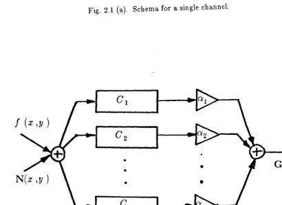
Feedforward pattern classification systems based on multi-channel machines are

introduced. The concept of independent channels is defined and used to generate

independent features. The statistics of multi-channel classifiers are characterised, and

specific applications of these structures are considered. It is demonstrated that image

classification invariant to image rotation and shift is possible using multi-channel

machines incorporating a square-law point rule. The general form of rotation

invariant classifier is obtained. The existence of optimal solutions is demonstrated,

and good sub-optimal systems are introduced, and characterised. Threshold point

rules are utilised to generate a class of low-cost binary filters which yield excellent

classification performance. Performance degradation is characterised as a function of

statistical side-lobe fluctuations, finite system space-bandwidth, and noise.

Simplified neural network models are considered as feedback systems utilising a

linear map and a threshold point rule. The efficacy of these models is determined for

the associative storage and recall of memories. A precise definition of the associative

storage capacity of these structures is provided. The capacity of these networks under

various algorithms is rigourously derived, and optimal algorithms proposed. The

ultimate storage capacity of neural networks is rigourously characterised. Extensions

are considered incorporating higher-order networks yielding considerable increases in

Contents

Acknowledgement

Abstract

Methodology

CHAPTER I

INTRODUCTION

1. Prelude

2. Pattern Classification

A. Canonical Classifiers and Discriminant Functions

B. Linear Discriminant Functions

C. Matched Filters

D. The Capacity of a Separating Plane

E. Generalisations: Linear Maps with Point Rules

3. Associative Memory

4. Measures of Performance

A. Consistency

B. Probability of Error

C. Bhattacharyya Coefficient

D. Normalised Mean Separation

_,.

5. Organisation

-32-Correlators

CHAPTER II

MULTI-CHANNEL MACHINES

1. Finite-Dimensional Feature Spaces

A. System Structure

B. Noise Consideration

C. Statistically Independent Features

2. Quadratic Machines

A. Square-Law Point Rules

B. Single Channel Statistics

C. Multi-Channel Statistics: The Characteristic Function

D. The Cumulants of the Output Probability Distribution

E. An Orthogonal Series Expansion for the PDF

F. The PDF for a Pure Noise Input

3. Threshold Machines

A. Threshold Point Rules

B. Single Channel Statistics

C. Multi-Channel Statistics

References

CHAPTER III

ROTATION INSENSITIVE FILTERS

1. Introduction

A. Background

ti'

B. Quadratic Machines

2. The General Form of Rotation Insensitive Filters

3. Optimal Classification

-76-A. Asymptotic Optimality

B. Existence of Optimal RIPs

4. Sub-Optimal Classification

A. Maximally Separating Rotation Insensitive Filters

B. Comparison of System Performance with Matched Filters References

CHAPTER IV

BINARY FILTERS

1. Introduction

2.

System Models and Performance Measure

A. A Generalisation of the Fourier-Plane Correlator

B. Performance Measure

3.

Signal Statistics

4.

Two-Class Discrimination: No Additive Noise

A. The Matched Filter B. The Binary Filter

C. The Matched Binary Filter

5.

Classification in Additive Noise A. The Matched Filter

B. The Binary Filter

c.

The Matched Binary Filter

6.

Numerical Solutions and Discussion

Appendix A

Appendix B

-159-Neural Networks

CHAPTER V

ASSOCIATIVE NEURAL NETS

1. Neural Network Models

A. Iterated Maps

B. Neurobiological Modeling

2. Associative Memory

A. Association, Attraction, and Tolerance

B. Capacity Definitions References

CHAPTER VI

OUTER PRODUCT NETWORKS

1. The Encoding Algorithm A. The Interconnection Matrix B. Memory Stability

C. Examples

2.

Attraction Dynamics A. Asynchronous Mode B. Synchronous Mode

3.

Capacity Heuristics

A. A Gaussian Conjecture

B. A Poisson Conjecture

4.

Preliminary Lemmas

5.

Capacity: A Tale ¢ Two Lemmas A. Fixed Points

B. One-Step Synchronous Attraction

-231-C. Non-Direct Convergence

D. Error Tolerance

References

CHAPTER VII

SPECTRAL APPROACHES

1. Tailored Spectra for Memory Encoding

A. A New Perspective of the Outer Product Scheme

B. Constructive Spectral Approaches

C. Examples

2. Algorithm Characterisation

A. Features

B. Attraction

C. Modifications and Spectral Choice

3. Computer Simulations

References

CHAPTER VIII

MAXIMAL EPSILON CAPACITY

1. Reduced Model for Error Tolerant Associations A. One-Step Synchronous Associations

B. Error Tolerance C. Definition of Capacity

2. Preliminary Results

A. Technical Lemmas

B. Main Lemmas ,

3.

Epsilon Capacity of Neural Networks A. (Zero )-Capacity

B. Epsilon Capacity

-299-4. Distribution of Errors

A. Strong Convergence to Mean Error Rate

B. Universality of Capacity Bounds

5. Optimal Weight Matrices

References

Extensions

CHAPTER IX

SELECTED PROBLEMS

1. Discussion

2. Binary Interconnections

A. Introduction

B. Majority Rule Based Interconnections

3. Multiple State Neurons

A. Multiple Threshold Point Rules

B. Outer Products Revisited

C. Spectral Approaches

4. Distortion Invariance

A. Generalisation: Outer Product Algorithm

B. Translational Shift Invariance

C. Rotation and Shift Invariance

5. Higher Order Networks

A. Polynomial Maps

B. Outer Products Again

C. Generalised Spectral Schemes

D. Maximal Capacity of Polynomial Maps

-355-Beauty is Truth,

Truth Beauty;

John Keats

CHAPTER I

INTRODUCTION

1. PRELUDE

Linear systems combine the dual advantage of analytical tractability and

implementation simplicity. Consequently, they have found ready application in divers',

problems in signal detection and pattern classification, as well as in allied situations in

associative or content addressable memories. Linear maps together with a non-linear

threshold rule for instance can be fruitfully employed in good classification schemes, as

in Matched Filtration in signal detection. In such schemes the linear map can be viewed as providing communication of information between the various components of

a problem, while the threshold decision rule provides the necessary non-linear

computation adjunct to logical problem solving. The advantages of using linear

transformations in conjunction with a simple decision rule in these situations is clear:

these systems allow of low cost implementations, and their performance can, in almost

all cases, be completely characterised.

The very simplicity of the linear map, however, precludes doing more complex

problems. As an instance, it is not possible to achieve rotation invariance m image

recognition using purely linear maps with a threshold decision rule.

,,.

The approach we will follow is to introduce low complexity generalisations of

linear transformation to include point non-linearities. We demonstrate that the

resultant systems expand considerably the set of problems that can be done using just

pointwise on the domain, all that is needed in addition; is an array of

single-input/single-output non-linear devices if the processing is done in parallel, or a single

such device if the processing is sequential.

We consider applications of this approach to pattern classification usmg two

particular non-linearities: square-law and threshold rules. The problems considered

include: a characterisation of a general class of rotation invariant image recognition

systems, and a performance characterisation of a class of low complexity binary filters.

With the introduction of feedback much more complex behaviour than simple

classification can be realised in such systems. We focus on associative memory as an

application, and obtain precise results on the capacity of simple iterated maps

(comprised of linear transformations composed with a threshold rule) for storing

complex associations.

2. PATTERN CLASSIFICATION

A. Canonical Classifiers and Discriminant Functions

We start with a description of the classical pattern classification problem. Let

{ n(ll, ... , n(c l} be a finite set of c states of nature which we will also refer to as

classes. The states of nature are represented by vectors x in a pattern space IHP. We

will assume throughout that IHP is a subset of an inner product space with the

inherited inner product. We will denote the inner product space containing IHP by

lliP. Instances of pattern spaces that we will use are: the Hilbert space (complex) L 2

of square-integrable functions, the vector space of real n -tuples R" , and the set of

vertices of the binary hypercube {-1,1 }" = ID". (For the first two examples

IHP

=

mp

while for the last example, HIP = IBn while IBP = fil n .) The

occurrence of the patt..ern vectors x E IBP is specified according to the underlying

state-conditional probability distributions

F

x(

I

I

o(s l) = p

{x

EI

I

o(s l} which specify the probability of events { xE IC lllP } conditional upon the occurrence of a

state of nature n(s l, and the a priori probabilities of occurrence, P { o(s l}, of the

various states of nature.

Definition. A pattern classifier is a rule C IllP --+ { f2(1l, ... , n(c l}.

A couple of remarks are in order:

(1)

The classifier partitions the pattern space Illp into c regions corresponding to the

states of nature. Specifically, each feature vector x E IllP is associated with some

state of nature.

(2) Note that we do not lose in generality by specifying the domain of the classifier C

to be all of Illp. We could, for instance, utilise a dummy state of nature f2(o) such

that if x is mapped to n(o) by

c'

then it indicates positive non-recognition of x.

(3) While some simple situations arise when C is constrained to be a fixed mappmg

on the pattern space, we could, in principle, allow C to be a random mappmg

predicated upon some random specification of states of nature. Loosely speaking, in

the first case the states of nature are fixed, and correspond to some fixed partition of

the pattern space. In the second case, partitions of the pattern space corresponding to

the states of nature are themselves chosen randomly. This corresponds to specifying

an underlying probability distribution on the state-conditional probability

distributions F xU I f2(s l) themselves. For this case, a particular realisation of a

classifier mapping C is predicated upon a particular realisation of the state-conditional

probability distributions. We will utilise both forms of classifiers- fixed and

random-fruitfully.

Two issues m re classifiers are their characterisation with regard to some

objective measure of performance (we shall return to this issue in section 3), and the

complexity of their implementation. Before moving on to these two issues, we first

introduce a canonical form for pattern classifiers. Our treatment follows that of Duda

and Hart

[1].

Definition. A set of discriminant functions (for classifier C) is a set of c real valued

functions on the pattern space,

8

8

) : Illp --+ Ill, s

=

1, ... ,c, such that for every

{l.2.1)

if

c

(x)

=

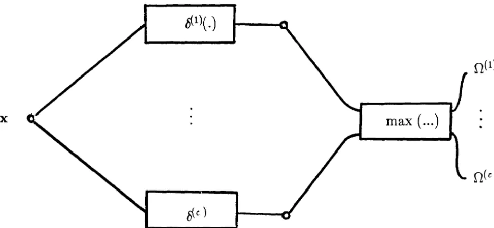
n(I l.

A canonical form for pattern classifiers is a machine that computes c discriminant

functions, and selects the state of nature corresponding to the largest discriminant

function. A block-diagrammatic representation of such a classifier is illustrated in fig.

1.1

The choice of discriminant function 6(8

) for a classifier C is not unique, and m

fact the following assertion holds, as is easily seen.

Proposition 1.2.1. Let

f :

IR --+ lR be any monotonically increasing function.

Then

f

o 6(8

) : llIP --+ JR, s

=

1, ... ,c, is also a set of discriminant functions for

classifier C .

Thus we have an equivalence class of sets of discriminant functions for each

classifier, with each set of discriminant functions yielding the same resultant

classification. While such sets of discriminant functions are indistinguishable from a

theoretical point of view, in practice, however, the appropriate choice of discriminant

functions can lead to considerable savings in analysis and implementation.

In

the discriminant function methodology, the pattern space is partitioned into

c decision regions R (1), . . . , R (c) C lHP , with x E R (t) if

8

1)

>

£/

8) for all s

=/:-

t .

The decision regions are separated by decision surfaces where two or more

discriminant functions take on equal values. Classification of points on the decision

surfaces can be made by using any suitable tie-breaking rule.

,,.

B. Linear Discriminant Functions

In

practice, the cost of realising "optimal" classifiers may well be prohibitive, as

x

fj

c)

Fig. I.I. Canonical classifier: Discriminant function

realisation.

max ( ... )

classifiers of fixed structure. While such classifiers of necessity sacrifice some

performance, they gain in simplicity of construction, and in being relatively easy to

compute.

Linear discriminant functions are classifiers of fixed structure which are affine

linear functionals on the pattern space lHP . These are particularly attractive

classifiers from the computational point of view as they are among the simplest

non-trivial classifiers to implement, and are very tractable analytically. They are even

optimal classifiers for an admittedly small set of underlying distributions. As such,

linear discriminant functions are attractive candidates for classifiers.

We will denote the set of c linear discriminant functions corresponding to a

linear classifier (also called a linear machine) by the functionals L(8) : lHP -+ IR,

s

=

I, ... ,c. With each L(8) we associate a weight vector 1(8) in the parent inner

product space IlIP , and a real scalar threshold I

d

8

) , so that for every pattern

x E IlIP,

(I.2.2)

Pattern classification is by means of the threshold comparison rule of equation (1.2.1).

Note that for the two-class case, this is just a threshold rule: decide 0(1J zf ( 1(1) - 1(2) , x )

+ (

l ₀(l) - I ₀(2) )

>

0, else decide 0(2l.

Denoting the c -tuple of linear discriminant functions by

L

=

(01_{), . . . , L(c)): lHP}

-+ IR.c, and the comparator of (l.2.1) by

T : IR c -+ { 0(1l, ... , o(c l}, the linear classifier C can be written as the composition

(To L ) : lHP -+ { 0(1), ... , o(c l}. A two-dimensional illustration of possible

decision regions produced by such a linear machine is shown in fig. 1.2.

Extending the analogy of fig. 1.2 to higher dimensions, each linear discriminant

can be thought of as ~alising a separating plane (hyperplane) in a multi-dimensional

space. The decision surfaces of the linear classifier are c separating planes, and these

F;g_ 1.2. Parth;onfog of pattern space by a linear

C. Matched Filters

A particular instance of a useful linear classifier is the matched filter. We

illustrate this with an example in signal detection. We are presented with a situation

where a signal or reference pattern x₀ E IllP , may or may not have been present in an

environment of additive, zero-mean noise, with a positive definite autocorrelation

operator Rn : IllP -+ lip . There are two states of nature corresponding to the two

hypotheses: the presence or absence of the signal. Given a pattern x E IllP, (whose

state-conditional probability distribution is determined by the random n01sy

environment, together with the presence, or absence, of the signal) the problem is to

find suitable weight vectors to achieve a reliable mapping of x into one of the two

states of nature.

The matched filter is a weight vector (corresponding to a linear discriminant

function) defined by

I

A 1D -1

- Jn.n Xo · (1.2.3)

If the noise is white, as is frequently assumed, then

i

is just a scaled version of the

signal-hence the sobriquet "matched" filter. Note that as there are only two states of

nature, it suffices to have a single linear discriminant function corresponding to the

hypothesis that the signal was present, with a simple threshold classification rule.

The fact that makes the matched filter important is the following classical

result. Let HIP denote the space of positive-definite noise-autocorrelation operators.

Define the signal-to-noise ratio (SNR) functional p: Ilf P X HIP X JfIP -+ Ill+ by

1(1,x)\2

p ( x ,1 ,Rn ) =

~~~-( I , Rnl )

,

(l.2.4)

Theorem 1.2.1. For a fixed signal Xo E mp' and a fixed positive definite

no1se-auto-correlation operator, Rn E JfIP , the matched filter

i

E llIP maximises the

We shall return to the issue of signal-to-noise ratios again in Section 3 when we

consider performance measures for classifiers. The signal-to-noise ratio is a frequently

employed performance measure because of its simplicity, and in some cases it is

actually a good measure of classification performance. With the signal-to-noise ratio as

a criterion then, the matched filter provides the best performance among all linear

discriminant functions. The idea can be simply extended to multiple discriminant

functions in the c -class recognition problem.

D. The Capacity of a Separating Plane

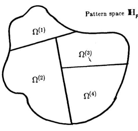
In spite of their many appealing features, however, linear discriminant functions are intrinsically limited in scope. The decision regions for a linear machine are

constrained to be convex, and this in particular leads to the fact that every decision

region must be simply connected. These factors seem to imply that the linear

discriminant function approach is best suited for situations where the state-conditional

probability densities are unimodal, i.e., the presence of a particular state of nature

results in patterns which are clustered together locally in the pattern space, as

illustrated in fig. 1.2. An instance where this fails is in image recognition. Associate

all rotations and scales of a reference image with one class or state of nature. The

patterns in the class are not clustered together in the image space, so that linear

discriminant functions do not work well in this instance.

A more serious limitation of linear discriminant functions is that they are

seriously limited in the num her of states of nature that they can accurately classify.

Consider a finite-dimensional Euclidean pattern space, which we take to be ffi11

without loss of generality. Let x(ll, ... , x(c l be c reference patterns in

nr

chosen to be in general position (i.e., any subset of n or fewer reference patterns is linearly

independent). At the very least, we require that the reference patterns themselves be

mapped to the appropriate states of nature.

,

The weight vectors I corresponding to linear discriminant functions are just n

-tuples of real numbers, and the inner product- is the natural one. For this case we

n

L(x)=(l,x)+lo=

:E

l;x; +lo.

j = l

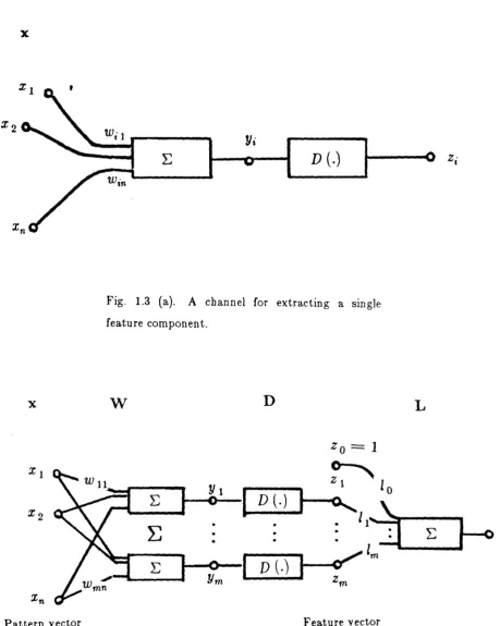
For the two-class case, for instance, this leads to a simple threshold decision rule, as

illustrated in fig. 1.3 (a).

We query: how large can the number of classes c be made while ensuring that

3

some set of linear discriminant functions which accurately maps the reference

patterns to the appropriate class? The answer is furbished in the following result

which we prove in chapter IX (also cf. [2]).

Theorem 1.2.2. For every A E (0,1), as n - oo, the probability that

3

a linear

discriminant function which accurately classifies the c reference patterns approaches

one if c

<

2(n

+

1)(1 - >..),and approaches zero if c

>

2(n

+

1)(1

+

>-).

Thus, no more than 2 ( n

+

1 ) states of nature can be accurately identified by linear discriminant functions if the pattern space is an n -dimensional Euclidean vector

space. This result is consistent with an argument based on the available degrees of

freedom: the n -dimensional weight vector together with the scalar threshold cons ti tu te

n

+

1 degrees of freedom. If we need more powerful classification capability, and

more flexibility in classification, however, we will have to resort to more complex

classifiers.

E. Generalisation: Linear Maps with Point Rules

We consider generalisations of the linear discriminant function structure which

allow of more flexible classifiers, but which at the same time retain much of the

simplicity of linear machines. Our approach is to introduce a "feature extraction"

stage prior to actually computing linear discriminant functions, as is indicated

schematically in fig. 1~3. The feature extraction procedure is a composite mapping

from the pattern space _{llIP to a feature space lH / . The linear discriminant functions}

x

X2

x

wil

Yi

D (.)

Win

Fig. 1.3 (a). A channel for extracting a single

feature component.

w

D

Pattern vector

Fig. 1.3 (b ). Realisation of a generalised linear discriminant

function.

Z· _l

The feature spaces we consider are vector spaces indexed by some set. Specifically, lH _/ is a family of real-valued functions y : A-+ JR satisfying some suitable properties (such as continuity or square-integrability), where A is some index set. The following are two examples of feature spaces.

Example 1. Choose _{lH /} to be the space of all square integrable real-valued functions

on the twcr-dimensional plane. The underlying index set in this instance is A

=

R2.

D

Example 2. The vector space of real m -tuples Rm , which is indexed by the finite set

A= {l, ... ,m }. D

We will use the representation

(y

_{11 :} 11 EA) to explicitly represent feature vectors

y _{E lH /} in terms of the underlying index set A. We denote the (parent) space of

complex-valued functions indexed by A by lH _{1 ,} and assume that lH ₁ comes equipped with an inner product.

Definition. A map D : IH / --+ _{IH / is a} point rule (on the feature space) iff there is

a function D : ~-+ R such that

(l.2.5)

If the indices 11 represent time, for instance, then the point rule D 1s a memoryless

map.

Example 8. (Square-law point rule)

D(y II: v EA)

= (

I

y 11) 2 : II EA). D

Example

4.

(Threshold point rule)

Point rules are interesting from a practical point of view, as they are reasonably

simple to implement-each vector component generated by a point rule depends solely

on the corresponding component of the original vector. Point rules may be realised in

parallel by a family of identical single-input, single-output devices (or sequentially by a

single such device).

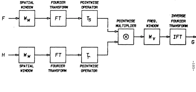
The feature extraction procedure that we will consider throughout is a

composite map (Do W): IHP - _{IH1 ,} where W: IHP - _IH1 is a linear map, and

D : IH_{1 -} IH₁ is a point rule.

(In

some cases, we could think of the feature-extraction procedure as being a dimensionality reduction process which effects a

sensible reduction of a pattern space of high dimensionality to a lower dimensional

feature space.) The final classification stage is by means of discriminant function on

the feature space _{L: IH1 - Dl.}

We will refer to the feature extraction procedure for each component z v of the

feature vector as a channel. If the feature space is m dimensional, we will have m -channels to compute the components of the feature vector.

Thus, the discriminant functions that we will be considering are of the form

(Lo Do W) : IHP - Dl. These discriminant functions 'may be considered to be simple generalisations of linear discriminant functions involving the point rule D.

Note that the particular choice of D =Id results in a simple linear discriminant

function (Lo W) on the pattern space. Thus these new constructs are generalisations of linear machines, which encompass linear classifiers. Additional

flexibility in classification is obtained by suitably specifying the (generalised) decisions

D, and the linear maps W, and L. If D is a threshold map, for instance, the

procedure is akin to making several partial decisions at an intermediate stage, and

using these as features to obtain a final classification using a linear discriminant

function.

,

In fig. 1.3 (b) we have a schematic representation of these generalised linear discriminant functions. The pattern space for this example is Euclidean n -space,

while the feature space is Euclidean m -space. Pattern vectors x E

m.n

are mapped to

n

vectors

y

E lRm

by

an m

X

n

matrix of

weights [

wii ],

with

Yi =

E

u';i xi. The

point rule D acts pointwise on each component Yi to produce an m -vector z with

components zi =D (Yi)· Finally, the discriminant function is formed as a linear

m

combination

E

li zi

+

1₀ of the components of the feature vector z.

i =l

As pointed out earlier, these generalised constructs subsume within them the

linear discriminant functions as a trivial case. A proper choice of point rules allows of

some added flexibility in classification. We illustrate this in the following example.

Example 5. Consider the Boolean mapping XOR: { 0,1} X { 0,1} - { 0,1},

(x i,x

2)

= (1,0)

(x vx

2)

=

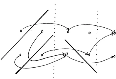
(1,1) ·

The logical XOR is a two-state classification problem which cannot be realised by any

linear discriminant function. As illustrated in fig. 1.4 (a), there is no choice of

separating plane which isolates points (0,0) and (1,1) from points (0,1) and (1,0).

However, a generalised linear discriminant function using a threshold point rule can be

constructed to solve the problem, as illustrated in fig. 1.4 (b ). Here, Boolean pairs (x ₁₇x ₂₎ are first mapped into a two-dimensional Boolean feature space through the

linear map with component matrix

[ 1 -2]

w

=

-2 1 '

and a point rule based on the threshold map

D ( ) _{y = {}

o

_I if _if y _y

_>

<

o.5

_{0.5 .}

,.

(0,I)

0

(0,0)

0

Fig. 1.4 (a). No choice of separating plane can separate (0,0) and

(1,1) from (0,1) and (1,0).

It can be easily seen that this procedure maps (0,0), and (1,1) to (0,0), while mapping

(0,1) to (0,1), and (1,0) to (1,0). Finally, constructing a linear discriminant function

with weight vector I=

0),

and threshold I ₀

=

-0.5, on the feature space results in the map

This is the required logical XOR.

o

Another instance of this acquired flexibility is examined in chapter III, where we

analyse the problem of image classification invariant to image shift and rotation in

some detail. This is a problem which can be solved via generalised linear discriminant

functions, but which linear discriminant functions cannot solve in isolation.

Simple point rules are favoured from the implementation point of view. In the next few chapters, we will examine classifiers of the above structure using simple point

rules under a variety of conditions. Note, however, that with classifiers of this

structure, the linear discriminant function at the feature space determines the actual

number of states of nature that can be identified. Thus, if the feature space is an m

-dimensional Euclidean space, we can classify at most 2( m

+

1) patterns by theorem (1.2.2). Thus, with a feedforward system of the sort we have been considering so far,

we can achieve more flexibility in classification, but cannot really improve significantly

on the capacity of the classifier (over a linear machine) unless we allow of feature

spaces of large dimensionality. This of course is in accordance with intuition-to solve

,

complex problems we will need a great number of degrees of freedom, which in this

case corresponds to large feature spaces. The best gains, as we shall see, will accrue

from dispensing with the linear discriminant function stage, and considering cascades

3. ASSOCIATIVE MEMORY

A problem allied to that of pattern classificati9n is that of associative or

content-addressable memory. Formally, an associative memory is a classifier where

the states of nature are themselves specified patterns from the pattern space.

Specifically, an associative memory is a map from the pattern space to itself, which

maps a subset of the pattern space to a specified set of pattern vectors

{ u(1l, . . . , u(m l } . The specified set of vectors are called the fundamental memories.

In a typical problem in associative memory, we specify a "similarity" metric for

the pattern space, and require that the associative memory maps all patterns which

are near a fundamental memory to the memory itself.

Example 6. Consider a pattern space of binary n -tuples, IBn. Let the specified metric

be the Hamming distance between two vectors, and let 0

<

pn

<

~ be the specified

extent of similarity. For a set of m fundamental memories, u(a) E IBn, a= l, ... ,m,

which are mutually separated by Hamming distances greater than pn, we require that

all vectors in Hamming balls of radii pn surrounding the fundamental memories be

mapped to the corresponding memories. 0

We hence require an associative memory to be a nearest-neighbour pattern classifier, or

equivalently, an error correcting code. Note that it may not be absolutely essential

that the associative memory map patterns to precisely the fundamental memories. If a

certain measure of error tolerance is prescribed, for instance, it may suffice that the

mapping results in any of a number of patterns near the fundamental memory.

System-theoretic approaches to associative memory have benefited greatly from

neurobiological modeling of brain function, and much of the terminology, and

approaches in vogue have a strong biological flavour (cf. [3]). Hence, while an

associative memory is formally a pattern classifier, we will nevertheless distinguish

Correlators), and problems in associative memory (which we treat in the section on

Neural Networks). For the pattern classification problems we will consider generalised

linear machines of the form we introduced earlier. For associative memory, however,

we require maps from the pattern space to itself. We hence dispense with the linear

discriminant function classification stage, and consider iterated maps of the form

(Do W)k : IHP -+ JHP, where W: JHP -+ IHP is a linear map, and D : JHP -+ JHP

is a point rule.

Thus, the pattern classifiers we consider are feedforward systems which make

hard decisions upon vectors in the pattern space through the medium of the

generalised linear discriminant functions. Clearly, if an error is made in the decision process, then the classification is irretrievably in error. The associative memory

structure we consider is a feedback system, and hence has the potential to compensate

for occasional errors in decision. In this case, the iterated mapping considered on the pattern space makes soft decisions which gradually converge to a true classification

decision. We will elucidate upon this in greater detail in the section on Neural

Networks.

4. MEASURES OF PERFORMANCE

A. Consistency

Thus far, we have alluded only briefly to criteria for judging performance.

Objective measures of classifier performance are, however, of prim a facie importance in

characterising classifiers and rating their relative performance. We will, in main, not

distinguish between classifiers and associative memories in this section. The

performance measures we develop for classifiers will continue to hold for associative

memories as a special family of classifiers.

I'

Let 6. denote the family of discriminant functions. By equation (l.2.1), a c

-tuple of discriminant functions ( 6(1), . . . , 8(c l) E 6. c represents a particular

Definition. A performance measure for classifiers is a mapping p : ..:'.). c - IR which

induces a linear order (>) on the sets of discriminant functions corresponding to

classifiers. We shall say that a classifier realisation ( tf...Il, . . . , ftc)) is superior to a

classifier realisation (~,Pl, . . . ,

1c))

with respect to a performance measure p if

p( [fl)

1 • • • 1 o(c))

>

p ( 11)1 • • • 1 1(c) ).

Clearly, an arbitrary definition of performance measure is unlikely to subscribe

to our intuitive notions of what a good classification scheme entails. If the

performance measure is to reflect some "true" measure of goodness of various

classifiers, then it must be chosen with some care, and in particular, must reflect the

underlying a priori probabilities of the states of nature and the state-conditional

distributions of the pattern vectors. Before returning to the issue of what constitutes

a good performance measure, we first characterise some desirable consistency

properties in performance measures which will be useful in classifying different

measures.

As we saw earlier, there exist an infinity of sets of discriminant functions

satisfying equation {l.2.1), all of which represent a particular classifier. Hence, with

every specified classifier

c :

llip - {

o(ll, ... ' ore) } '

we have an associated equivalence class of c -tuples of discriminant functions, Sc = [ (tPl, ... ,tJc) )c ], with

each member of Sc realising the same mapping {specified by the classifier C) from the

pattern space to the set of the given states of nature. A desirable consistency property

of the performance measure is that it be insensitive to the specific discriminant

function realisation of a classifier, so that the classifier order relations are invariant to

implementational details.

While total consistency is clearly a very desirable property in a performance

measure, we might suspect that this would place too rigourous a constraint on

permissible performance measures.

In

fact, as can be seen from the following assertion, totally consistent performance measures have to be explicitly representable as

functions of partitions of the underlying pattern space.

Let P be the family of all partitions of the pattern space Il1P into c disjoint

subsets. For every classifier C, let Re

= {

R (i), . . . , R (c)} be the induced

partition of Il1P; specifically, x E R (a) ~ C (x)

=

O(' ). Let g : Ac --+ P be the

natural mapping associating c -tuples of discriminant functions with partitions of the

pattern space; g ( b(l), . . . ,

tJc))

=

Re whenever (

tJ

1_{), . • • ,}

_tJc))

_{is a member of}

the equivalence class Sc of discriminant function c -tuples corresponding to classifier

c.

Proposition 1.4.1. A performance measure p : Ac --+ R is totally consistent iff 3 a

mapping µ : P --+ IR such that p

=

µ o g .

Proof. Assume

3

a map µ : P --+ IR such that p

=

µ o g . Let C be a classifier.

Every discriminant function c -tuple in the equivalence class Sc is mapped into the

same partition Re of HP by g . Hence, p

=

µ o g is totally consistent.

Now fix a classifier C, and assume p is a totally consistent performance

measure. Let ( lPl, ... ,

tJc})

be any member of Sc. Now, every partition in P

corresponds to some classifier. Define the map µ : P --+ IR by

µ (Re )

=

p (( b(ll, ... ,

tJc}

)c ) for every partition Re in P. Then p = µ o g.

o

The restriction that p be specified in terms of partitions of the pattern space

can be quite unrealistic, especially for large (infinite!) dimensional pattern spaces.

From a practical stanflpoint, we would like to be able to specify the performance

measure directly m terms of the "observables," the discriminant functions.

Definition. A performance measure p is monotonically consistent iff for every

monotonically increasing, piecewise differentiable function

f :

R - R, and every c

-tuple of discriminant functions (

8

1), .. .,{}c)) E ~ c,

p ( 81_{), . . . , 9c))}

₌

_p(

_J

₀

_{tf..ll, ... ,}

_J

_{0 9c) ) .}

We introduce the requirement of piecewise differentiability in the definition to allow of

some ease in proving technical results later. The requirement restricts our attention to

"useful" functions

J .

Monotonic consistency is clearly not as strong as total consistency, and in fact,

totally consistent performance measures are also monotonically consistent. The

converse is not true, however. Nevertheless, in light of proposition (1.2.1),

monotonically consistent performance measures exhibit consistent behaviour over a

useful range of discriminant function realisations of classifiers.

We now return to the issue of specifying good performance measures which we

hope are consistent in some sense. In the remainder of this section we will specify three measures of performance to which we will frequently have recourse.

B. Probab£l£ty of Error

In line with intuitive expectation, a good performance measure will reflect the

underlying a priori probabilities of the states of nature, and the state-conditional

probability distributions of the pattern vectors. We illustrate with an example.

Assume the state-conditional distributions are such that the occurrence of any

pattern vector depends solely on the presence or absence of one of the states of nature.

In effect, the state-conditional distributions are localised in disjoint regions in the

pattern space. This is shown schematically in fig. 1.5 (a), where we assume four states

of nature. Here, P ( ~

I

fl(')) is identically zero outside the indicated support for the probability distribution conditioned on O(' l. Now assume we have a classifier C

which partitions the pattern space into c regions, as illustrated in fig. 1.5 (b ). The

partitions here are indicated by bold lines. Clearly, ideal classifier performance would

Pattern space

H,,

Fig. 1.5 (a). A partition of the pattern space according to prescribed state-conditional probability distributions; a pattern in a particular region will occur only if the corresponding state of nature occurs.

Pattern space

H

₁₁

..._.., ___ ... c., ..

>

f1(3)

..

·

Fig. 1.5 (b ). A partition of the pattern space by a particular classifier. The shaded areas denote regions with non-optimal

the boundaries demarcating the support of the state-conditional distributions in fig. 1.5 (a). For the indicated classifier, however, there is a mismatch in the decision boundaries, as indicated in the hatched areas in the figure. Vectors in the hatched areas are erroneously identified by the classifier: in particular, some vectors arising from f2(2) are mistakenly identified with f2{1l, while some vectors arising from

n{

3) are associated with f2(4l. A true measure of the performance of the classifier is hence the extent (area) of the hatched area of erroneous classification, suitably weighted by appropriate a pri'ori probabilities. Performance, in general, would be deemed to improve if the hatched area decreases in size. More generally, optimum classifier performance is obtained if classification is according to the largest a posteri'ori probability, P { f2(8

)

I

x}.

This results in the Bayes classifier, which unfortunately,

takes on a simple form only in exceptional cases. In general, for discriminant functions of the fixed parametric form that we consider, the resultant classification performance

will be suboptimal. The probability of error for such classifiers tells us the extent to which we have sacrificed optimality by electing to look at relatively simple parametric structures for discriminant functions.

We generalise this approach to allow of arbitrary state-conditional distributions and a priori probabilities for the states of nature.

Let C be a classifier, and let Re

= { R

(I), . . . , R (c) } be the partition of

ffiP induced by C. Let the state-conditional probability distributions be denoted by F (I

I

n8 )

=

p { x E I

I

f2(8

) } for measurable sets I

c rnp '

and let

11'(8 l

=

P { n(s l } denote the a priori probabilities of occurrence of the various states of nature. Then the probability of {classification} error, Pe, is defined as

c

Pe !:,. 1 -

E

rr( 8 l

J

dF ( x 1

n (

8 J ) .

B=l n(•) (1.4.1)

""

Each term in the sum is just the probability that a particular state of nature occurs,

error occurs in classification is clearly one minus this probability.

The probability of error (or more precisely, the probability of correct classification) is the ultimate performance measure for classifiers. It tells us the

expected losses that accrue from the usage of any particular classifier. (In decision-theoretic terminology, the probability of error is the expected risk corresponding to a 0 - 1 loss function.)

Proposition 1.4.2. 1 - Pe is a totally consistent performance measure.

Proof. The proof follows directly from equation (1.4.1 ), and proposition {1.4.1 ). D

The probability of error hence imposes an absolute linear order on classifiers, and the goodness of other performance measures depends on how closely they approximate Pe. In practice, however, Pe is frequently too difficult to calculate unless

the underlying distributions are cooperative. We hence introduce two more measures of performance.

C. Bhattacharyya Coefficient

We will restrict ourselves to the two-class case for simplicity in the ensuing exposition. Let o(I) and 0(2) be the two states of nature with a priori probabilities 7r(I) and 7r(2l, respectively. Let 8 be a discriminant function with the classification rule:

x r-+ o(ll

x t-+ 0(2)

if 8 ( x )

>

0

if 8 ( x)

<

0 .

(Note that for the two-class case, it suffices to consider a single discriminant function. Specifically, if fJ{I) and

8

2) discriminant functions as in (l.2.1), then set 8 = fJ{I) -

8

2l.)

!'

The discriminant function 8 is a random variable whose distribution is conditioned upon the states of nature o(ll and 0(2_{l. Assume the class-conditional}

00

PB A ( 11"(1)J2J)1/2

J

{P ( v

I

n(l)) P ( v

I

n(2)) p12 dv . _(1.4.2)

-00

In actuality, the Bhattacharyya coefficient ranks classifiers in inverse order. An appropriate performance measure ranking classifiers in their proper order is the

Bhattacharyya distance dB = - In PB. As there is a 1-1 correspondence between dB

and PB, however, we will continue to use PB as a performance measure with the

understanding that classifier ranking is reversed.

The Bhattacharyya coefficient is much simpler to compute than the probability

of error as it does not require the explicit specification of the various decision regions.

Furthermore, it is a good performance measure in the sense that it bounds the

probability of error fairly tightly.

Proposition 1.4.3.

! (

1 -

JI - 4pff)

<

Pe

<

PB .

Proof. The proof is as in Ref. [5] with a slightly different definition of PB.

Proposition 1.4.4. PB is a monotonically consistent performance measure.

Proof. Let 8 be a discriminant function with Bhattacharyya coefficient PB given by

equation (1.4.2). Let

f :

Ill - IR be a monotonically increasing function. For

simplicity assume

I

-l is differentiable. Let p " ( v

I

n(s))

denote the probability density function of

J

o 8 conditioned upon the presence of

nrs

l for s

=

1,2, and let

p;

denote the associated Bhattacharyya coefficient. We have

,.

The support of

J

o 8 is contained in the open interval(! (-oo),f (oo)). Hence,

/(811)

p

B

= (

7r(l)rr(2

l)1

12

I

{p " (

v

I

n(l))

p " (

v

I

nr

2

l)}

l/Z

dv

= (

,fl)11"(2))1/2

J

I (oo)

{p

(!

-1( v)

I

o(ll) p

(!

-1( v)

I

0(2)) }1/2 df

~~

v) dv

I

(-oo)

00

= (

11"(1)11"(2))1/2

J

{p (

v

I

0(1)) p ( v

I

0(2)) }1/2 dv -00

=PB· 0

The usage of Bhattacharyya coefficient as a performance measure, hence results m a consistent ranking of classifiers which is not too far removed from the optimal classifier ordering by means of the probability of error as performance criterion. In

fact, it can be shown that Pe approaches PB in the limit of low probabilities of error

[5],

so that in the region of low errors which we are primarily interested in, PB is

actually a very good performance measure.

D. Normalised Mean Separation

We will sometimes encounter situations where both the probability of error, and the Bhattacharyya coefficient are too cumbersome to compute. We hence introduce a variation of the signal-to-noise ratio defined in equation (1.2.4). Again, we consider the two-class case for simplicity, and assume the states of nature are equi-probable.

Let

f/

8

l, s

=

1,2, be the discriminant functions for the two-class case. Define

and

T/(e) =Var (8(8

)) , s = 1,2. (1.4.3)

(1.4.4)

The normalised mean separation is related to the signal-to-noise ratio defined in

equation (1.2.4). Specifically, the normalised mean separation p is one-half the

signal-to-noise ratio when the two states of nature are the presence and the absence of a

deterministic signal in an additive noise environment.

The performance coefficient, p, is not consistent in either of the two senses we

have defined. Hence, its efficacy is likely to be limited to ordering classifier

performance as parameters are changed within fixed functional forms of the

discriminant function. However, it has the virtue of simplicity, and can be easily

computed in most cases. Besides, under limited circumstances, p provides a reasonably

accurate measure of performance.

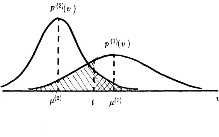
Let 8 denote the discriminant function, with pattern vector x being assigned to

f2(l) if 8(x)

>

0, and to f2(2) if 8(x)

<

0. It is intuitively clear that with such a decision rule classification performance improves if the mean difference between the

correlation peaks of the two classes, µ(l) - µ(2) is made large, and the peak side-lobe

variances, T/(I) and T/(2) are small; specifically, for such a case we can find a suitable

(optimum) threshold t (nominally between µ(I) and µ(2l) which is several standard

deviations from both µ(I) and µl2l. The Bayesian risk-or more specifically, the probability of erroneous classification-hence tends to decrease when the average

inter-correlation peak, µ(ll - µl2l, increases and the side-lobe variances, 77l1l and 77(:!), decrease.

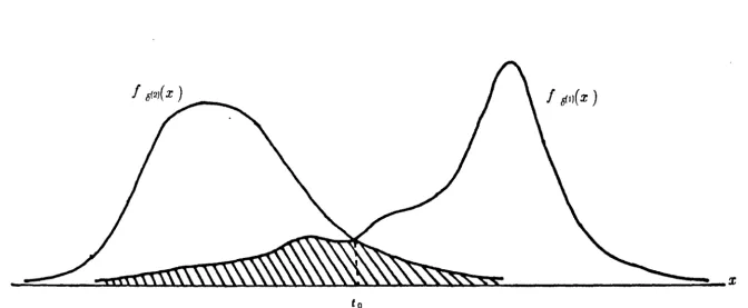
As an instance, the choice of an optimum threshold t for the case of two unimodal

probability density functions

J

#1) and

f

92) is illustrated in the schema of fig. 1.6: the

probability of error (assuming equal a priori class probabilities) is proportional to the

area of the shaded region in the figure.

~

The coefficient p defined by equation (1.4.4) increases monotonically with

increase in the average peak separation, and decrease in side-lobe variance; in this

regard then, the behaviour of p is similar to that of the probability of error, Pe, so

I

bflJ(

x )

~-ssss\\\\~\\\\\\\\\\\\~~sr

~

x

to

Fig. 1.6. A choice of optimum threshold, t 0 , given the two class-conditional densities

f

tf,l)(x ), and

f

{f.zi(x ). The shaded area is the minimum attainable probability of

misclassification.

I

N \0

performance coefficient p is an ad hoc measure that we adopt because of its simplicity and the sustaining arguments above. In the general case-and especially in the instance of multi-modal densities-it is not necessary that the probability of error, Pe , be

expressible as a monotone function of p. A simple case where Pe is indeed a monotone function of p is when the system outputs conditioned on the two classes, G;

,i

=

1,2,

are Gaussian with equal variances v. Then, assuming equal a priori class probabilities,

P,

=~ (-~)'

where <l>(x) is the cumulative Gaussian distribution function

1/2

1 :r

-4>(x)

=

~

J

e 2 dy

v27r _--00

As we shall see later (cf. [5] also) the Bhattacharyya coefficient is also representable as a monotone (decreasing) function of p when the class-conditional distributions of 8 are Gaussian, and the a priori probabilities of the two classes are the same.

5. Organisation

The dissertation is organised into four sections: Problem Methodology, tackled m the introductory chapter; a section on Correlators (chapters II, III, and IV) dealing with particular applications of the proposed generalised linear discriminant functions to specific problems in image and pattern recognition; a section on Neural Networks (chapters V, VI, VII, and VIII) considering problems in associative memory under a suitable iterated map; and finally, a concluding section (chapters IX and X) detailing some extensions and op~n problems.

In chapter II we characterise the statistics of multi-channel classifiers realising

random noISe environment. We introduce the concept of independent channels, and

obtain necessary and sufficient conditions for realising independent channels. We also

characterise discriminant function statistics in some detail when the point rules are

chosen to be square-law of threshold.

In chapter III we consider the problem of achieving image recognition invariant to rotations and shifts of images. We demonstrate that square-law point rules in

conjunction with suitably chosen linear transformations yield discriminant functions

which are invariant to image rotation, and obtain the general form for such systems.

Applying the derived statistics from chapter II, we demonstrate the existence of

optimal rotation invariant image recognition systems with respect to the performance

measure PB. We also demonstrate good sub-optimal rotation invariant classifiers, and

characterise the performance sacrificed to gain rotation invariance.

In chapter IV we consider the usage of point threshold rules in conjunction with linear maps to realise certain classes of binary filters which yield considerable savings

in system complexity and cost. We demonstrate that these classes of binary filters also

yield very satisfactory performance.

Chapter V introduces the form of associative memory structure that we

consider, and elucidates neurobiological terminology, and notation. We make precise

the notion of capacity of these structures, and identify desired properties and

parameters.

In chapter VI we analyse in depth a particular algorithm for memory storage

based on the outer products of the desired memories. We demonstrate that the

dynamics of the algorithm are such as to emulate a physical content addressable

memory, and provide heuristics to estimate its capacity. We then provide

fundamental results with rigourous proofs estimating the storage capacity of the

algorithm under a variety of preconditions.

In chapter VII '#e describe alternate algorithms for memory encoding based on

spectral approaches which intrinsically store close to the ultimate capacity of the

associative network structure itself. We describe various features of the spectral

In chapter VIII we present the derivation of the maximal storage capacity of the

associative network structure when all algorithms are allowed for consideration. The

results bound the performance of any specified algorithm, and take into consideration

specified tolerances of error.

Extensions of the basic neural networks structure as embodied in chapter VI

through VIII, are considered in chapter IX, and particularly in regard to

generalisations of the network to incorporate more communication, and computation,

and the gains in capacity thereby, associative memory architectures using distributed

non-linearities to compensate for specified distortions, and networks using binarised

links. Chapter X concludes with some open problems and questions, and indicates

possible lines of research.

References

[l]

R.O. Duda and P.E. Hart, Pattern Classification and Scene Analysis. New York:

Wiley, 1973.

[2] R.O. Winder, "Bounds on threshold gate realizability," IEEE Trans. Elec. Comp.,

vol. EC-12, pp. 561-564, 1963.

[3] G. E. Hinton and J. A. Anderson (eds.), Parallel Models of Associative Memory.

Hillsdale, New Jersey: Lawrence-Erlbaum, 1981.

[4] A. Bhattacharyya, "On a measure of divergence between two statistical

populations defined by their probability distributions," Bull. Calcutta Math. Soc., vol.

35, pp. 99-109, 1943.

,

[5] T. Kailath, "The divergence and Bhattacharyya distance measures m signal

Correlators