Closed-loop identification using quantized data

(1)

USING QUANTIZED DATA

A thesis subm itted to the U niversity o f L ondon

for the degree o f

Doctor of Philosophy

by

M eihong W ang

U niversity C ollege London

D epartm ent o f Electronic and Electrical E ngineering

T orrington Place London W C IE 7JE

(2)

INFORMATION TO ALL USERS

The quality of this reproduction is dependent upon the quality of the copy submitted.

In the unlikely event that the author did not send a complete manuscript and there are missing pages, these will be noted. Also, if material had to be removed,

a note will indicate the deletion.

uest.

ProQuest U644174

Published by ProQuest LLC(2016). Copyright of the Dissertation is held by the Author.

This work is protected against unauthorized copying under Title 17, United States Code. Microform Edition © ProQuest LLC.

ProQuest LLC

789 East Eisenhower Parkway P.O. Box 1346

(3)

(4)

It is thanks to Nina Thornhill that these three years as a PhD student in Uni versity College London and Imperial College London have been most en joyable. Thank you for consistent encouragement, support and help, and for

being a wonderful thesis supervisor.

I would like to acknowledge The Centre for Process Systems Engineering in Imperial College of Science, Technology and Medicine for sponsoring this research and funding me for three years. The Centre is really a nice aca demic environment for PhD research with so many research active staff and students such as Vassilis Kosmidis, Vassilis Sakizlis and Marcus Vinicius and Thomas Apelt. Thank you for the helpful discussions and the social talks.

Thanks also go to Sirish Shah, Biao Huang and Bhushan Gopaluni of the Computer Process Control group in The University o f Alberta in Canada for the permission to use and help on using the pilot plant for the experimental work during the days when I was there.

(5)

A model of a system is important for applications such as simulation, prediction and control. Closed-loop identification (CLID) is a means of identifying a process model while the process is still under feedback control. The motivation of this project is to find a way to do closed-loop identification while causing minimum disruption to the controlled process.

There are two main categories of closed loop identification. One is closed-loop identification with external excitation (Ljung 1987, System Identification: theory fo r the user, Englewood Cliffs, NJ: Prentice-Hall). Another is relay identification (Âstrôm and Hagglund 1984a, Auto matic Tuning of Simple Regulators with Specifications on Phase and Amplitude Margins,

Automatica, Vol.20, No.5, pp645-651). The first achievement of this thesis is the establishment of a connection between previously unrelated facts by comparing the two main categories of closed loop identification methods. Their advantages and disadvantages were highlighted through case studies.

The second, and the main achievement of this thesis is to propose a new closed-loop identifica tion scheme for a single-input-single-output (SISO) control loop. It is based on a quantizer in serted into the feedback path. The novel contribution of this thesis is to bring the closed-loop identification with external excitation method and the relay identification method into a unified framework for the first time. It gives recommendations about the appropriate method to use for a given quantizer interval. When the quantization interval is small, the quantization error is per sistently exciting, equivalent to an external excitation. The two-stage (step) method can be ap plied. When the quantization interval is large, the relay method can be applied instead. Nonlin earity caused by the quantizer is analyzed, which indicates that nonlinearity increases with the quantization interval. Simulations and experiments showed that the proposed closed-loop iden tification scheme based on quantization is successful.

(6)

A ck n o w led g em en ts 3

A b stra ct 4

Table o f C on tents 5

L ist o f F igu res 12

L ist o f Tables 15

N om en clatu re 16

1 IN T R O D U C T IO N

1.1 O verview 18

1.1.1 An example 18

1.1.2 Motivation 18

1.2 D efinitions and concepts 19

1.2.1 Basic definitions 19

1.2.2 System identification definitions 19

1.2.3 Closed-loop identification (CLID) 24

1.2.4 Closed-loop identification with external excitation 26

1.2.5 Relay-based identification 27

1.3 Problem analysis and key issues 28

1.3.1 Problem analysis 28

1.3.2 Key issues 29

1.4 O utline o f the approaches 30

1.4.1 Case study 30

1.4.2 Simulation 31

1.4.3 Experimentation 31

(7)

2.1 C losed-loop identification with external excitation 33

2.1.1 Introduction 33

2.1.2 Motivation 34

2.1.3 Framework of approaches and methods 34

2.1.4 Specific approaches and methods 37

2.1.5 Closed-loop identifiability, accuracy and efficiency 39

2.1.6 Joint identification and control 41

2.1.7 The problem of CLID without exctemal excitation 42

2.1.8 Conclusions 43

2.2 R elay-based identification 44

2.2.1 Introduction 44

2.2.2 Motivation 45

2.2.3 Framework of methods 46

2.2.4 Specific methods 48

2.2.5 Identifiability, noise issue and load disturbance 51

2.2.6 Products 52

2.3 O ther relevant CLID m ethods 54

2.3.1 CLID based on quantization 54

2.3.2 Multi-harmonic perturbation excitation 54

2.3.3 Conclusion 54

2.4 C losed-loop perform ance assessm ent 55

2.4.1 Why closed-loop performance assessment is relevant to this thesis 55

2.4.2 Traditional performance assessment 55

2.4.3 Modern performance assessment overview 55

2.4.4 Closed-loop performance assessment index and its calculation 56

2.4.5 Modern performance assessment development 57

2.4.6 Performance assessment for PE) controller 59

(8)

3.1 C losed-loop identifiability and noise m odel influence 62

3.1.1 Theory 62

3.1.2 Simulation examples and cases 69

3.1.3 Results and discussions 71

3.2 C losed-loop identification w ith external excitation 76

3.2.1 Theory 76

3.2.3 Results and discussions 79

3.3.1 Theory 83

3.3.3 Results 96

3.3.4 Discussions 105

3.4 C om parison o f the tw o category CLID 108

3.4.1 Difficulties for comparison 108

3.4.3 Results 111

3.4.4 Discussions 112

3.5 C onclusions 114

4 T H E O R Y O N C L ID W ITH A QU AN TIZER

4.1 Study o f quantizer 117

4.1.1 Quantization vs sampling 117

4.1.2 Special quantizers 118

(9)

4.2.1 An example to study quantization error 122

4.2.2 Spectral characteristics of quantization error 122

4.2.3 Nonlinearity of the quantization error 123

4.3 T heory on C LID based on quantization 124

4.3.1 The quantization interval continuum from small to large 125

4.3.2 Closed-loop identifiability for different quantization intervals 126

4.3.3 Key issues for CLID with a quantizer 127

4.3.4 Nonlinearity 133

4.3.5 Further recommendation on quantization interval selection 133

4.3.6 Selection of the identification methods 134

4.3.7 Summary 134

4.4 E ffect on stability o f the new ly inserted quantizer 135

5 M E T H O D S

5.1 C losed-loop identification with external excitation 137

5.1.1 Adaptation of closed-loop identification with external excitation method 137 5.1.2 Closed-loop identification with external excitation using a quantizer 139 5.1.3 Further recommendations on quantization interval selection 140

5.2.1 Adaptation of relay-based identification by Wang et al. (1997) 143

5.2.2 Relay-based identification with a quantizer 143

5.3 C om putation m ethods 144

5.3.1 Model accuracy measure 144

5.3.2 Nonlinearity test method 144

5.4 D iscrete transfer function model sim ulation m ethod 145

5.4.1 Simulation example 145

(10)

5.4.4 CLID with external excitation using a quantizer 147

5.5 C ontinuous transfer function m odel sim ulation m ethod 148

5.5.1 Simulation example 148

5.5.4 Nonlinearity test 150

5.6 Pilot plant m odel sim ulation m ethod 150

5.6.1 Introducton of the pilot plant and its simulation model 151

5.6.2 Open loop test 151

5.6.3 Closed-loop identification with external excitation using a quantizer 151

5.7 Experim ental evaluation m ethod 153

5.8 Sum m ary 155

6 R E S U L T S A N D D ISC U S SIO N S

6.1 D iscrete transfer function m odel sim ulation 156

6.1.1 Correlation and signal-to-noise-ratio 157

6.1.2 Details for further recommendations on quantizations interval selection 159

6.1.4 Conclusion 162

6.2 C ontinuous transfer function model sim ulation 163

6.2.3 Nonlinearity test 164

6.3 Pilot plant m odel sim ulation 165

(11)

6.4 Pilot plant experim ent dem onstration 169

6.5 S um m ary o f sim ulations and experim entations 172

6.6 C hoice o f C L ID m ethods based on quantization 173

7 T IM E SE R IE S R E C O N ST R U C T IO N F R O M Q U A N T IZ E D M E A SU R E M E N T S

7.1 Introduction 175

7.1.1 Motivation 175

7.1.2 Recent progress 176

7.1.3 Novel contribution 177

7.2 Q R algorithm 178

7.2.1 Problem description 178

7.2.2 Key elements in the QR algorithm 179

7.2.3 Improvement of the algorithm 182

7.2.4 Matlab implementation 183

7.3 U se o f Q R algorithm 183

7.3.1 Determination of model order 183

7.3.2 Determination of ensemble length 184

7.3.3 Methods for comparison — LLS method and Kalman smoothing method 185

7.3.4 Performance measure 185

7.4 Sim ulation and experim entation 186

7.4.1 Simulation examples 186

(12)

7.5.1 Simulation examples 188

7.5.2 Experimentation 193

7.7 Relevance to the closed-loop identification with quantized data 196

8 C O N C LU SIO N S A N D R E C O M M E N D A TIO N S

8.1.1 Closed-loop identification based on quantization 197

8.1.2 Comparison of two categories of CLID methods 199

8.1.3 Quantized signal recovering 200

8.2 Future research directions 201

8.2.1 Sampling rate change 201

8.2.2 Different method for identification 201

8.1.3 The QR algorithm 201

A P P E N D IX A TH E QR A L G O R IT H M 202

A P P E N D IX B U N C E R TA IN TY A N A L Y SIS 206

(13)

Figure 1-1: Open-loop System 21

Figure 1-2: Closed-loop System 27

Figure 1-3: Standard relay feedback system 27

Figure 1-4: Closed-loop system with 10-bit A/D converter 29

Figure 1-5: Closed-loop identification using quantized data 29

Figure 2-2: Relay feedback system 44

Figure 2-3: Limit cycle from relay feedback 44

Figure 2-4: Critical point in the Nyquist curve of an FOPDT process 45

Figure 2-5: Information identified by different relay-based identification methods 49

Figure 3-2: Closed-loop Identifiability using non-parametric method 71

Figure 3-3: Closed-loop Identifiability using parametric method 72

Figure 3-4: Noise model influence under 5!/7V=0.410 74

Figure 3-5: Noise model influence under S/7V=3.685 75

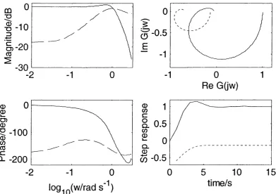
Figure 3-7: Bode plots of the sensitivity functions 80

Figure 3-8: Bode plots of the real process and the estimates 81

Figure 3-9: Nyquist plots and step responses of the real process and the estimates 81

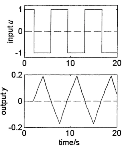
Figure 3-10: Relay feedback system 84

Figure 3-11: Limit Cycle from relay feedback 84

Figure 3-12: The amplitude-biased relay 89

Figure 3-13: Oscillatory waveforms under amplitude-biased relay feedback 89

Figure 3-14: Relay feedback system with Butterworth filter 93

Figure 3-15: Frequency response of a typical Butterworth filter 94

Figure 3-16: Time trends for the DF2 method 96

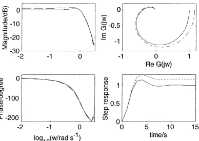
Figure 3-17: Nyquist plots of the real process and estimate from DF2 method 98

Figure 3-18: Time trends by using the TD l method 99

(14)

Figure 3-22: Nyquist plots of the three estimates with the real process 102

Figure 3-23: Identification errors of the three methods 102

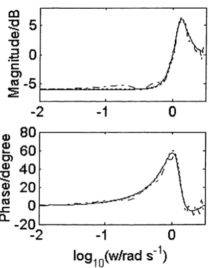
Figure 3-24: Time trends for the test with white noise disturbance 103

Figure 3-25: Measurement Noise Influence of FFTl method 104

Figure 3-26: Information identified by different methods 105

Figure 3-27: Time trend and probability density function for the process inputs 109 Figure 3-28: Comparison of identification results and the worst case error 112

Figure 4-1 : Continuous/sampled, analogue/quantized signals 118

Figure 4-2: The mid-rise quantizer and the mid-step quantizer 119

Figure 4-3: The quantizer in Matlab Simulink 120

Figure 4-4: The quantizer used in this thesis 121

Figure 4-5: the example for quantization error study 122

Figure 4-6: The unquantized signal, quantized signal and the quantization error 122 Figure 4-7: Spectral characteristics of the quantization error plotted in Figure 4-6 123

Figure 4-8: Quantizer inserted in the feedback path 125

Figure 4-9: CLID methods suitable for different quantization interval {qi) 125 Figure 4-10: The relationships of the signal-to-noise ratio with qi for the given process and

that of the correlation of the quantizer excitation and disturbance with qi. 128 Figure 4-11: Quantizer input, output and quantization error in time and frequency domain 129 Figure 4-12: Influence of the hysteresis width and relay amplitude in relay identification 131

Figure 4-13: Normal distribution theory 132

Figure 4-14: Scheme of CLID with a quantizer 133

Figure 4-15: CLID methods suitable for different quantization interval {qi) 134 Figure 4-16: Stability analysis after inserting a relay with hysteresis 135

Figure 5-1 Closed-loop system with excitation in the forth ward path 137

Figure 5-2 Closed-loop system with excitation in the feedback path 138

Figure 5-3 The proposed CLID with a quantizer scheme 140

Figure 5-4 Scheme of relay-based identification with quantizer 143

(15)

Figure 5-10 Simulation for CLID with a quantizer for the temperature loop 152 Figure 5-11 Simulation for relay identification with a quantization for temperature loop 153 Figure 5-12 Experimentation for CLID with a quantizer for temperature loop 154

Figure 6-1 Simulation for CLID with a quantizer 156

Figure 6-2 The relationships of the signal-to-noise ratio with qi for the given process and that of the correlation of the quantizer excitation and disturbance with qi. 157 Figure 6-3 Quantizer input, output and quantization error in time and frequency domain 158 Figure 6-4 The relationships of the signal-to-noise ratio and correlation change with qi for

different controllers 160

Figure 6-5 CLPA index for proportional controller with different Gain 160

Figure 6-6 Result for simulations shown in Table 5.2 162

Figure 6-7 Result for C U D with a quantizer for the continuous transfer function 163 Figure 6-8 Result of relay-based identification with a quantizer for the continuous

transfer function process 164

Figure 6-9 The open loop identification results of the simulated temperature loop 165 Figure 6-10 Results for CLID with a quantizer for the simulated temperature loop 167 Figure 6-11 Result of relay-based identification with a quantizer for the simulated

temperature loop 168

Figure 6-12 The open loop identification results of the temperature loop by experiment 169 Figure 6-13 Results for CLID with a quantizer for temperature loop by hybrid experiment 170 Figure 6-14 Results for CLID with a quantizer for temperature loop by natural bubble

experiment 171

Figure 7-1 Model order determination for a sine wave with quantization interval 0.5 189

Figure 7-2 Reconstruction of a sine wave from quantized samples 192

Figure 7-3 Reconstruction performance for a sine wave from quantized samples 193

Figure 7-4 Reconstmction of quantized plant data 195

(16)

Table 3.1 Different signal to noise ratio conditions 71 Table 3.2 Results duplicated vs results published in Li. et al. (1991) 97

Table 4.1 Nonlinearity index for unquantized and quantized signals 124

Table 5.1 CLID with a quantizer for different controllers 146

Table 5.2 CLID with a quantizer simulation conditions for discrete model simulation 147 Table 5.3 CLID with a quantizer simulation conditions for pilot plant model simulation 152

Table 6.1 Results corresponding to simulations of Table 5.1 159

Table 6.2 Worst case errors for identified models corresponding to simulations Table 5.2 161

Table 6.3 Nonlinearity index for unquantized and quantized signals 164

Table 6.4 Conditions corresponding to simulation results in Figure 6-10 166

Table 6.5 Summary of simulations and experimentations 173

Table 7.1 Test Results for the influence of ensemble length 190

(17)

The nomenclature follows Soderstrom & Stoica (1989) and/or Ljung (1987)

è : an estimate : the true value

E è : E is the expectation operation

N: the number of data points used in the estimate : the data set

M: Model Structure

G ; an estimate of the true process Go Go : the true process

C: the controller

d : the relay amplitude in the context of relay-based identification

d { t) : the external excitation in the context of closed loop identification with external excita tion.

a : the amplitude of the oscillation in the process output (limit cycle) in the context of relay- based identification

a{t) : the noise in the context of closed loop identification with external excitation

K\ the process steady-state gain L: the dead time

T: the time constant

s: Laplace variable

qi: quantization interval

ql: quantization level

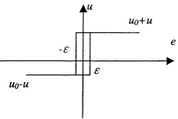
h : quantizer output amplitude e: hysteresis width

u : process input

y: the process output

(18)

CHAPTER 1 INTRODUCTION

This chapter begins by presenting an overview, followed by the important definitions and concepts in system identification and closed-loop system identification. The objective and the motivation of this thesis and the key issues to be addressed are described. The last sections give the outline of the approaches used throughout this thesis and the organization of the thesis.

1.1 O verview

1.1.1 A n exam ple

The closed loop control system is common in everyday life, for example a hot water tank in a domestic house. In this example, the hot water tank is the controlled system because it is desired to maintain the hot water at a desired temperature by means of a heating element. The tank and the heater comprise a closed loop. There are generally two ways to find the model of a system. One way is through application of the laws of physics. The other way is by system identification. For the hot tank example, the first possible approach is to calculate the model after knowing the size of the tank, the heat transfer rates and so on. Another is to infer the model from measurements of the heat input and temperature over a period of time. Closed-loop identification uses the latter method. Closed-loop identification is a challenge because the aim of the control system is to keep the temperature constant, yet identification requires the temperature to change in order to give some information about the tank.

1.1.2 M otivation

This thesis aims to find novel ways to meet the challenges involved in closed-loop identification. For the hot tank example, on the one hand, the system must be disturbed, for instance, by switching the heater on and off. On the other hand, the disturbance must be minimized in order to maintain the temperature at the correct value. Therefore the motivation of the work is to find a means of supplying sufficient information with a minimum of disturbance.

(19)

excite the identified process. Therefore, the aim of this thesis is to find the dynamics of a controlled system from closed-loop quantized data.

1.2 D efin ition s a n d con cepts

This section will first give some basic definitions on system identification. Closed-loop identification will then be discussed. Emphasis will be given to two specific closed-loop identification methods — closed-loop identification with external excitation and relay-based identification.

1.2.1 Basic definitions

The focus of the work is the determination of the behavior of controlled system, while it remains under closed loop control. The Instrument Society of America gives the following definitions.

Controlled system: The collective functions performed in and by the equipment in which the variable(s) is (are) to be controlled.

(ANSI/IS A -S51.1 -1979:29)

Closed loop: A signal path, which includes a forward path, a feedback path and a summing point, and forms a closed circuit.

(ANSMSA-S51.1-1979:8)

Feedback control: Control in which a measured variable is compared to its desired value to produce an actuating error signal which is acted upon in such a way as to reduce the magnitude of the error,

(ANSI/ISA-S51.1-1979:11)

For the hot tank example, the hot water tank is a controlled system because it is desired to maintain the hot water at a desired temperature by means of a heating element. The tank and the heater comprise a closed loop.

1.2.2 System identification definitions

When a new system is encountered, some concept of how its variables relate to each other is needed. With a broad definition, such an assumed relationship among observed signals is a

(20)

be described by their impulse or step responses. These are graphical models. In more advanced applications, it may be necessary to use models that describe the relationships among the system variables in terms of mathematical expressions like difference or differential equations. These are mathematical (or analytical) models. Mathematical models may be further classified into different types, such as continuous time or discrete time, lumped or distributed, linear or nonlinear. Throughout this thesis, only mathematical models of linear lumped systems will be discussed.

This subsection now introduces some basic concepts that will be valuable when describing and analyzing identification methods (see, for example, Ljung, 1987; Soderstrom and Stoica, 1989).

Process and svstem:

The physical reality that provides the experimental data will be generally referred to as the process. ... The word system denotes a mathematical description of the true process.

(Soderstrom and Stoica, 1989:9)

In Figure 1-1, the true process is Gq . For instance, if expressed as continuous linear system, it may take the form of

where G(5) is the transfer function, K is the process steady-state gain, L is the dead time, T is the time constant and s is Laplace variable.

Svstem identification:

System identification is the field of modeling dynamic systems from experimental data.

(21)

(1.2)

Where u is the input and y is the output. The task of system identification is to determine an estimate G of the true process Gq from the data set Z ^ . Still for the hot water tank in a domestic house, the behavior to be identified is the relationship between tank temperature and heater input, e.g. how much heat is needed to raise the temperature by 1°C (the gain) and how long it takes for the tank to attain some fraction of the desired temperature (63% is commonly used).

Ho

Go

F igure 1-1 Open-loop system in which Gq is the true process and Hq is the noise

model; a is white noise and v is the noise applied on the process.

Nonparametric methods: A model that is described by a curve, function or table is called a

nonparametric model. A step response, an impulse response and a frequency diagram such as Bode and Nyquist plots are examples of nonparametric models. Methods that aim at determining nonparametric models by direct techniques without first selecting a confined set of possible models, are often called nonparametric methods since they do not (explicitly) employ a finite-dimensional parameter vector in the search for a best description.

In system identification, commonly used nonparametric methods include, for example, the correlation analysis method and the spectral analysis method (Ljung, 1987).

Model Structure M:

(22)

model will be denoted H( 0) . When Û is varied over some set of feasible values, we obtain a model set (a set of models) or a model structure M.

A general parametric model structure (Ljung, 1991) is

A { q ) y i t ) = - nk) + ^ ^ e { t ) (1.3)

F{ q) D{q)

where A,B,C,D and F are polynomials in the delay operator q'^:

A{q) = 1 + + ... (1.4)

B{q) = b^q~^+...(L5)

C (^ ) = l + c , g " '+ ...(1.6)

D{q) = \-¥d,q-^ +...(1.7)

F ( ^ ) = l + / , ^ - ' + ... (1.8)

in which, n^, and are the orders of the polynomials A,B,C,D and F, k is the number of delays from input to output.

Other linear parametric models are special cases of the above general parametric model structure. For example, the general parametric model structure becomes an ARMAX model when both and equal to zero.

(23)

The general parametric model structure becomes Box-Jenkins (BJ) model when equals to zero.

y{t) = u{t - nk) + e{t) (1.10)

F ( ^ ) D (^)

ARX model is another special case of the general parametric model structure when and

My all equal to zero.

M q ) y ( t ) = B{q)u{t - nk) + e{t) (1.11)

In the special case of ARX model where n^ = 0, ARX model becomes FIR (finite impulse response) model.

y( t) = B ( q ) u ( t - n k ) + e{t) (1.12)

Parameter estimation methods: When a set of candidate models has been selected and it is parametrized as a model structure using a parameter vector 6, the search for the best model within the set then becomes a problem of determining or estimating 0 . If the data set has been collected, then the definition is as follows:

The problem we are faced with is to decide upon how to use the information contained in to select a proper value 0/^ of the parameter vector, and hence a proper member M (^yy ) in the set M *.

Formally speaking, we have to determine a mapping from the data Z ^ to the set (set of values over which 0 ranges in a model structure

M)

Z " - ê , (1.13)

Such a mapping is parameter estimation method.

(24)

In system identification, commonly used parametric methods include, for example, the least- squares (LS) method and the maximum likelihood (ML) method.

Bias: When the expected value of an estimate 6 deviates from the true value , i.e. E Ô ^ Oq,

where E is the expectation operation, the estimate $ is biased. The difference E O -Oq '\^ called the bias. Otherwise, if E 9 = 0q, 0 is said to be unbiased. (Soderstrom and Stoica, 1989:18)

Consistencv: An estimate Ô is consistent if ^ as N-*oo, where N is the number of data points used in the estimate. A reasonable altanative is ‘limit with probability one’ (Soderstrom and Stoica, 1989:19).

Identifiabilitv: This is a concept that is central in identification problems. Loosely speaking, identifiability is whether the identification procedure will yield a unique value of the parameter

6 and whether the resulting model is equal to the true system The issue involves aspects on whether the data set Z ^ is infcrmative enough to distinguish between different models as well as whether different values of 6 can give equal models (Ljung, 1987:99). Generally, the term system identifiability refers to the joint identifiability of the process Gq and the

disturbance/noise model ffo (a s shown in Figure 1-1). Howeva:, throughout this thesis, only

the identifiability of the process Gq is concerned because only the true process is of interest.

Persistent exciting: This is an important concept which will be used repeatedly in this thesis.

A quasi-stationary signal [u(t)} with spectrum (p„(0)) is said to be persistently exciting if

<^,(6>)>0, Vû; (1.14)

(Ljung, 1987:364)

1.2.3 Closed-loop identification (CLID)

(25)

Closed-loop Identification is the procedure of collecting experimental data from a process while it is operating under feedback control and then using those data to develop a dynamical model for the system.

(MacGregor and Fogal, 1995:163)

A large number of academic papers on the topic of closed-loop identification (CLID) have been published. There are three main categories of closed-loop identification.

#

The first category is the general identification technique for stochastic processes. The process input is usually an independent, persistently exciting signal (i.e. a broad-band excitation signal that excites the process at many frequencies). The identification result is usually a discrete-time model, for example (Ljung, 1987)

G (9 ) = 9 - ‘ 4 ^ (1.14)

A{q)

where G(q) is pulse transfer function, B and A are polynomials, q \s forw ard shift operator,

correspondingly q'^ is backward shift operator and k is the number of delays from input to output.

This identification result can then be used for model-based control design. The typical overview papers on this topic are Gustavsson et a l (1977) and Forssell and Ljung (1999).

The second category occurs in the context of auto-tuning. It is an alternative to the Ziegler- Nichols frequency response method. A nonlinear relay is connected to replace the available controller. No input signal is used in this method. The final identification result is usually a continuous model, or transfer function, for example (Âstrôm and Hagglund, 1995)

Ke~^'

G( s) = - ~ (1.15)

i J + l

(26)

This continuous model is then used for Proportional-Integral-Derivative (PID) controller tuning. The well-known work is Âstrôm and Hagglund (1984a). This is called Relay-based identification.

In the third category, a step or pulse is used as process input signal. The end product is also a continuous model, which is consequently used for PID controller tuning. For example, Yuwana and Seborg (1982) proposed the estimation of the critical point of the process (i.e. where its frequency response has a phase shift of 180°) based on a first-order plus dead time (FOPDT) model identified from a step set-point response of the proportional control system. This is called a proportional (P) controller method.

In the literature, when closed-loop identification is referred to, it always means the first category by default. For easy notation so as to avoid confusion, the first category is called

closed-loop identification with external excitation in this thesis since an independent persistently exciting signal (i.e. a broad-band excitation signal that excites the process at many frequencies) is used to guarantee closed-loop identifiability in all the methods of this category. The second category is called relay-based identification. In this thesis, only the first two categories will be studied in detail since they will be further developed to formulate a new closed-loop identification scheme.

1.2.4 C losed-loop identification with external excitation

External excitation is a dither signal injected into the original closed-loop system to excite the process for the purpose of system identification. A single-input single-output (SISO) closed- loop system (adopted from MacGregor and Fogal, 1995) illustrated the material to be presented in this subsection. It provides a general structure for CLID with external excitation. The excitation is a dither signal introduced at d.

In Figure 1-2, G^ iq) represents the true process, and the disturbance v{t) = HQ{q)a(t)

(27)

The identification task is to use y(t) and d(t) to identify the process. This can be done in a number of ways, for example, Huang and Shah (1997), Van den H of and Schrama (1993).

ysp

Ho

Go

F igure 1-2 Closed-loop system

1.2.5 R elay-based identification

In normal condition, the process works under the control o f a controller (Figure 1-3). The idea was to introduce a nonlinear feedback of the ideal relay in order to generate a sustained oscillation during the identification. The system then starts to oscillate. The period and the amplitude of the oscillation are determined when steady-state oscillation is obtained (Âstrôm and Hagglund, 1995). The measured oscillation information can be used in two ways, either to estimate the critical point of the process, that is where its frequency response has a phase shift of 180° and thus may be regarded as an automated Ziegler-Nichols test.

ysp

Go

(28)

1.3 Problem analysis a n d key issues

1.3.1 Problem analysis

At this moment, a natural question raised often is that: With so many choices for closed-loop identification methods, why are new schemes for closed-loop identification still needed?

Within the first category, CLID methods rely on external perturbations to excite the process. These perturbations, such as adding a dithering signal to the control loop, are not a part of the closed-loop and are external to the process under feedback control. The role of these signals is to excite the process for the purpose of identifying the true dynamics of the process while the process is operating under feedback control. This excitation has the unfortunate effect of degrading the control performance because it is an external disruption to the process. It cannot be avoided, but should be minimized.

On the other hand, as described in subsection 1.2.5, information on the critical point can be identified from relay feedback tests. These parameters allow PID tuning settings to be calculated, for instance from Ziegler-Nichols rules or other standard tuning methods. Relay tuning has been successful. For example, the Alfa Laval Automation ECA400 controller that is commercially available is based on relay identification (Âstrôm and Hagglund, 1995). However, the problem is that replacement of the PID controller by the relay disrupts the operation of the control loop.

Achieving identification during normal operations without external excitation or disruption is an ideal target. But theoretical analysis and simulation studies for closed-loop identifiability in section 3.1 will show that it is impossible. So the best solution should identify the process dynamics with as small disruption to the controlled process as possible.

The observation that quantization caused by analogue to digital (A/D) conversion and/or digital to analogue (D/A) conversion in the process instruments injects an excitation into a single input-single-output (SISO) loop even during normal process operations should be inspiring (EPSRC Grant Proposal GR/R06687 by Thornhill et a l 2000).

(29)

y - y „ in Figure 1-4) acts as the excitation. The 10-bit A/D converter for measurement purpose is not very flexible. Therefore, the last scheme should be like that displayed in Figure 1-5 with another A/D converter inserted in the feedback path. The excitation can be adjusted in two ways, either by increasing the quantization interval of the additional A/D converter, or by altering the quantization sampling rate (i.e. the times at which the quantized samples are taken) of the additional A/D converter. The quantization error ( y ^ - y in Figure 1-5) will be used as the excitation required by closed loop identification.

ysp

Go A / D

Figure 1-4 Closed-loop system with 10-bit A/D converter

ysp

Go A /D

A /D

Figure 1-5 Closed-loop identification using quantized data

It is the aim of this thesis to find novel ways to meet the challenge of achieving identification during normal operations with minimum disturbance. Quantizer signal processing seems to be a potential solution. Therefore, the motivation of the work is to find how to use the quantizer to excite sufficient information for system identification while minimizing the disturbance.

1.3.2 K ey issues

(30)

disruption to the controlled process. The key idea is to exploit measurement quantization errors caused by analogue to digital conversion as an excitation signal.

To achieve the target described above, the following key issues need to be addressed.

• To explore the different ways that can meet closed-loop identifiability. This will provide theoretical fundamentals why closed-loop identification can be achieved based on quantization.

• To compare the advantages and disadvantages of the CLID with external excitation method and the relay-based identification.

• To recover an underlying signal from quantized measurements. The quantization error is the quantized observation minus the unquantized/underlying signal. After the quantized data has been obtained, the key issue is to implement an algorithm to recover the underlying signal.

• To explore the relationship between quantization interval and the information content of quantization error. This information content includes power and bandwidth.

• To select the optimum quantization interval or range for different closed-loop identification methods.

• To formulate new CLID scheme for controlled system identification using quantized data. • To demonstrate accurate system identification using quantized plant data with pilot plant

experimentation

1.4 O utline o f approaches

1.4.1 C ase study

Case studies will be extensively used to validate theory and to gain insights for different closed- loop identification methods. In section 3.1, case studies will be used to validate the theory on closed-loop identifiability. Then in section 3.2, case studies will be used to duplicate the two- stage method (Van den Hof and Schrama, 1993) and the two-step method (Huang and Shah, 1997). In the same way, the relay identification methods (Li. et a l, 1991; Wang, QG et a l,

(31)

1.4.2 Sim ulation

Simulation is widely used to test the theory and the algorithms. In Chapter 3, all case studies will be implemented through simulation. In Chapter 5 and Chapter 6, transfer function model simulation and pilot-plant model simulation will be used to demonstrate the closed-loop identification scheme based on quantization. In Chapter 7, simulation will be used to demonstrate the superiority of Quantized Regression (QR) algorithm over other methods (e.g. the Linear Least Square (LLS) method) in reconstructing from quantized measurements.

All the simulation analyses were performed using MATLAB version 6.0 together with Simulink version 4.0 and System Identification Toolbox version 5.0 (The Math Works; Natwick, MA).

1.4.3 Experim entation

Experimentation is a convincing way to test the theory and the algorithms. In Chapter 5 and Chapter 6, experimentation with a pilot plant in the Computer Process Control group in the University of Alberta will be used to demonstrate the closed-loop identification scheme based on quantization. In Chapter 7, experimentation data of the pH control in a buffered fed-batch yeast fermentation process will be used to demonstrate the superiority of quantized regression (QR) algorithm over other methods (for example, the linear least square (LLS) method) in recovering the underlying signal from quantized measurements.

1.5 O utline o f th e thesis

In this thesis, the general objective is described in Chapter 1 on the basis of introducing the important definitions and concepts as well as two main categories of closed-loop identification methods: closed-loop identification with external excitation and relay-based identification. Emphases are put on the problem analysis and key issue to be addressed. Chapter 2 is a literature review in which the developments of the two categories of identification methods and the relevant closed-loop identification based on quantization are evaluated. The topic of closed- loop performance assessment (CLPA) is also reviewed since the concept and method will be further used in Chapter 5 and Chapter 6.

(32)

presented in Chapter 3. The main advantage for relay-based identification is that the sustained oscillation can be implemented automatically. The main disadvantage for relay-based identification is that the controller must be replaced by an ideal relay, which means disruption to the control system. The main advantage for closed-loop identification with external excitation is that over a range of frequencies information of the process can be identified and the identified model is of higher accuracy. The main disadvantage for closed-loop identification with external excitation is that a priori information on the critical frequency of the identified system is needed for the design of the persistently exciting signal. These case studies will also provide a benchmark for further work of assessing the new closed-loop identification schemes.

Chapter 4 starts with the definition of quantizers. The relationship between quantization interval and the information content (power and bandwidth) of the quantization error is then presented. A new closed-loop identification scheme is proposed - when quantization interval ranges from small to large, the closed-loop identification with external excitation method and the relay-based identification method can be applied correspondingly. The stability influence of the newly inserted quantizer to the closed-loop system is also analyzed in Chapter 4. Chapter 5 introduces the computation methods such as a nonlinear test method, model accuracy measure, the simulation method and the experimentation method. All the results and discussions are written in detail in Chapter 6.

Chapter 7 is a self-contained chapter, which presents the Quantized Regression (QR) algorithm used to recover the underlying signal from quantized measurements. The QR algorithm was implemented successfully but was not in the end used in the closed-loop identification procedure because its large computation makes it difficult to use on-line.

(33)

CHAPTER 2 LITERATURE REVIEW

This chapter focuses on closed-loop identification with external excitation (Ljung, 1987) and relay-based identification (Âstrôm and Hagglund, 1984a and 1984b). It also includes some previous research on closed-loop identification with a quantizer. The relevant topic of closed- loop performance assessment (Harris, 1989) is also discussed since it will be used later in Chapter 4, Chapter 5 and Chapter 6 of this thesis.

2.1 C losed-loop identification with external excitation

In this section, a general structure for closed-loop identification with external excitation will be described first. The efforts will then be directed to classification and development of the CLID approaches and methods. The recent development of closed-loop identification without external excitation is also discussed. The conclusion is given in the end that some kind of external excitation is necessary for closed-loop identification.

2.1.1 Introduction

The single-input single-output (SISO) closed-loop system (adapted from Ljung, 1987) illustrates the material to be presented in this section. It provides a general structure for CLID with external excitation. The excitation is a dither signal introduced at d.

ysp

Go

Ho

F igure 2-1 Closed-loop system

The true system is assumed to be

(34)

where G ^ iq ) represents the true process, and the disturbance v{t) = / / q ( ^ ) û ( 0 represents the effect of all unmeasured process disturbances on the measured output y(t), q is the forward shift operator. The feedback loop is

u{t) = C{q){y^p (t) - y (t)) + d ( t) (2.2)

where C(q) is the feedback controller, and the set-point y,p{t) and the ‘dither’ signal d(t) are input signals that may be injected to aid in the identification. As stated in subsection 1.2.4, only

y^p(t) = 0 is considered in this thesis. Thus, the task of identification is how to use the available information (such as d(t), u(t) and y(t) ) to get an estimate G of the true process Gq . 2.1.2 M otivation

Closed-loop identification (CLID) identifies a process model while the process is operating under feedback control. Closed-loop identification might be necessary because the system is unstable in open loop or the system contains inherent feedback mechanisms (Ljung, 1987).

Gustavsson et a l (1977) gave an overview of CLID mainly on closed loop identifiability and accuracy. Their conclusions are that prediction error methods can be applied to identify linear model using data collected in a closed-loop and identification is possible in some cases, for example, external excitation, setpoint change, time-varying controller or nonlinear controller. Forssell and Ljung (1999) revisited CLID under the prediction error framework. Van den Hof and Schrama (1995) systematically reviewed the problem of control-relevant CLID. Their main conclusion is that iterative closed-loop identification and control design can improve performance.

2.1.3 Fram ew ork o f approaches and m ethods

Different assumptions of feedback configurations lead to a classification of CLID approaches (Gustavsson et a i, 1977; Forssell and Ljung, 1999):

(1) The Direct Approach: the feedback is ignored and the controlled system is identified using measurements of the input u(t) and the output y(r) (see Figure 2-1).

(35)

(3) The Joint Input-output Approach: the input u(t) and the output y(t) are jointly viewed as the output from a system driven by the external excitation signal d(t) and noise a(t). Some method is used to determine the open-loop parameters from an estimate of this augmented system. It is not required to know the controller C(q), but the controller must be known to have a certain structure. In detail, three branches exist inside Joint Input-Output Approach (Gustavsson et a l, 1977; Forssell and Ljung, 1999). They are: the Coprime Factor method, the Two-stage (step) method, and the Projection method.

Thus, the framework for CLID with External Excitation is: • Direct approach

• Indirect approach

• Joint input-output approach • Coprime factor method

Coprime factors means having no common factors (Schrama, 1991). • Two-stage (step) method

There are two stages or steps; the first stage/step is to identify sensitivity function and the second stage/step is to identify the process model (Van den Hof and Schrama, 1993; Huang and Shah, 1997).

• Projection method

This method is similar to two-stage/step method, the difference is a non- causal FIR filter used in the first sage/step; the first step in the method can be viewed a least squares projection of the process input u(t) onto external excitation d(t) - hence it is called projection method (Forssell and Ljung,

1998; Forssell and Ljung, 1999).

On the other hand, in the context of open-loop system identification, the textbook of Ljung (1987) classifies open-loop system identification into

• Parametric method

With this method, a model structure (finite dimensional parametric vector) has to be chosen at first, followed by parameter estimate and model validation.

• Prediction Error family

(36)

• Least square method, in which the estimate is obtained by choosing the criterion as minimizing the sum of the squared one-step-ahead prediction errors, it is also called linear regressions in the literature; it is a special case of

prediction error identification methods (Ljung, 1987: 175-176).

• Instrumental Variable method: the key difference between IV methods and LS methods is that LS methods can only be used when the measurements are contaminated by white noise and IV methods can be used under coloured noise for consistent estimation (Soderstrom and Stoica, 1989, ppI87, pp26I; Ljung,

1987, ppI92-I93). • Subspace family

Subspace methods estimate a state space model of a multivariable process directly from input/output data. The main part of a subspace method consists of matrix singular value decomposition (SVD) and linear least-squares estimation which are numerically simple and reliable (Zhu and Butoyi, 2002).

• Non-parametric method

A model is described by a curve (for example, impulse response, step response), a function or a table; a finite-dimensional parameter vector is not explicitly employed in the search for a best description (Ljung, 1987, ppl4I).

• Correlation method in which the input is white (if it is not white, a whitening filter can be used to make it white), the impulse response can be calculated through correlation analysis (i.e. the cross covariance function between the input and the output) (Ljung, 1991, ppl-17).

• Spectral analysis method in which the frequency response is obtained by dividing the cross spectrum of the output and the input with the spectrum of the input (Ljung, 1991, ppl-18).

(37)

2.1.4 Specific approaches and m ethods

In this subsection, different methods will be placed in the context of the approach used. The aim is to make the classification in section 2.1.3 more concrete to present the methods that have potential use in the thesis later.

Direct approach

The direct approach can only be used with the prediction error method and some of the subspace methods. The reason for this is the unavoidable correlation between the unmeasurable noise and the input.

Indirect approach

Theoretical analysis reveals that application of the conventional least-squares (LS) method in indirect identification can always result in inconsistent parameter estimates of the closed-loop system as well as of the open-loop process in the presence of coloured noise. Zheng and Feng (1995) presented an LS type method to cope with the bias problem in indirect identification of closed-loop systems subjected to coloured disturbances. The proposed method is based on the bias-correction principle. The suggested method can yield consistent parameter estimates. Generally, this kind of method is referred to as bias-free least squares (BFLS).

The instrumental variable (IV) methods form a different class of identification methods that is related, but not equivalent, to the least square (LS) methods inside the prediction error framework. The key differences between IV methods and LS methods are that LS methods can only be used when the measurements are contaminated by white noise and IV methods can be used under coloured noise for consistent estimation (Soderstrom and Stoica, 1989, ppl87, pp261). The closed-loop IV methods have been studied by Soderstrom et al. (1987). Under weak assumptions, the estimates are consistent and asymptotically Gaussian distributed. To guarantee the identifiability of the closed-loop, a measurable external signal such as a reference or a setpoint is needed.

(38)

Joint inout-output approach

Schrama (1991) proposed a framework for open-loop identification of the coprime factors of the unknown plant in dealing with the approximate closed-loop identification problem. This framework allows the feedback-controlled plant to be identified by the application of any open- loop identification method.

Van den Hof and Schrama (1993) introduced a two-stage method. The transfer function of a linear plant can be consistently estimated on the basis of data collected from closed loop experiments, even in the situation where the model of the noise disturbance is not accurate. Huang and Shah (1997) modified the two-stage method described above and demonstrated better accuracy. Both researches require that a persistently exciting external signal (i.e. a broad-band excitation signal that excites the process at many frequencies). Esmaili et al. (2000) discussed the asymptotic and finite data behaviour of some closed-loop identification methods including the two-step method (Huang and Shah, 1997).

Forssell and Ljung (1998) initiated a projection method, which comprises the same two steps as the two-stage or two-step method. The only difference is that in the first step one should use a non-causal FIR model instead of a causal high-order FIR or ARX model.

ARX model is a commonly used parametric model, for example

= = (2-3)

A{q) A{q)

where B and A are polynomials in the delay operator q ':

A{q) = \ + a^q ' + ... (2.4) % ) = l + 6 , ^ - ' + ...(2.5)

(39)

M 2

u{t) = S { q ,P ) d { t) + e {t)= + (2.6)

k = ~ M I

where M l and M 2 are positive integers and d is the input. The main feature is that the sum contains both the positive items and the negative items - which means past and future.

2.1.5 C losed-loop identifiability, accuracy and efficiency

The issues of identifiability, accuracy and efficiency were important topics in the early stages of closed-loop identification in 1960s and 1970s. They remain under investigation in the literature.

Closed-looD identifiabilitv

Gustavsson et al. (1977) is the most widely referred paper on closed-loop identifiability. MacGregor and Fogal (1995) discussed the closed-loop identifiability with simulation examples. They showed that the nonparametric methods yield no information on the true system if data from purely feedback operation is used. Under the same condition, the parametric methods can identify the true system only when the fairly strict necessary and sufficient conditions on the true process and controller orders are satisfied (i.e. order of the controller should be greater than, at least equal to, the order of the process). In Gustavsson et al.

(1977), this is called system identifiability (SI).

It is apparent that for closed-loop identification something must be done to break the dependency between the input signal and the process disturbance. This can be accomplished in either of the two ways (MacGregor and Fogal, 1995; Bartee and McFarlane, 1998).

(1) By injecting an independent, persistently exciting signal into the feedback loop. (2) By switching between two or more feedback controllers.

Either of these will guarantee that necessary and sufficient conditions for identifiability be satisfied. This is known as strong system identifiabilty (SSI) (Gustavsson et a l, 1977).

The third way to break the dependency between the input signal and the process disturbance is to insert nonlinearity (page 366 of Ljung, 1987). For instance, switching between two or more feedback controllers is one way to implement nonlinearity.

SSI infers the following properties (Gustavsson et a l, 1977):

(40)

(2)A11 statistical estimation methods (non parametric method and parametric method) and validation techniques are valid.

(3)Descriptive transfer function models can be identified, even when they are over parameterized.

Therefore injecting external excitation into a system makes it to be SSI. The injection of an independent signal into the loop provides the user with a greater flexibility for designing the identification experiment to achieve the desired objectives. That is why this category is called closed-loop identification with external excitation.

Accuracv

The problem of assessing the quality of the estimated model, i.e. the accuracy, is an important issue in system identification (Gustavsson et a l, 1977). Model-plant error consists of two parts. One component is due to the fact that the true system is not within the model structure that has been chosen (e.g. under-modeling), and this is called the bias error. The second component of the total error is due to noise corruption of the observed data (disturbance effects or the random error). This is termed variance error.

The direct approach in which the feedback is ignored typically gives better accuracy than the indirect approach and joint input-output approach where the closed-loop problem is converted into an open-loop one. Ljung and Forssell (1997) derived variance results for a number of closed-loop identification methods using standard prediction eiror theory. By studying the asymptotic variance for the parameter vector estimates, they showed that indirect methods fail to give better accuracy than the direct method. So the direct approach should be regarded as the first choice of methods for closed-loop identification whenever possible. Gevers et al (2001) derived the asymptotic variance expressions for models that are identified on the basis of closed-loop data. The CLID methods considered include the direct method, as well as indirect methods such as coprime factorization method, dual Youla/Kucera parameterizations and the two-stage method by Van den Hof and Schrama (1993). They showed that different methods (direct method and indirect method) lead to the same asymptotic variance.

(41)

the consistency of the resulting model can be achieved without putting too much attention on the system disturbance model. For example, with the two-stage method proposed by Van den Hof and Schrama (1993), the transfer function of a linear plant can be consistently estimated even when the model of the noise disturbance is not accurate.

Ljung and Forssell (1999) studied the same problem i.e., direct identification of systems operating in closed-loop gives biased results whenever the true noise characteristics are not correctly modeled. When signal-to-noise ratio is large, the bias error will be small. But the only way to completely remove the bias is to use the indirect method.

Under certain circumstances, the instrumental variable (IV) method can give the same level of accuracy as the direct PE method. In general, though, the accuracy will be sub-optimal (Forssell and Chou, 1998). With optimally chosen instruments, the accuracy of IV method coincides with that of the direct method. However, this requires exact knowledge of the noise model and therefore cannot be achieved in practice.

Bias-free least squares (BFLS) method proposed by Zheng and Feng (1995) to cope with the bias problem in indirect identification of closed-loop systems subjected to coloured disturbances is based on the bias-correction principle. This might be useful in designing new closed-loop identification scheme with quantization signal processing.

Efficiencv

An unbiased estimate is said to be efficient if its covariance equals the Cramer-Rao bound.

(Norton, 1986:117)

(42)

2.1.6 Joint identification and control

From the 1990's, control relevant identification (or joint identification and control) has attracted much attention. The goal is to construct models that are suitable for control design. The key idea in the joint identification and control strategy is to identify and control with the objective of minimizing a joint global control performance criterion. Van den H of and Schrama (1995) reviewed the problem of joint identification and control. They discussed attempts to provide a separate analysis of both steps (approximate identification and model-based control design), and to accomplish a joint (robust) performance criterion o f both parts. The conclusion is that the latter can have better performance.

The study of control-relevant identification by Hjalmarsson et al, 1996 showed that the best identification strategy is to identify the process under feedback with the intended controller in use. Callafon (1998) studied the integration of closed loop identification with robust control design and the application of this method to manufacturing o f a wafer stage.

To perform dual roles of identification and control simultaneously within a constrained Model Predictive Control (MPC) framework is termed MPCI. Nikolaou and Eker (1998) introduced a new MPCI variant. Process inputs are constrainted to excite the process as much as possible for the generation of maximum parameter information. Gopaluni et al. (2002a and 2002b) also studied closed-loop identification with MPC controller as the intended controller. The conclusion is that it is important to minimize multi-step-ahead predictions, as opposed to one- step-ahead prediction errors, if MPC Controller is used. Zhu and Butoyi (2002) studied multivariable and closed-loop identification of industrial processes for use in MPC. Twu case studies were used to demonstrate the advantages of closed-loop identification.

2.1.7 T he problem o f C LID w ithout exctem al excitation

As described above, the paper of Gustavsson et al. (1977) showed that the injection of an independent signal into the loop guarantees the closed-loop identifiability. Generally, CLID methods rely on external perturbations to excite the process.

(43)

excitation has the unfortunate effect of degrading the control performance and should be minimized in some way.

Due to the above reason, researchers have been motivated by the desire to use only routine closed-loop operating data (i.e. without external excitation) for model identification. Sun et a l

(2001) proposed a new identification algorithm for a linear discrete-time closed-loop system. Identifiability condition was not satisfied because neither an external excitation was injected nor the controller was switched. The algorithm is based on output over-sampling scheme (i.e. output sampling interval is much smaller than input sampling interval). The over-sampled output data contain more information about the system structure. The restriction of the proposed method is that the model structure (including the order and delay time) o f the plant is assumed to be known. Bartee and McFarlane (1998) studied the identification of process models using routine operating data (or archived data) with simulation examples in a fluid catalytic cracking unit. They showed that with routine data (from systems satisfying SI), only when the true system structure is known, can an adequate model be identified. These publications showed that routine or archived data have limited practical use in closed-loop system identification. Therefore, there is a need for some kind of external excitation.

2.1.8 C onclusions

From the discussions in this section, the conclusions are:

• Closed-loop identifiability (MacGregor and Fogal, 1995) is an important topic.

• Van den H of and Schrama (1993) and Huang and Shah (1997) are all two-stage (step) methods of joint input-output approach, in which a persistently exciting external signal is needed. For the proposed project, the error between quantized measurements and unquantized measurements is equivalent to the external excitation. Thus the same procedures as in Van den Hof and Schrama (1993) and Huang and Shah (1997) can be used.

• Bartee and McFarlane (1998) discussed the use of routine operating data without external excitation for closed-loop identification with simulation examples. The conclusion is that archived data has limited use in closed-loop identification. Therefore, there is a need for some kind of external excitation.

(44)

2.2 R elay-based identification

In this section, the relay-based identification will be presented first, followed by the motivation. The emphasis will be placed on the development of relay-based identification schemes. The identifiability of the relay-based identification method, the noise issue and load disturbance impact, and the commercial products will also be briefly discussed.

2.2.1 Introduction

ysp

Figure 2-2 Relay feedback system