SHOCKS, PHYSICAL CHARACTERISTICS, AND RISK TAKING BEHAVIOUR
Muhammad Ryan SANJAYA 1 ABSTRACT
Many conventional economic analysis assumes that risk preference is taken as given and do not give much scrutiny on it. However, empirical studies show that risk preference is not random: shocks and predetermined characteristics can determine risk preference. This study tried to see if these potential determinants are together affect risk aversion in Indonesia using 2007 micro data. The author found that there is limited evidence that shocks and predetermined characteristics can affect risk preference. There is a preliminary indication that risk preference was not only driven by the individual’s wealth and demographic factors (that can be easily controlled), but also by the individual’s time preference.
Keywords: Risk aversion, Preference, Indonesia, Microeconometrics
INTRODUCTION
Many conventional economic analyses assume that risk preference is taken as given and do not give much scrutiny on it. In microeconomic theory, for example, a utility-maximiser individual is assumed to have a stable preference, either with regard to risk or non-risk preference. Otherwise, she will violate the axioms of consumer choice—especially the transitivity axiom—and analyses that are derived from this unstable preference will be inconsistent. In addition to that, risk preference is also thought to be one of the key ingredients in tastes formation, and tastes are mostly assumed as stable (Stigler and Becker, 1977). These arguments, however, does not suggest that stable preference should hold overtime. It means that an individual’s inconsistent behaviour can be attributed to random preference rather than unstable preference.
Nonetheless, some empirical studies suggest that risk preference is not random. For example, one of the most common assumptions when people are making decisions under uncertainty is that absolute risk aversion is decreasing with wealth (assuming that the Arrow-Pratt measure of absolute risk aversion is non-decreasing), which implies that individuals are willing to pay less for insurance if their wealth increases (Pratt, 1964)2. This assumption is proven empirically in lab experiment and in household survey as well (Guiso and Paiella, 2008; Holt and Laury, 2002).In addition to the role of wealth in determining risk aversion, several studies have found that shocks such as natural hazards make people less willing to take risk in disaster prone countries such as Peru, Nicaragua, and Indonesia (Cameron and Shah, 2011, Dang, 2012, van den Berg et al. 2009). Other than natural hazards, economic shocks can also have a positive relationship with risk aversion as observed from the effect of the 1930’s Great Depression on individual’s unwillingness to take financial risk (Malmendier and Nagel, 2011). These findings are psychologically intuitive: individuals update their information when there is an abrupt change (shocks) in their environment,
1
The author completed this paper during his postgraduate study at the Australian National University in 2012.
Email:[email protected] 2
Not only decreasing with wealth, but the shape of the curve is also important. See Figure A1 in the Appendix.
Asian Journal of Empirical Research
and this new information changes their risk behaviour. The question is, of course, if this relationship between shocks experienced and risk-taking attitude is consistent and perpetual.
Besides these shocks or temporary events, several studies argue that some predetermined characteristics such as genetic heritability can explain risk preference. Rubin and Paul (1979), for example, developed an evolutionary economics theory that links economic goods and ―inclusive fitness‖, a biological utility function that is maximised by the individual as a result of natural selection. This biological utility function ―punishes‖ individuals who are not willing to take risk in the form of having no offspring (genetically). Hence, this theory predicts that only those who are willing to take risk that will survive. This theoretical prediction is then developed by Ball et al.
(2010) by arguing that the taste for risk should co-evolve with superior physical prowess (and indeed they found that a physically stronger individual tend to be more risk loving).
This argument is also supported by a finding in the US that shows that twins who are not genetically identical tend to have lesser similarity in risk preference than genetically identical twins (Cesarini et al., 2009).Psychology can also explain the role of physical attributes. For example, taller people tend to get positive reinforcement from their environment and this translates into greater engagement in leadership role that required willingness to make risky choice (Korniotis and Kumar, 2012). Using data from the US and Europe, they found that taller people with normal weight are having greater likelihood to engage in the financial market and take risky portfolios. Across the Atlantic, in Germany, two studies also show that height could explain some of the variations in risk preference (Dohmen et al., 2009, Hübler, 2012). Another possible determinant of risk preference is parental education, in which the more educated parents tend to have children who are less risk averse (Dohmen et al., 2009;Hübler, 2012,Hryshko et al., 2011). This is probably because the more educated parents are, on average, having better knowledge about risk, and this knowledge is passed on to their child. However, it should be acknowledged that there is a likelihood that there are unobserved traits of the parent—other than their education achievement— that can explain children’s attitude toward risk.
Above studies on the determinant of risk aversion mainly relied on surveys and experiments conducted in developed countries where the populations are relatively homogenous. Using subjects from developing countries, on the other hand, is far more challenging yet interesting since the subjects are mostly constrained by income and, to some extent, are relatively heterogeneous. Indonesia, for example, is an interesting subject for studying the determinant of risk preference for it has more than 240 million people with wide array of diversity in its demographic, geographic and economic background. Therefore, this paper tried to answer the following question: do these potential determinants of risk preference significantly affect individual’s risk aversion in Indonesia?Cameron and Shah had done a study for Indonesia in 2011, but their contribution is limited to the impact of natural disaster on risk preference in rural area (especially East Java). This study took a wider look on any possible determinant of risk preference, which includes both the impact of shocks (such as natural disaster) and of individual’s predetermined characteristics (such as physical attributes and parental education), in both rural and urban area in Indonesia. While this result cannot be generalized over all countries in the world, but this study mostly contributes to the debates on risk taking behaviour in developing countries, especially a Muslim-populated countries, and its comprehensiveness in its analysis.
tend to choose low-earning job. However, if an individual’s risk preference is endogenously determined by wealth or income—as had been found in the regression results in this paper—then the estimated coefficients will be invalid. If this is the case, these studies might, for example, overestimate the impact of someone’s risk preference on occupational choice if we exclude the fact that the person just recently experienced natural disaster. With regard to the policy implication, one of the results from Cameron and Shah, (2011) study is that they suggest a policy that can increase the access for natural disaster related insurance. This follows from the finding that people who lived in villages that experienced disaster are more likely to engage in self-insurance. However, given the limited information outside East Java, this policy recommendation cannot be generalized for the whole Indonesia. Therefore this study adds to the debate on the importance of natural disaster insurance policy by taking a more general observation on Indonesia.
Data from the latest wave of the Indonesia Family Life Survey (IFLS4, 2007) were used as the main data source. The construction of risk aversion variable is not only following from previous studies but also from an alternative formulation that used all possible information from the survey. The main estimation method is OLS. If applicable, regressions were using subdistrict fixed effects and the standard errors were clustered at subdistrict level. Several sensitivity tests were conducted to ensure that the main finding is robust to variations in risk aversion measures. Subsample regressions were used as well to see how the relationship between risk aversion and its determinants varies among different sample group.
The preliminary result shows that, except for time preference and father’s education, only the usual demographic characteristics such as age, education, and sex that correlated with risk preference. Several subsample regressions resulted in the significance of height and disaster, but the pattern is scanty. There is also limited supporting evidence for disaster-related insurance promotion. The organisation of this study is as follow: Section 2 discussed data descriptions, variable constructions, and estimation methodology. Section 3 discussed estimation results, robustness checks, and a simple investigation on the policy implication. Finally, last section concludes.
ESTIMATION DESIGN
Data
Data from the Indonesian Family Life Survey (IFLS) were used to construct a measure of risk aversion. The IFLS was conducted by RAND cooperated with local research institutions in Indonesia and available for free at the RAND website3. While the respondents for the IFLS only come from 13 (out of 26) provinces in Indonesia but they represent around 83% of Indonesia due to the heavy population distribution in these selected provinces. The first wave of the IFLS was in 1993 and it has been repeated in 1997, 2000, and 2007.The IFLS consists of two blocks: household block and community block.
The household block measures individuals and household’s life such as consumptions, welfare, and health level, while the community block measures community/village life such as the availability of health facilities and school. Combined, there are 290 data files from these two blocks, each with specific information on the individual/household/community. While the IFLS is a panel dataset rich with information on households and individual’s behaviour, it is unfortunate that only in the latest available round (IFLS4) that it incorporates the questions on risk-taking behaviour. Nonetheless, I use information from IFLS2 (1997) and IFLS3 (2000) as well to construct several variables that I need in this essay.In addition to the IFLS, poverty rate data in 1996 and 1999 at district level were used as well in the sensitivity regression4
3
See http://www.rand.org/labor/FLS/IFLS.html 4
VARIABLE CONSTRUCTION
Risk aversion
In IFLS4 there are questions that can be used to measure risk aversion under the ―Risk and Time Preference‖ section. There are two games in this section, Game 1 and Game 2, in which they differ only in the amount of hypothetical money involved.5 In this section, the respondent will be asked to choose between two gamble and if he/she chose the risky one then he/she will move to the next question (which gives different payoffs).
In every question there is a ―Don’t Know‖ option that can be used to rule out respondent who do not understand the question6. Here’s an example of the gamble (see the Appendix for the full set of questions and description):
In Option 2 you have an equal chance of receiving either Rp1.6 million per month or Rp400 thousand per month, depending on how lucky you are. [On the other hand,] Option 1 guarantees you an income of Rp800 thousand per month. Which option will you choose?There are several methods that have been applied to construct risk aversion from the IFLS dataset:
1) Ordering based on the riskiness of the choice (Cipollone, 2011, Gaduh, 2012).
2) Binary variable, which simplifies risk choice into either risk loving or risk averse (Cameron and Shah, 2011).
3) Estimates the Arrow-Pratt index of Absolute Risk Aversion (ARA) (Permani, 2011).
By construction, Option 1) and 2) forced us to make two regressions based on Game 1 and Game 2. Option 2) is the simplest one in its construction, but it fits with Cameron and Shah experimental method since they do not use ordinal variable in the main part of their paper. Option 1) is capture more information on risk preference than Option 2) and will be used in the sensitivity analysis.By and large, Option 3) gives the best option due to the following reasons: first, ARA took information from both of Game 1 and Game 2.
Second, this measure is also linked directly with the theoretical underpinning of risk aversion (Pratt, 1964). Third, as can be seen in equation (1) below, ARA is a nonlinear, continuous variable that gives more variation in risk aversion. Therefore, I used ARA in the main regression where a higher value indicates a more risk-averse behaviour.ARA is constructed based on the expected utility of an individual’s participation in the gamble (after considering his/her initial wealth endowment as well).
5
This is probably the biggest drawback of using IFLS4 to construct risk aversion. With no stake involved, there is a chance that the respondent will choose randomly. However, IFLS is the most feasible dataset today in Indonesia that represents the largest population sample of Indonesia.
6
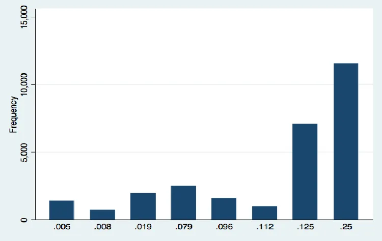
Figure 1: Absolute Risk Aversion frequency distribution
Table 1: Cross-correlations of various measure of risk aversion
ARA RL1 RL2
ARA 1.00
RL1 -0.51 1.00
RL2 -0.39 0.35 1.00
Table 2: Descriptive statistics
Variable Observations Mean Std. Dev
Measures of risk aversion
ARA 27717 0.15 0.09
RL1 27717 0.16 0.36
RL2 27717 0.05 0.22
Predetermined characteristics (PC)
Height (cm) 27717 155 12
Weight (kg) 27717 54 11
Ideal (=1) 27717 0.62 0.49
Tall (=1) 27717 0.49 0.50
Father’s education 27717 0.75 0.96
Mother’s education 27717 0.53 0.79
Temporary events (TE) Disaster (number disaster
experienced) 27717 0.15 1.70
Log of amount lost 27717 0.82 3.25
Log of assistance received 27717 0.57 2.71
Ecshock(=1 if in
construction/financial sector in 1997)
Variable Observations Mean Std. Dev
Change in poverty rate 27717 .58 .66
Ecshock ×
Change in poverty rate 8965 0.04 0.22
Other control variables (X)
Log of assets 27717 17.18 1.84
Log of past assets 27717 16.12 2.48
Muslim (=1) 27717 0.90 0.30
Javanese (=1) 27717 0.43 0.49
Rural (=1) 27717 0.48 0.50
Age (year) 27717 37 15
Male (=1) 27717 0.48 0.50
Married (=1) 27717 0.70 0.46
Dependency ratio (0-1, higher
more independent) 27717 0.36 0.23
Time preference (1-5, higher
more impatient) 27717 4.44 1.02
Education (0-4, higher
more educated) 27717 2.00 1.15
Cognitive ability (0-1, higher
smarter) 10642 0.74 0.24
Numerical ability (0-1, higher
smarter) 10642 0.42 0.31
Taking the second order Taylor expansion of the expected utility around the initial wealth endowment resulted in the following formula (where ZH is the high payoff (Rp1.6 million in the example above) and ZL is the low payoff (Rp400 thousand)):
ARA = ZH+ZL
ZL2+(ZH−ZL)2+ZL(ZH−ZL) (1)
From 10 questions on risk preference, the author found eight possible payoff combinations of ZH
and ZL that translated into eight values of ARA. The frequency distribution of ARA is skewed
toward those who are very risk averse (ARA = 0.25): 11,641 out of 27,717 observations (42%) are very risk-averse (with mean value of 0.15 and standard deviation of 0.09).In addition to this measure of risk aversion, we also used Cameron and Shah’s method (Option 2) and risk ordering (Option 1) in order to see how regression results change if we use different methods to measure risk aversion.With respect to the construction of risk aversion as described in Option 2), the author generates variable RL1 for Game 1 and RL2 for Game 2. RL1 and RL2 are binary variables that take the value of 1 if the respondent is risk loving. However, since these methods forced us to make two regressions based on Game 1 and Game 2 then we cannot really make a fair comparison with the main regression (that use information from both games to make a single regression).
necessarily completed) educational level. Moreover, around half of the parents were never been in school, which might be attributed to the fact that these uneducated parents were, on average, born around 1944 when Indonesia as a nation was not even born7.
Temporary events/shocks variables
I simply included the number of natural disaster experienced by the household, which comprises more than just earthquake and flood as in Cameron and Shah’s paper8. While there are data on the number of householder that was injured or killed because of the disaster but the variation is very small: more than 99% of the observation did not have their household member killed or injured due to the disaster. Including this in the regression will lead to large standard errors.IFLS also reports the amount of household’s belongings (business and non-business related belongings) that was lost due to the disaster. Many of the disaster victims also received financial assistance. I took the natural log of these and included as additional control variables.
Other control variables
The construction of other control variables such as wealth and education is standard and relatively straightforward. Nevertheless, there is several control variables worth discussed. First, it is possible that the observed risk loving behaviour is due to cohort’s impatience to get an immediate reward. Under the ―Time Preference‖ section the respondents were asked to answer a series of questions regarding to hypothetical money won in a lottery. There are two games in this section that differs in the time when the respondent will get the money (in 1 year in Game 1 and in 5 year in Game 2). Then I constructed a categorical measure of time preference which values range from 1 (very patient) to 5 (very impatient). Here is an example (see the Appendix for the full set of questions and rules to generate this variable):
You have won the lottery. You can choose between being paid: 1. Rp1 million today or 2. Rp2 million in 1 year. Which do you choose?Second, in addition to the wealth variable I also enter a lagged of wealth variable based on the information from IFLS3 (2000). This variable is included to take into account any possible correlation between past endowments on current risk behaviour. For example, if two people have the same level of wealth in 2007 but the first person had lost much of his wealth (while the second person not), then the first person might become more risk averse than the second person.Third, I also generate a dependency ratio by taking the ratio between the numbers of working householder(s) to the total number of people living in the household. Therefore, a household is more dependent (than other household) if there are fewer working people than non-working people in that particular household. It is reasonable to expect that someone who lived in a relatively independent household is willing to take more risky decisions.
ESTIMATION METHODOLOGY
Econometric specification
I run the following model using OLS, control for subdistrict fixed effects, and cluster the standard errors also at subdistrict level:
ARAi= α + 𝐏𝐂𝐢𝛃 + 𝐓𝐄𝐢𝛄 + 𝐗𝐢𝛅 + ui (2)
ARA is individual’s measure of risk-aversion, PC is a set of predetermined characteristics variables (height, weight, parent’s education level), TE is a set for temporary events variables (number of disaster experienced, amount money/asset lost, amount assistance received), X is a set of demographic and geographic characteristics (assets, lag of assets, age, age-square, sex, rural,
7
The average might be born before 1944 since the IFLS only asked about the age of the parent at the time of the survey was conducted or the age when they died.
8
religion, ethnicity, marital status, education level, household’s dependency ratio, and time preference), and ui is the error term that is expected to satisfy the usual assumptions.There are two potential sources of error and bias in this estimation.First is potential source of measurement error. This is because there is a chance that people do not understand the questions on risk preference because of the confusing structure on the risk and time preference questions. While there is nothing we can do with regard to this error, but we can expect that the error is not systematic—otherwise the regression will be biased—because the IFLS had been conducted and redesigned since its first launch in 1993. With respect to this issue, there is a concern that people do not understand the questions asked (measurement error). In this IFLS4 dataset, the proportion of respondent who admittedly chose ―Don’t Know‖ on risk preference questions for at least once is very small (less than 1% in each game). Thus the measurement error with regard to this is minimal9.
Second, potential sources of endogeneity, omitted variable bias, and reverse causality. Since the data is in cross-section then we might suspect that there is a time varying omitted variable bias. If the omitted variable correlated with one or more of the explanatory variables, this would then lead to endogeneity and omitted variable bias. For example, if there is a contemporary condition that correlates with both risk aversion and time preference and this variable is omitted from the regression, then the estimated coefficient for time preference is going to be overestimated. In addition to that, there is also a possibility for reverse causality from wealth: risk-averse individuals might tend to engage in low-earning jobs.Ideally, we should find instrument(s) that can purge these endogenous variables and run an instrumental variable regression. However, finding such instrument is difficult. Guiso and Paiella, (2008) suggest the use of parental education as an instrument for wealth, but previous studies argued that parent’s education can explain variations in risk aversion (Dohmen et al. 2008; Hübler, 2012; Hryshko, 2011), hence violates the exclusion restriction assumption. Hurst and Lusardi, (2004) propose the use of regional housing capital gain to instrument wealth, but this measure might not appropriate for the context of Indonesia given the relative vast rural area where data on housing price is difficult to obtain and verify. One can also add more relevant variables in the set X, but this might lead to multicollinearity among the explanatory variables. Therefore the estimation result must be carefully interpreted and does not necessarily imply causation.In order to minimise the potential impact of omitted variable for education, the author included abilities in the robustness check. Including abilities is expected to reduce the magnitude of the estimated education coefficient. In addition, the author also made separate (subsample) regressions based on quintile of assets and education level to remove the correlation between unobserved heterogeneity with these two explanatory variables.
EMPIRICAL RESULTS
Estimation results
In Table 3 I present the main estimation results with ARA as the dependent variable. I used several specifications that combine PC, TE, and X. The regressor in column (1) are PC, TE, and X; column (2) are PC and TE; column (3) are PC and X; column (4) are TE and X; column (5) only consists of PC, and finally; column (6) only consists of TE.Throughout the following tables, the interpretations of the estimated coefficients for education (parent’s education and own education) are relative to those with no education background. While the estimated coefficients for time preference are relative to those who are very patient.
Table 3: Risk aversion regressions (dependent variable: ARA)
(1) (2) (3) (4) (5) (6)
Predetermined characteristics (PC)
Height -0.0001 -0.0006*** -0.0001
9
(1) (2) (3) (4) (5) (6) 0.0006***
(0.0001) (0.0001) (0.0001) (0.0001)
Weight -0.0000 -0.0001* -0.0000 -0.0001*
(0.0001) (0.0001) (0.0001) (0.001) Father’s education
Elementary -0.0018 -0.0024 -0.0018 -0.0024
(0.0014) (0.0015) (0.0014) (0.0015)
Junior high -0.0015 -0.0053* -0.0015 -0.0053*
(0.0027) (0.0027) (0.0027) (0.0027)
Senior high -0.0007 -0.0081** -0.0007 -0.0081**
(0.0027) (0.0028) (0.0027) (0.0028) University
-0.0094* -0.0200*** -0.0094*
-0.0200*** (0.0043) (0.0043) (0.0043) (0.0043) Mother’s education
Elementary -0.0006 -0.0001 -0.0006 -0.0001
(0.0016) (0.0015) (0.0016) (0.0015)
Junior high -0.0038 -0.0052 -0.0038 -0.0052
(0.0030) (0.0030) (0.0030) (0.0030)
Senior high -0.0012 -0.0052 -0.0012 -0.0052
(0.0037) (0.0037) (0.0037) (0.0037)
University -0.0096 -0.0159* -0.0096 -0.0159*
(0.0070) (0.0071) (0.0070) (0.0071) Temporary events (TE)
Disaster 0.0000 0.0002 0.0000 0.0002
(0.0003) (0.0002) (0.0003) (0.0002)
Log lost 0.0001 -0.0001 0.0001 -0.0001
(0.0003) (0.0003) (0.0003) (0.0003)
Log assistance -0.0002 0.0001 -0.0002 0.0003
(0.0004) (0.0004) (0.0004) (0.0004)
Other control variables (X) Log assets
-0.0015***
-0.0015***
-0.0014***
(0.0004) (0.0004) (0.0004)
Log past assets -0.0003 -0.0003 -0.0003
(0.0003) (0.0003) (0.0003)
Muslim 0.0026 0.0025 0.0027
(0.0031) (0.0031) (0.0031)
Javanese -0.0012 -0.0012 -0.0012
(0.0023) (0.0023) (0.0023)
Rural -0.0027 -0.0027 -0.0025
(0.0030) (0.0030) (0.0030)
Age -0.0005** -0.0005** -0.0005**
(0.0002) (0.0002) (0.0002)
Age2 0.0000*** 0.0000*** 0.0000***
(0.0000) (0.0000) (0.0000)
Male
-0.0186***
-0.0186***
-0.0196***
(0.0014) (0.0014) (0.0013)
Married 0.0003 0.0003 -0.0005
(0.0013) (0.0013) (0.0013)
Dependency 0.0034 0.0034 0.0034
(0.0027) (0.0027) (0.0027)
Time preference
-(1) (2) (3) (4) (5) (6) 0.0147*** 0.0147*** 0.0148***
(0.0043) (0.0043) (0.0043)
Somewhat
impatient -0.0115* -0.0115* -0.0115**
(0.0045) (0.0045) (0.0045)
Impatient -0.0119** -0.0119** -0.0120**
(0.0044) (0.0044) (0.0044)
Very impatient 0.0185*** 0.0185*** 0.0184***
(0.0041) (0.0041) (0.0041)
Education
Elementary 0.0061** 0.0061** 0.0057*
(0.0023) (0.0023) (0.0023)
Junior high 0.0035 0.0035 0.0028
(0.0025) (0.0025) (0.0025)
Senior high -0.0026 -0.0026 -0.0037
(0.0027) (0.0027) (0.0027)
University
-0.0143***
-0.0143***
-0.0166***
(0.0032) (0.0032) (0.0032)
Constant 0.2023*** 0.2521*** 0.2023*** 0.1865*** 0.2522*** 0.1542*** (0.0117) (0.0080) (0.0117) (0.0091) (0.0080) (0.0003)
F-test 43.31 17.17 47.45 60.57 21.63 0.32
R2 0.06 0.01 0.06 0.06 0.01 0.00
N 27717 27717 27717 27717 27717 27717
Notes: Robust standard errors in parentheses. *** statistically significant at 1% level, ** at 5% level, * at 10% level. OLS estimations include subdistrict fixed effects and the standard errors are clustered at subdistrict level.
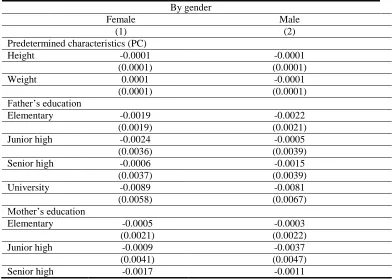
Table 4: Subsample regressions by gender (dependent variable: ARA) By gender
Female Male
(1) (2)
Predetermined characteristics (PC)
Height -0.0001 -0.0001
(0.0001) (0.0001)
Weight 0.0001 -0.0001
(0.0001) (0.0001)
Father’s education
Elementary -0.0019 -0.0022
(0.0019) (0.0021)
Junior high -0.0024 -0.0005
(0.0036) (0.0039)
Senior high -0.0006 -0.0015
(0.0037) (0.0039)
University -0.0089 -0.0081
(0.0058) (0.0067)
Mother’s education
Elementary -0.0005 -0.0003
(0.0021) (0.0022)
Junior high -0.0009 -0.0037
(0.0041) (0.0047)
(0.0049) (0.0054)
University -0.0213* -0.0109
(0.0093) (0.0110)
Temporary events (TE)
Disaster -0.0002 0.0003
(0.0005) (0.0002)
Log lost -0.0000 0.0002
(0.0004) (0.0004)
Log assistance -0.0002 -0.0002
(0.0005) (0.0006)
Constant 0.1945*** 0.1976***
(0.0170) (0.0167)
F-test 21.28 18.92
R2 0.04 0.05
N 14516 13201
Notes: The regressions include all variables within PC, TE, and X. Variables in X are not displayed for reading convenience. Robust standard error is in parentheses. *** Statistically significant at 1% level, ** at 5% level, * at 10% level.
Except those in column (6), the F-statistics in all specifications are statistically significant, which means that, together, all the estimated coefficients are not equal to zero. I found that there is a significant correlation between height, weight, and father’s education on risk aversion (Table-4 column (2) and (5)), and the direction is negative as expected. But, when I tried to control for other control variables X, the significance of these predetermined characteristics diminished (column (1)). We can also see that there is no significant correlation on temporary events variables (the number of disaster experienced, amount lost, and amount of assistance received) on ARA in all specifications.Next, the estimated coefficients for assets and being male are negative and significant. It should be noted, however, that there is a possibility of reverse causality in assets, in which a person who loves to take risk tends to make more money. Past assets have no significant correlation with ARA. The coefficient for education is somewhat mixed: a person with elementary education tend to be risk averse, but if that person is educated at the university or equivalent then that person tend to be risk loving. There is no observed correlation between ARA and the dependency ratio.Another variable within X that is significant is time preference, but again the result is mixed. It seems that if an individual’s time preference is up until category 4 (impatient) he/she tends to be risk loving, but for an individual with category 5 (very impatient) he/she becomes risk averse. This situation is consistent across all specifications.The coefficients for age and age-square are significant and has a U-shaped relationship with ARA, which suggests that people tend to love risk up until they reach the age of 26 (the turning point), which then they become risk averse. This is probably because people at age above 26 are already working and risky behaviour is less desirable. People with age above 26 are also more likely of being married and having a family, which makes them less willing to take risk. It should be noted that the estimated coefficient for age-square is very small, which indicates that the degree of risk aversion does not differ much from that before the turning point.
Subsample regressions
significant relationship between mothers educated at university level on their daughter’s risk aversion. Nonetheless, there is still no observed impact of height on both men and women. The regression results also found that there are no anomalies regarding time preference for male (not displayed in the table), in which being impatient is associated with being risk-loving. This finding shows that female’s behaviour is the significant contributor for the mixed result on time preference in Table 2.
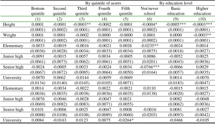
The estimations include subdistrict fixed effects and the standard errors are clustered at subdistrict level. The first part of Table-5 shows that disaster and the amount of assistance received (that related with the disaster) are, respectively, positively and negatively associated with risk aversion for individuals with assets at the second quintile (relatively poor in terms of assets value). This direction of these relationships is as expected. On the other hand, height is positively correlated with being risk-loving for individuals with assets at the third quintile (near poor). There is no consistent impact of parent’s education on individual’s risk aversion. With regard to time preference, I found that the anomalies (very impatient tend to be risk averse) occurred to people in the fourth and fifth assets quintiles (middle income and rich). Still, I cannot find a consistent relationship between PC and TE on ARA.
The second part of Table 5 is for regression by education level. A person is categorised as having ―Basic education‖ if that person is educated at elementary or junior high level as mandated by the Government Regulation 47/2008, and ―Higher education‖ if educated at senior high school and above. I found many anomalies here especially with regard to those who never/not been in school, that might be attributed to the respondent’s lack of understanding about the questions on risk aversion. Interestingly, height is significantly correlated with being risk-loving in all specifications, but this result might be caused by the omission of education from the regressions. This means that there is a positive correlation between education level and height.It would be more interesting to see how the interaction between various levels of assets and education can have different impact on risk preference. One can logically infer that education and endowment level should move in the same direction and the findings in Table 5 should also hold.
Table 5: Regressions by quintiles of assets and by education level (dependent variable: ARA) By quintile of assets By education level Bottom quintile Second quintile Third quintile Fourth quintile Fifth quintile Not/never school Basic education Higher education
(1) (2) (3) (4) (5) (6) (9) (10)
Height 0.0001 -0.0001 -0.0003** -0.0002 -0.0001 -0.0004* -0.0005*** -0.0003*** (0.0001) (0.0002) (0.0001) (0.0001) (0.0001) (0.0002) (0.0001) (0.0001) Weight 0.0001 0.0001 -0.0002 0.0000 -0.0000 0.0001 0.0000 -0.0003**
(0.0001) (0.0002) (0.0001) (0.0001) (0.0001) (0.0002) (0.0001) (0.0001) Elementary -0.0033 -0.0019 -0.0016 -0.0021 0.0026 -0.0235** -0.0024 0.0014
(0.0036) (0.0028) (0.0034) (0.0033) (0.0034) (0.0075) (0.0018) (0.0027) Junior high -0.0091 -0.0015 0.0057 0.0034 -0.0005 0.0086 -0.0052 0.0025
(0.0061) (0.0073) (0.0062) (0.0061) (0.0051) (0.0201) (0.0043) (0.0036) Senior high -0.0024 -0.0005 0.0033 -0.0024 0.0034 -0.0766*** -0.0066 0.0029
(0.0067) (0.0072) (0.0085) (0.0064) (0.0050) (0.0164) (0.0057) (0.0035) University -0.0070 0.0062 -0.0144 -0.0059 -0.0069 0.0014 -0.0070 (0.0134) (0.0140) (0.0165) (0.0105) (0.0071) (0.0183) (0.0047) Elementary 0.0014 -0.0034 -0.0022 0.0022 -0.0021 0.0110 -0.0015 0.0015
Notes: The regressions include all variables within PC, TE, and X except assets (column (1) to (5)) and education (column (6) to (8)). Variables in X are not displayed for reading convenience. Robust standard error is in parentheses. *** Statistically significant at 1% level, ** at 5% level, * at 10% level. The estimations include subdistrict fixed effects and the standard errors are clustered at subdistrict level.
But when we rearrange the variables and made another four subsamples based on the combination of education (those educated at higher level) and assets level (those within the fifth quintile assets), there is still no significant impact of variables in PC and TE on ARA10. One might suspect also that there is a reverse causality between ARA and time preference and married. There is another possibility as well that assets, lag of assets, rural, and impatience are influenced by the shock variables. I ran another regression that excludes those variables and found that while the estimated coefficients for height became significant, but the role of temporary events remains insignificant. Overall, the regressions in Table 3, 4 and 5 show the greater importance of demographic characteristics over predetermined characteristics or temporary events in explaining the variations in ARA. Still, there are limitations in these such as the sensitivity over different methods of measuring risk aversion, different ways to incorporate physical characteristics, possible impact of past economic shock, and the impact of abilities. Section 3.2 below will take a closer look over these potential problems.
Robustness check
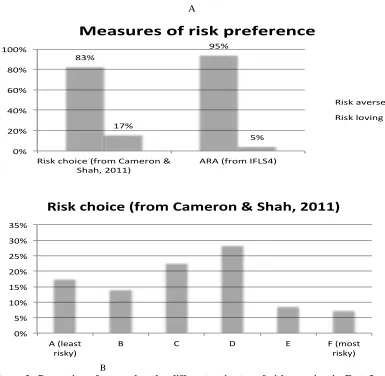
Before checking for the sensitivity from using different measure of risk aversion, it is interesting to see how different construction of risk aversion from different source can be resulted in a significantly different outcome. For example, Cameron and Shah (2011) were surveying individuals in East Java and come up with their own estimate of risk attitude. Comparing their estimate with the author’s estimate from the IFLS4 shows significant differences as shown in panel B and C in Figure 2.
10
The resultsarenot displayedheredue to the large size of the table. The output tables, however, are available upon request.
(0.0186) (0.0221) (0.0162) (0.0182) (0.0130) (0.0748) (0.0073) Disaster -0.0008 0.0011* 0.0001 0.0000 0.0020 -0.0068*** 0.0001 0.0003
(0.0006) (0.0006) (0.0005) (0.0001) (0.0043) (0.0010) (0.0003) (0.0003) Log lost 0.0004 0.0001 -0.0004 0.0004 0.0005 0.0028* -0.0002 0.0003
(0.0008) (0.0008) (0.0008) (0.0008) (0.0006) (0.0013) (0.0005) (0.0005) Log Assist. -0.0003 -0.0024* 0.0010 -0.0007 -0.0001 0.0025 -0.0008 0.0003
(0.0011) (0.0012) (0.0011) (0.0014) (0.0010) (0.0014) (0.0006) (0.0007)
F 10.63 10.88 10.38 8.46 18.59 . 13.95 17.01
R2 0.05 0.05 0.06 0.06 0.08 0.05 0.04 0.04
A
B
Figure 2: Proportion of respondent by different estimates of risk aversion in East Java, Indonesia
Source: Cameron and Shah (2011), author’s estimate
However, Cameron and Shah did not use the above categorical variable in their main estimation and re-categorise it into two categories: risk averse (if choose A-D) and risk loving (if choose E and F). If we also do such categorisation by giving a ―risk loving‖ label to those with ARA = 0.008 and ARA = 0.005, then the observed difference decrease quite substantially (panel A in Figure-2). It should be noted that the estimates are not directly comparable due to different survey period (Cameron and Shah’s survey was in 2008 while the IFLS4 was in 2007) and due to different estimation design. Cameron and Shah used real money in their experiment and the subjects were, interestingly, more willing to take risk compared to those in the IFLS4 where the subjects were not offered real money. Nonetheless, this study used data not only from one province (such as East Java) but also from all other provinces covered by the IFLS. The following paragraphs will observe how different estimation design may affect the outcome differently. First, we need to check for the sensitivity on the choice of the dependent variable by running full regressions as in equation (2), but using RL1 and RL2 instead of ARA as the dependent variable. The results are summarised in Table-6.Table-6 shows that almost all predetermined characteristics and temporary events are not significant, supporting the results from the main regressions. Nonetheless, father’s education at the university
83%
95%
17%
5%
0% 20% 40% 60% 80% 100%
Risk choice (from Cameron & Shah, 2011)
ARA (from IFLS4)
Measures of risk preference
Risk averse
Risk loving
0% 5% 10% 15% 20% 25% 30% 35%
A (least risky)
B C D E F (most
and mother’s education at junior high school are significant in some of the regressions. Other variables such as age, age-square, higher degree education, and being very impatient remain significant and exhibiting the same direction as in the main regressions. In addition to that, except for being very impatient, other category of impatience loses its significance. Surprisingly, the constants seem to be not significant in all of these OLS specifications.The author also redid subsample regressions based on assets and education and the results are fairly similar. While RL2 provides support for a positive relationship between height and risk loving behaviour for people on the third quintile, but in general the evidence that PC and TE can explain variations in risk aversion is limited.
Table 6: Sensitivity in the dependent variable
OLS
Dependent variable RA RL1 RL2
(1) (2) (3)
Height 0.0002 0.0000 -0.0001
(0.0006) (0.0002) (0.0001)
Weight 0.0011 0.0002 0.0003*
(0.0007) (0.0002) (0.0001)
Elementary 0.0105 0.0052 -0.0041
(0.0168) (0.0058) (0.0037)
Junior high -0.0248 -0.0065 -0.0063
(0.0310) (0.0101) (0.0065)
Senior high -0.0101 -0.0051 -0.0054
(0.0343) (0.0116) (0.0079)
University 0.1683* 0.0326 0.0299
(0.0681) (0.0235) (0.0160)
Elementary 0.0234 0.0099 0.0069
(0.0186) (0.0063) (0.0037)
Junior high 0.0938* 0.0258* 0.0114
(0.0366) (0.0118) (0.0083)
Senior high 0.0515 0.0228 -0.0029
(0.0492) (0.0164) (0.0111)
University 0.1485 0.0180 0.0122
(0.0999) (0.0314) (0.0256)
Disaster 0.0024 0.0016 0.0016
(0.0086) (0.0028) (0.0024)
Lost (ln) -0.0019 -0.0010 -0.0004
(0.0041) (0.0013) (0.0009)
Assistance (ln) 0.0028 0.0004 0.0001
(0.0056) (0.0018) (0.0013)
Assets (ln) 0.0155** 0.0033* 0.0022*
(0.0047) (0.0016) (0.0010)
Lagged assets (ln) 0.0027 0.0018 -0.0001
(0.0033) (0.0011) (0.0008)
Muslim 0.0046 0.0011 0.0034
(0.0403) (0.0125) (0.0079)
Javanese -0.0104 -0.0028 -0.0045
(0.0259) (0.0080) (0.0061)
Rural 0.0095 0.0030 -0.0064
(0.0370) (0.0125) (0.0076)
OLS
Dependent variable RA RL1 RL2
(1) (2) (3)
(0.0023) (0.0008) (0.0005)
Age^2 -0.0001*** -0.0001*** -0.0000*
(0.0000) (0.0000) (0.0000)
Sex 0.2411*** 0.0669*** 0.0294***
(0.0161) (0.0058) (0.0033)
Married -0.0115 0.0003 0.0011
(0.0171) (0.0062) (0.0034)
Dependency -0.0028 0.0073 -0.0107
(0.0348) (0.0121) (0.0069)
Patient 0.0681 0.0031 0.0156
(0.0533) (0.0198) (0.0127)
Somewhat impatient -0.0369 -0.0574** -0.0078
(0.0557) (0.0206) (0.0123)
Impatient -0.0149 -0.0367 -0.0157
(0.0548) (0.0197) (0.0121)
Very impatient -0.2283*** -0.0586** -0.0163
(0.0501) (0.0181) (0.0114)
Elementary -0.0377 0.0003 -0.0119*
(0.0273) (0.0104) (0.0056)
Junior high -0.0289 -0.0084 -0.0000
(0.0311) (0.0122) (0.0066)
Senior high 0.0040 0.0003 0.0028
(0.0333) (0.0131) (0.0072)
University 0.1680*** 0.0396* 0.0273**
(0.0423) (0.0154) (0.0096)
Constant 0.1399 -0.0151 -0.0050
(0.1445) (0.0510) (0.0293)
F 21.852 10.137 7.668
2
R2 0.04 0.02 0.01
N 27717 27717 27717
Notes: robust standard error is in parentheses. *** statistically significant at 1% level, ** at 5% level, * at 10% level. OLS estimations include subdistrict fixed effects and the standard errors are clustered at subdistrict level.
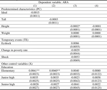
Another robustness check is by using a dummy variable Ideal as a proxy for physical prowess that is derived from the body mass index (BMI). BMI is simply the ratio between the weight (kg) and the square of height (meter). The variable Ideal equals to 1 if the BMI is at normal range (between 18.5 to 25 as defined by the WHO)11. Another alternative measure is relative height, which is a dummy variable Tall, which equals to 1 if the person is taller than the median of other respondents of the same sex living in the same district12. As can be seen in column (1) and (2) of Table-7, the use of either Ideal or Tall as an alternative measure of physical attribute cannot help explaining variations in ARA. While economic shock is relevant for Indonesia (the country experienced the 1997/1998 Asian economic crisis) and there are studies that shows the impact of the crisis on different households or economic sectors (Fallon and Lucas, 2002, Waters et al. 2003, Wie, 2000), but the information on individual risk preference is only available in 2007. There are also various
11
See http://apps.who.int/bmi/index.jsp?introPage=intro_3.html
12
factors affecting the individual within that 10-year gap that might not be observed. It is also difficult to identify the impact of the crisis for different individuals or to know if an individual’s observed behaviour is due to the crisis.Nonetheless, I tried to control for the crisis by adding three variables: Ecshock, change in the poverty rate, and the interaction between these two. Ecshock is a dummy variable that equals to 1 if the respondent worked in the construction and financial sector in 1997 by utilising data from IFLS2. These two economic sectors got the hardest hit (based on the drop in real GDP growth) during the crisis (Wie, 2000). In Table-7 column (3) we can see that there is no observed impact of past crisis on current risk preference. It should be noted that since the number of respondent increased between IFLS2 and IFLS4 and not all respondent worked during the IFLS2 survey, the final number of observation is severely limited.
Again, subsample regressions cannot explain variations in ARA when I varied the measure for physical attributes (Tall and Ideal) or when I control for the impact of past shock.Finally, I controlled for cognitive ability and numerical ability in Table-7 column (4) because I also used education as one of the explanatory variables in X. Excluding ability will bias the estimated coefficient of education. However, question on ability is limited only to respondent age 15-24, which reduces the number of observation. The estimation shows that education variable became insignificant and numerical ability is strongly and negatively correlated with ARA, indicating that people with high mathematical ability tend to be more risk loving. This result is confirmed when I used subsample regressions where the numerical ability is significant and negatively associated with risk averseness for people in the third and fifth endowment quintiles. This is somewhat an important result because we observe that the coefficients for elementary and higher degree education are statistically significant throughout all specification in the main regression (Table-4).
Table 7: Ideal posture, economic crisis, and abilities Dependent variable: ARA
(1) (2) (3) (4)
Predetermined characteristics (PC)
Ideal -0.0015
(0.0011)
Tall -0.0003
(0.0011)
Height -0.0002* -0.0001
(0.0001) (0.0001)
Weight 0.0000 0.0000
(0.0001) (0.0001)
Temporary events (TE)
Ecshock 0.0086
(0.0055)
Change in poverty rate -0.0029
(0.0044)
Shock -0.0053
(0.0069) Other control variables (X)
Education
Elementary 0.0061** 0.0060** 0.0040 0.0080
(0.0023) (0.0023) (0.0032) (0.0122)
Junior high 0.0035 0.0035 -0.0023 0.0058
(0.0025) (0.0025) (0.0042) (0.0123)
Senior high -0.0028 -0.0027 -0.0041 0.0022
Dependent variable: ARA
(1) (2) (3) (4)
University -0.0145*** -0.0145*** -0.0112* -0.0074
(0.0033) (0.0033) (0.0052) (0.0128)
Cognitive ability 0.0014
(0.0049)
Numerical ability -0.0161***
(0.0035)
Constant 0.1887*** 0.1875*** 0.2381*** 0.1936***
(0.0092) (0.0091) (0.0234) (0.0296)
F 44.82 44.79 14.46 15.78
R2 0.06 0.06 0.06 0.05
N 27717 27717 8965 10642
Notes: The regressions also include all variables within PC, TE, and X. Variables in X are not displayed for reading convenience. Robust standard error is in parentheses. *** statistically significant at 1% level, ** at 5% level, * at 10% level. The estimations include subdistrict fixed effects and the standard errors are clustered at subdistrict level.
Insurance policy
Cameron and Shah, (2011) observed that people who lived in disaster-prone area in East Java tend to self-insure through a rotating saving mechanism (Arisan) and they also found that receiving remittance offset some of the impact of natural disaster on risk aversion. In order to test this I included a dummy for the participation in Arisan and the amount of transfer received from outside the household (Transfer, in natural logarithm). Table-8 shows that people who experience disaster are, on average, have higher transfer and involve more in Arisan.
Table 8: Self-insurance and natural disaster
Disaster No disaster Difference
Arisan 0.3865
(0.0113)
0.2230
(0.0026) 0.1635***
Transfer (ln) 8.6102
(0.2116)
7.7545
(0.0566) 0.8557***
N 1868 25849
Note: *** significant at 1% level
I then interacted these variables with how often the individual experienced disaster (Arisan × Disaster and Transfer × Disaster) and included these in the full regression (equation (2)). If the estimated coefficient for Transfer × Disaster is negative and significant, it means that the larger the transfer, the less risk averse the individual when there is a shock (disaster). Hence, these additional variables can be seen as an informal proxy for the demand for a disaster-related insurance.
Table 9: Self-insurance (dependent variable: ARA)
Full sample Subsample
Not Arisan Arisan
(1) (2) (3)
Arisan -0.0030*
(0.0014)
Arisan × disaster 0.0008*
(0.0003)
Transfer (ln) -0.0002** -0.0002* -0.0002
Transfer × disaster -0.0001 -0.0001 -0.0002
(0.0001) (0.0001) (0.0001)
Constant 0.2046*** 0.2074*** 0.1825***
(0.0117) (0.0117) (0.0117)
F-test 38.78 32.53 12.22
R2 0.06 0.06 0.07
N 27707 21220 6487
Notes: The regressions also include all variables within PC, TE, and X. Variables in PC, TE, and X are not displayed for reading convenience. Robust standard error is in parentheses. *** statistically significant at 1% level, ** at 5% level, * at 10% level. The estimations include subdistrict fixed effect and the standard error is clustered at subdistrict level.
In Table 9 column (1), I found that while Arisan is negatively correlated with ARA but the coefficient for Arisan × Disaster is positive and significant. This means that after controlling for the direct impact of the Arisan, an individual tend to be more risk averse when he/she experienced (more) disaster. On the other hand, only the coefficient for Transfer is negative and significant, which suggests that only the direct effect of Transfer that drives risk aversion. Overall, these results give less support for a natural disaster-related insurance policy.Nonetheless, we might suspect that Arisan has reverse causality with ARA: risk-averse individuals tend to involve more in such rotating saving mechanism to smooth their consumption. Therefore, I made subsample regressions by Arisan participation in column (2) and (3). The estimated coefficients do not differ much from those in column (1), thus support the previous claim that only Transfer that determines ARA.
CONCLUDING REMARKS
Several studies point out to the important role of temporary shocks and predetermined characteristics on determining an individual’s risk preference. My observation using IFLS4 data for Indonesia shows that this is not necessarily the case: only father’s education at higher level that exhibits the expected sign and significance. The impact of natural disaster as found in Cameron and Shah (2011) diminished when I use full sample of both the rural and urban area. Physical attributes were showing significance and correlates negatively with ARA in regressions that contain predetermined characteristics and shock variables, but then fell down when I control for demographic variations and other variables. Nonetheless, there is a strong correlation as well between being impatient with low degree of ARA (risk-loving). These give preliminary indication that variations in risk preference are indeed random.
research in this topic is by Tanaka et al. (2010) where they found that poor villagers in Vietnam are not always fear of uncertainty in income variation, but they also fear of loss. This will be the future direction of this study.
Appendix
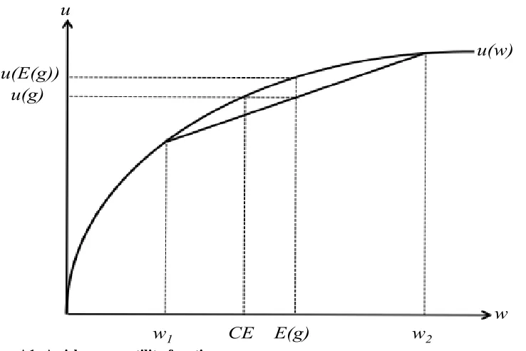
Risk-averse individual
Consider an individual that has a von Neumann-Morgenstern (VNM) utility function over wealthu w . Consider also that there is a simple gamble g that has an expected value ofE g =
piwi, where pi is the probability of winning wealth wi. Suppose that the person is asked to
choose to either: (1) engaged in a gamble g, or (2) getting an amount E g with certainty. A risk-neutral individual will have a linear utility function and sees these two options indifferently because the expected value from engaging in the gamble is simply equal toE g . However, for a person who is not risk-neutral, he/she should consider the utility for each possible wealth resulted from the gamble. Therefore, he/she compared u g = piu wi of Option (1) and u E g =
u piwi of Option (2).
Figure A1: A risk averse utility function
A risk-averse individual is someone who choose (2) over (1), that is if u E g > 𝑢 g , as shown in Figure A1 above. This is because a risk-averse individual will choose a certain amount of wealth
CE that generates the same level of utility as u g , even though the gamble’s expected value
E g > 𝐶𝐸.
E(g)
CE
w
1w
2u(E(g))
u(g)
u(w)
Table A1:Questions on risk preference in IFLS4
Table A2: Constructing time preference
Respondent’s choice Forgone amount Time
preference Definition
Rp1 million in 1 year Rp1 million today 1 Very patient
Rp2 million in 1 year Rp1 million today 2 Patient
Rp1 million today Rp2 million in 1 year 3 Somewhatimpatient
Rp6 million in 1 year Rp1 million today 4 Impatient
Rp1 million today Rp6 million in 1 year 5 Very impatient
Table A3: Questions on time preference in IFLS4
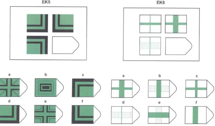
Measuring ability
Both cognitive ability (ca) and numerical ability (na) is measured by assigning a value of 1 (and 0 otherwise) if the person chooses the correct answer from questions on logic in IFLS4 (section EK). There are 8 questions on cognitive ability in which the respondent (age 15-24) was asked to choose a shape that match with the 3 existing shapes in each question (see Figure A2 below). There are only 5 questions on numerical ability (Table-A4) that asked standard mathematical problems of elementary-junior high school level.
Table A4: Numerical ability
REFERENCES
Ball, S. (2010). Risk aversion and physical prowess: Prediction, choice and bias. Journal of Risk and Uncertainty, Vol. 41, pp. 167-193.
http://www.springerlink.com/content/n1r0760l43180703/ Accessed on 17 September (2012).
Bisnwanger, H. P. (1980). Attitudes toward Risk: Experimental Measurement in Rural India.
American Journal of Agricultural Economics, August (1980).
BONIN, H. (2007). Cross-sectional earnings risk and occupational sorting: The role of risk attitudes. Labour Economics, Vol. 14, pp. 926-937.
http://www.sciencedirect.com/science/article/pii/S0927537107000462 Accessed on 9
August (2012).
CAMERON, L. & SHAH, M. (2011). Risk-Taking Behavior in the Wake of Natural Disasters. Discussion paper, working paper, University of California- Irvine,
http://users.monash.edu.au/~clisa/papers/NatDisJuly6_2011.pdf Accessed on 7 August
(2012).
CESARINI, D. (2009). Genetic Variation in Preferences for Giving and Risk Taking. The Quarterly Journal of Economics,Vol. 124, pp. 809-842, http://qje.oxfordjournals.org/
Accessed on 29 August ( 2012).
CIPOLLONE, A. (2011). Education as a Precautionary Asset.
http://ideas.repec.org/p/pra/mprapa/34575.html Accessed on 29 August (2012).
CRAMER, J. S. (2002). Low risk aversion encourages the choice for entrepreneurship: an empirical test of a truism. Journal of Economic Behavior & Organization, Vol. 48, pp.
29-36, http://ideas.repec.org/a/eee/jeborg/v48y2002i1p29-36.html Accessed on 8 August
(2012).
DANG, A. D. (2012). On the Sources of Risk Preferences in Rural Vietnam. ANU RSE Working Paper, July 2012, http://mpra.ub.uni-muenchen.de/38738/ Accessed on 7 August (2012). DOHMEN, T. (2008). The Intergenerational Transmission of Risk and Trust Attitudes. CESifo
DOHMEN, T. (2009). Individual Risk Attitudes: Measurement, Determinants and Behavioral Consequences. Research Memorandum, http://arno.unimaas.nl/show.cgi?fid=15550
Accessed on 7 August 2012.
DOW, J. & WERLANG, S. R. D. C. (1992). Uncertainty Aversion, Risk Aversion, and the Optimal Choice of Portfolio. Econometrica, Vol. 60, pp. 197-204.
http://www.jstor.org/stable/2951685?origin=JSTOR-pdf Accessed on 7 August (2012).
FALLON, P. R. & LUCAS, R. E. B. (2002). The Impact of Financial Crises on Labor Markets, Household Incomes, and Poverty: A Review of Evidence. World Bank Research Observer, Vol. 17, pp. 21-45.http://wbro.oxfordjournals.org/content/17/1/21.short Accessed on 20 September (2012).
GADUH, A. (2012). Religion, social interactions, and cooperative attitudes: Evidence from Indonesia. University of Southern California (Preliminary draft), March 2012,
http://papers.ssrn.com/sol3/papers.cfm?abstract_id=1991484 Accessed on 29 August (2012).
GUISO, L. & PAIELLA, M. (2005). The role of risk aversion in predicting individual behavior. Bank of Italy Working Paper Series, http://repec.org/esLATM04/up.5136.1082045630.pdf
Accessed on 7 August 2012.
GUISO, L. & PAIELLA, M. (2008). Risk Aversion, Wealth, and Background Risk. Journal of the European Economic Association,
http://ideas.repec.org/a/tpr/jeurec/v6y2008i6p1109-1150.html Accessed on 7 August (2012).
HOLT, C. A. & LAURY, S. K. (2002). Risk Aversion and Incentive Effects. The American Economic Review, Vol. 92, pp. 1644-1655.
http://www.jstor.org/stable/3083270?origin=JSTOR-pdf Accessed on 6 August (2012).
HRYSHKO, D. (2011). Childhood determinants of risk aversion: The long shadow of compulsory education. Quantitative Economics, Vol. 2, pp. 37-72.
http://onlinelibrary.wiley.com/doi/10.3982/QE2/abstract Accessed on 30 August (2012).
HÜBLER, O. (2012). Are Tall People Less Risk Averse Than Others? SOEP papers,
http://ssrn.com/abstract=2039567 Accessed on 8 August 2012.
HURST, E. & LUSARDI, A. (2004). Liquidity Constraints, Household Wealth and Entrepreneurship. Journal of Political Economy, 112
http://www.jstor.org/stable/10.1086/381478 Accessed on 18 October (2012).
KAHNEMAN, D. & TVERSKY, A. (1979). Prospect Theory: An Analysis of Decision under Risk.
Econometrica, Vol. 47, pp. 263-292, http://www.jstor.org/stable/1914185?origin=JSTOR-pdf Accessed on 5 February (2011).
KORNIOTIS, G. & KUMAR, A. (2012). Stature, Obesity, and Portfolio Choice.
http://papers.ssrn.com/sol3/papers.cfm?abstract_id=1509173 Accessed on 30 August (2012).
LE, A. T. (2011). Attitudes towards economic risk and the gender pay gap. Labour Economics, Vol. 18, pp. 555-561,
http://genepi.qimr.edu.au/contents/p/staff/Le_LabEconomics_555-561_2011.pdf Accessed on 9 August (2012).
MACHINA, M. J. (1987). Choice Under Uncertainty: Problems Solved and Unsolved. Journal of Economic Perspectives, Vol. 1, No. 1
MALMENDIER, U. & NAGEL, S. (2011). Depression Babies: Do Macroeconomic Experiences Affect Risk Taking. The Quarterly Journal of Economics, 126, 373–416,
http://qje.oxfordjournals.org/ Accessed on 6 August (2012).
PERMANI, R. (2011). Revisiting the Link between Maternal Employment and School-Aged Children Health Status in Developing Countries: An Instrumental Variable Approach. The University of Adelaide School of Economics, Research Paper No. 2011-21
http://www.economics.adelaide.edu.au/research/papers/doc/wp2011-21.pdf Accessed on 29
August 2012.
PRATT, J. W. (1964). Risk Aversion in the Small and in the Large. Econometrica, 32, 122-136,
http://www.jstor.org/stable/1913738 Accessed on 30 October 2012.
RUBIN, P. H. & PAUL, C. W. (1979). An Evolutionary Model of Taste for Risk. Economic Inquiry, Vol. 17, pp. 585-596,
SCHOEMAKER, P. J. H. (1993). Determinants of Risk-Taking: Behavioral and Economic Views.
Journal of Risk and Uncertainty, Vol. 6, pp. 49-73.
http://imap.whartonmackcenter.com/files/0/4/443/Schoemaker, Paul J.H. Determinants of
Risk-Taking-Behavioral and Economic Views.pdf Accessed on 30 October 2012.
STIGLER, G. J. & BECKER, G. S. (1977). De Gustibus Non Est Disputandum. American Economic Review, 67, 76-90, http://www.jstor.org/stable/1807222 Accessed on 17 September (2012).
TANAKA, T. (2010). Risk and Time Preferences: Linking Experimental and Household Survey Data from Vietnam. American Economic Review, Vol. 100, pp. 557-571.
http://www.aeaweb.org/articles.php?doi=10.1257/aer.100.1.557 Accessed on 23 September
(2012).
VAN DEN BERG, M. (2009). Natural Hazards And Risk Aversion: Experimental Evidence From Latin America. Paper prepared for the International Association of Agricultural Economists Conference, Beijing, China, 2009, http://ideas.repec.org/p/ags/iaae09/51394.html Accessed on 7 August (2012).
WATERS, H. (2003). The impact of the 1997–98 East Asian economic crisis on health and health care in Indonesia. Health Policy and Planning, Vol. 18, pp. 178-181.
http://heapol.oxfordjournals.org/content/18/2/172.short Accessed on 20 September (2012).
WIE, T. K. (2000). The Impact of the Economic Crisis on Indonesia's Manufacturing Sector. The Developing Economies, pp. 420-453.