Enhanced Color Correction Using Histogram Stretching Based On Modified Gray World and White Patch Algorithms

Enhanced Color Correction Using Histogram

Stretching Based On Modified Gray World and

White Patch Algorithms

Department Of Computer Science ,Guru Nanak Dev University, Amritsar.

Abstract—Color constancy is the capability to determine colors of objects independent of the color of the light source. This paper deals with the different color constancy algorithms to evaluate the performance of existing color constancy algorithms. The combined effect of two color constancy algorithms i.e. White Patch Retinex (WPR) and Gray World (GW) and gamma correction used for dynamic range correction for image enhancement. The main limitation of the color constancy integrated with gamma correction proves to be efficient for dark regions but produce poor results for brighter regions. To reduce this problem in this paper we have proposed a new algorithm which will integrate the color constancy with histogram stretching and average filter to provide accurate results in dark, medium and brighter regions. The proposed algorithm is designed and implemented in MATLAB using image processing toolbox. The proposed algorithm provides significant as it has shown significantly better results in poor, high and medium intensity images as well as it reduce noise which may be introduced during color correction time.

Index terms: Color constancy, Gamma correction, Histogram Stretching, Average Filter, illumination.

1. INTRODUCTION

Image processing is a technique to convert an image into digital form and perform some operations on it, in order to get an enhanced image or to extract some useful information from it. It is a type of signal dispensation in which input is image, like video frame or photograph and output may be image or characteristics associated with that image.

Color [1-12] is an significant cue for computer vision and image processing related topics, like feature extraction, human computer interaction, and color appearance models. Color vision is a process by which organisms and machines are able to distinguish objects based on the different wavelengths of light reflected, transmitted, or emitted by that object. Colors observed in images are determined by the fundamental assets of objects and surfaces, as well as the color of the illuminant. For a robust color-based system, the effects of the illumination should be filtered out. Color Constancy is the ability to identify the correct colors, independently of the illuminant present in the scene. Human vision has a natural capability to correct the color effects of the light source. On the other hand, the mechanism that is involved in this capability is not yet fully understood. The same process is not trivial to machine vision systems in an unconstrained scene.

1.1. Color Constancy:

Color constancy[1] is a mechanism of detection of color independent of light source. It is a characteristic of the individual color perception system which ensures that the perceived color of objects remains relatively constant under altering illumination conditions.

Figure.1.1 Illustration of the influence of differently colored light sources on the measured image values.

The color of objects is primarily effected [11] by the color of the light source. The analogous object, taken by the same camera but under different light, may vary in its measured color appearance. This color variation may negatively affect the result of image and video processing methods for different applications such as image segmentation, object recognition and video retrieval. The principle of color constancy is to eliminate the effect of the color of the light source. a significant number of color constancy algorithms has been proposed. color constancy is intrinsically an ill-posed problem, different assumptions have been proill-posed, such as the White-Patch assumption and the Grey-World assumption. Consider the images in Fig. 1. These images show the same scene, provided under four different light sources.

1.2 Gamma Correction:

To explain the gamma correction we consider computer monitor example, whose intensity to voltage response curve which is roughly a 2.5 power function, it means range of voltages sent to the monitor is between 0 and 1, then it will actually display a pixel which has intensity equal to x ^ 2.5. This means that the intensity value displayed will be less than what you wanted it to be. (e.g. 0.5 ^ 2.5 = 0.177) here, are said to have gamma of 2.5 .

Figure 1.2.Here, output from monitor f = v^2.5 _{, where f is}

pixel intensity and v is voltage.

The task of gamma correction is accomplished by raising the input value to the 1/2.5 power.

Figure 1.3.Here, gamma corrected output f = v^(1/2.5)

The luminance nonlinearity introduced by many imaging devices is described with an operation of the form

g f (x, y) = f (x, y) Eq(5)

where fi(x, y) ∈ [0, 1] denotes the image pixel intensity in

the component i. If the value of γ is known, then the inverse process is trivial

g f (x, y) = f (x, y) Eq(6)

The value of γ is determined experimentally with the aid of a calibration target taking a full range of known luminance values through the imaging system.

1.3 Color Constancy Algorithms:

We discuss about the two basics algorithms[1] of color constancy i. e. White Patch Retinex (WPR) and Gray World (GW).

1.3.1 White Patch Retinex:

White Patch Retinex[15] Algorithm is based on retinex theory by Edwin H. Land in 1971.This algorithm[8]

assumes that the highest value of each color channel as white representation of image. White patch found searching for the maximum intensity in each channel, is given by

I = max f (x, y) Eq(1)

where fi(x, y) is pixel intensity at position (x,y) in an image

and Ii is the illuminant in the scene.

All pixel intensities are scaled according to the illuminant computed:

o (x, y) =f (x, y)

I Eq(2)

1.3.2 Gray World:

The Gray World assumption[8] is a white balance method that assumes that your scene is neutral gray. It produce an estimate of illuminant by computing the mean of each channel of the image.

This algorithm suggests that the average value of R, G and B components to the common gray value. To normalize the image channel i, the pixel value is scaled by

Si = Eq(3)

where avgi is the channel mean and avg is the illumination

estimate.

Another method of normalization is normalizing to the maximum channel by scaling by si

r =max(avg , avg , avg )

avg Eq(4)

1.4 Average Filter:

An moving average filter[14] is utilized to reduce the noises. Mean filtering is a simple, intuitive and easy to implement method of smoothing images, i.e. reducing the amount of intensity variation between one pixel and the next. It is often used to reduce noise in images.

The scheme of mean filtering is simply to replace each pixel value in an image with the mean value of its neighbors, including itself. Generally, a 3×3 square kernel is used.

As shown in Figure 1, although larger kernels (e.g. 5×5 squares) can be used for more severe smoothing.

In above Figure.1.4 used the 3*3 moving average filter.

Each pixel has been replaced by the average of pixel values in a 3*3 square .The result is to reduce noise in the image.

1.5 Histogram Stretching:

Histogram stretching[13] balances the range of pixel intensity values and distribute over the entire histogram. Histogram stretching intends to distribute the

pixel exterior frequencies over the entire width of the histogram. It can modify the histogram in such a way to distribute the intensities on the scale of values available as well as possible and extend the histogram so that the value of the lowest intensity is zero and that of the highest is the maximum value. The stretching provides a better distribution in order to make light pixels even lighter and dark pixels closer to black.

Color histograms are three separate histograms i.e. R, G and B channels and are representation of distribution of each color in an RGB image. For a digital image, the color histogram is simply acquired rich source of information, the majority of the high-end cameras use color histogram as a reference of exposure and white balance set to see whether an unique color channel clips. A peak in the red, green and blue histograms when we shoot a scene, if the peaks in all the three channels are in the same place, then the image is impartial and the color temperature is set correctly. If not, then it is necessary to change the color temperature set of the camera. For example, if the blue channel is greatly towards highlights, then the scene is too greatly bluish and we should adjust the color temperature or white balance consequently.

Figure.1.5. Histogram Stretching Example.(adapted from [13])

2. PERFORMANCE METRICS

The quality of an image is examined by objective assessment as well as subjective assessment. For subjective assessment, the image has to be observed by a human expert. The human visual system is so intricate that it is not yet modeled correctly. As a result, besides objective assessment, the image must be observed by a human expert to judge its quality. There are various metrics[17] used for objective assessment of an image. Some of them are mean squared error (MSE), mean absolute error (MAE) and peak signal to noise ratio (PSNR).

2.1 Mean Squared Error (MSE):

Mean square error is a measure of image quality index. The large value of mean square means that image is a poor quality. Mean square error between the reference image and the fused image is

MSE = 1

mn (A − B ) Eq(5)

Where Ai, j and Bi, j are the image pixel value of reference image.

2.2. Root Mean Square Error:

It is the square root of the MSE.

RMSE = √MSE Eq(6)

2.3.Normalized Absolute Error (AE):

The large value of normalized absolute error means that image is poor quality. NAE is defined as follows

NAE =∑ _∑∑ ( A − B )_{∑ (A )} Eq(7)

2.4 Peak Signal to Noise Ratio (PSNR):

PSNR computes the peak signal-to-noise ratio, in decibels, between two images. This ratio is used as a quality measurement between the original and a reconstructed image. The higher the PSNR, the better is the quality of the reconstructed image. To compute the PSNR, first we have to compute the mean squared error (MSE) using the following equation.

MSE = 1

mn (A − B ) Eq(8)

PSNR = 10 ∗ log (peak

MSE) Eq(9)

PSNR value should be as high as possible.

2.5 Normalized Cross Correlation (NCC):

Normalized cross correlation is used to find out similarities between fused image and registered image is given by the following equation:

NCC = A ∗ B Eq(10)

3. EXPERIMENTAL SET-UP

In order to implement the proposed algorithm, design and implementation has been done in MATLAB using image processing toolbox. In order to do cross validation we have implemented the edge based color constancy with bilateral filter. Table 1 is showing the various images which are used in this research work. Images are given along with their formats. All the images has different kind of the light i.e. more or less in some images.

Table 1. Experimental Images

S.No NAME FORMAT

1 image1 TIF

2 image2 JPEG

3 image3 JPEG

4 image4 JPEG

5 image5 JPEG

6 image6 JPEG

7 image7 JPEG

8 image8 JPEG

9 image9 JPEG

3.1 Experimental results:

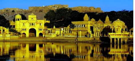
Figure 3.1 has shown a temple image which is infected by sun light. It has been clearly shown that the image demands constancy.

Figure 3.1 Input images

Figure 3.2 has shown the result of Gamma corrected image. It has been clearly shown the effect of the light has been removed.

Figure 3.2 Gamma corrected image

Figure 3.3 has demonstrated the result of White Patch algorithm. It has shown the better results than the result of the gamma correction.

Figure 3.3 White Patch Image

3.4 has shown the result of Gamma Correction with White Patch Image based color constancy. It has been clearly shown the effect of the light has been removed at a great extent than images shown in figures 3.2 and 3.3.

Figure 3.4 Gamma Correction With White Patch Image

3.5 has shown the result of White Patch with Gamma Correction Image based color constancy. It has been clearly shown the effect of the light has been removed very efficiently than images shown in figures 3.2,3.3 and 3.4.

Figure 3.5 White Patch With Gamma Correction

Figure 3.6 has shown the result of the proposed algorithm. It has been clearly demonstrated that the proposed algorithm has better visibility than the images given in figures 3.1, 3.2, 3.3, 3.4 and 3.5. Thus proposed algorithm provides better results.

Figure 3.6 Final Filtered Image with White Patch

Figure 3.7 has demonstrated the result of Gray world algorithm. It has shown the better results than the result of the gamma correction.

Figure 3.7 Gray World Image

Figure 3.8 Gamma Correction with Gray World Image

Figure 3.9 has clearly shown the effect of the light has been removed very efficiently than images shown in figures 3.2,3.7 and 3.8

3.9 Gray World with Gamma Correction Image

Figure 3.10 has shown that the proposed algorithm has better visibility than the images given in figures 3.1, 3.2,3.7,3.8 and 3.9.

3.10 Final Filtered Image with Gray World

4. PERFORMANCE EVALUATION

This section contains the cross validation between existing and proposed techniques. Some well-known image performance parameters for digital images have been selected to prove that the performance of the proposed algorithm is quite better than the available methods.

4.1 Performance Evaluation With White Patch Algorithm:

Table 2 has shown the quantized analysis of the Mean Square Error. As mean square error need to be reduced therefore the proposed algorithm is showing the better results than the available methods as mean square error is less in every case.

Table 2. Mean Square Error

Image Name

Gamma Correction

White Patch

Gamma Correction

with White Patch

White Patch with Gamma Correction

Proposed

Img1 607 454 114 117 3

Img2 868 773 185 190 135

Img3 661 19 242 232 1

Img4 372 271 104 102 1

Img5 446 10 306 294 13

Img6 346 89 200 188 3

Img7 314 87 87 81 17

Img8 552 18 327 310 1

Img9 758 2 360 343 17

Img10 856 1 247 237 3

Table 3 is showing the comparative analysis of the Root Mean Square Error. It has clearly demonstrated that the root mean square error is quite less in the case of the proposed algorithm; therefore proposed algorithm is providing better results.

Table 3. Root Mean Square Error

Image Name

Gamma Correction

White Patch

Gamma Correction

with White

Patch

White Patch with Gamma Correction

Proposed

Img1 51.0588 21.3073 10.6771 10.8167 1.7321

Img2 96.2705 27.8029 13.6015 13.7840 11.6190

Img3 79.7559 4.3589 15.5563 15.2315 1

Img4 127.5617 16.4621 10.1980 10.0995 1

Img5 127.0669 3.1623 17.4929 17.1464 3.6056 Img6 96.6747 9.4340 14.1421 13.7113 1.7321

Img7 130.4377 9.3274 9.3274 9 4.1231

Img8 120.6317 4.2426 18.0831 17.6068 1

Img9 150.8575 1.4142 18.9737 18.5203 4.1231

Img10 88.6341 1 15.7162 15.3948 1.7321

Table 4 is showing the comparative analysis of the Normalized Absolute Error. It contains the average difference between input and output image. Table 4 has clearly demonstrated that the Mean Absolute Error is quite less in the case of the proposed algorithm; therefore proposed algorithm is providing better results.

Table 4. Normalized Absolute Error

Image Name

Gamma Correction

White Patch

Gamma Correction

with White Patch

White Patch with Gamma Correction

Proposed

Img1 0.5715 0.4034 0.1772 0.1778 0.0351

Table 5 is showing the comparative analysis of the Peak Signal to Noise Ratio (PSNR). As PSNR need to be maximized; so the main goal is to increase the PSNR as much as possible. Table 5 has clearly shown that the PSNR is maximum in the case of the proposed algorithm therefore proposed algorithm is providing better results than the available methods.

Table 5. Peak Signal to Noise Ratio

Image Name Gamma Correction White Patch Gamma Correction with White Patch White Patch with Gamma Correction Proposed

Img1 13.9694 21.5597 27.5520 27.4368 42.4822

Img2 8.4605 19.2437 25.4396 25.3295 26.8192

Img3 10.0954 35.1505 24.2841 24.4663 47.4439

Img4 6.0164 23.7921 27.9534 28.0433 47.3441

Img5 6.0500 38.1278 23.2619 23.4405 36.8116

Img6 8.4244 28.6345 25.0991 25.3862 42.6337

Img7 5.8227 28.7048 28.7136 29.0410 35.6071

Img8 6.5014 35.5759 22.9734 23.2116 45.7293

Img9 4.5594 43.6373 22.5629 22.7728 35.7962

Img10 9.1786 48.0111 24.1955 24.3723 43.2304

Table 6 shows the comparative analysis of the Normalized Cross-Correlation (NCC). As NCC needs to be close to 1, therefore proposed algorithm is showing better results than the available methods as NCC is close to 1 in every case.

Table 6. Normalized Cross-Correlation

Image Name Gamma Correction White Patch Gamma Correction with White Patch White Patch with Gamma Correction Proposed

Img1 0.0123 1.4112 1.1622 1.1671 1.0366

Img2 0.0094 1.2862 1.1025 1.1063 0.9088

Img3 0.0103 1.0549 0.8401 0.8440 1.0047

Img4 0.0068 1.1280 1.0175 1.0200 1.0080

Img5 0.0072 1.0227 0.8806 0.8831 0.9803

Img6 0.0098 1.0965 0.8655 0.8702 1.0188

Img7 0.0074 1.0699 0.9438 0.9465 0.9721

Img8 0.0078 1.0338 0.8715 0.8752 0.9943

Img9 0.0061 1.0108 0.9082 0.9105 0.9835

Img10 0.0081 1.0109 0.8626 0.8658 0.9910

4.2 Performance Evaluation With Gray World Algorithm:

Table 7 has demonstrated the comparative analysis of the Mean Square Error. Therefore the proposed algorithm is showing the better results than the available methods as mean square error is less in every case.

Table 7. Mean Square Error

Image Name Gamma Correction Gray World Gamma Correction with Gray World Gray World with Gamma Correction Proposed

Img1 607 463 286 126 20

Img2 268 230 88 132 186

Img3 361 263 124 100 1

Img4 372 348 232 105 12 Img5 846 765 503 240 24

Img6 346 174 44 109 3

Img7 514 431 346 295 84

Img8 452 369 180 114 1

Img9 758 656 462 320 23

Img10 856 177 82 104 2

Table 8 is viewing the comparative analysis of the Root Mean Square Error. It has visibly demonstrated that the root mean square error is quite less in the case of the proposed algorithm; therefore proposed algorithm is providing better results.

Table 8. Root Mean Square Error

Image Name Gamma Correction Gray World Gamma Correction with Gray World Gray World with Gamma Correction Proposed

Img1 51.0588 21.5174 16.9115 11.2250 4.4721

Img2 96.2705 15.1658 9.3808 11.4891 13.6382

Img3 79.7559 16.2173 11.1355 10 1

Img4 127.5617 36.7151 32.1248 28.3725 3.4641 Img5 127.0669 27.6586 22.4277 15.4919 4.8990 Img6 96.6747 13.1909 6.6332 10.4403 1.7321 Img7 130.4377 70.9295 67.4240 62.4099 9.1652

Img8 120.6317 19.2094 13.4164 10.6771 1

Img9 150.8575 25.6125 21.4942 17.8885 4.7958 Img10 88.6341 13.3041 9.0554 10.1980 1.4142

Table 9 is showing the comparative analysis of the Normalized Absolute Error. It contains the average difference between input and output image. It has clearly demonstrated that the Mean Absolute Error is relatively less in the case of the proposed algorithm; therefore proposed algorithm is providing improved results.

Table 9. Normalized Absolute Error

Image Name Gamma Correction Gray World Gamma Correction with Gray World Gray World with Gamma Correction Proposed

Img1 0.7715 0.4042 0.2829 0.1869 0.0874

Table 10 is showing the comparative analysis of the Peak Signal to Noise Ratio (PSNR).It has clearly shown that the PSNR is maximum in the case of the proposed algorithm therefore proposed algorithm is providing better results than the available methods.

Table 10. Peak Signal to Noise Ratio

Image Name

Gamma Correction

Gray World

Gamma Correction with Gray World

Gray World with

Gamma Correction

Proposed

Img1 13.9694 21.4716 23.5573 27.1149 35.0841

Img2 8.4605 24.5033 28.6639 26.9126 25.4269

Img3 10.0954 23.9176 27.1749 28.1184 46.3167

Img4 6.0164 16.8333 17.9910 19.0710 37.2799

Img5 6.0500 19.2936 21.1136 24.3234 34.2741

Img6 8.4244 25.7224 31.6640 27.7426 42.6307

Img7 5.8227 11.1136 11.5543 12.2252 28.8878

Img8 6.5014 22.4534 25.5684 27.5592 47.3922

Img9 4.5594 19.9584 21.4804 23.0677 34.3809

Img10 9.1786 25.6455 28.9619 27.9426 43.5629

Table 11 shows the comparative analysis of the Normalized Cross-Correlation (NCC). Therefore proposed algorithm is showing better results than the available methods as NCC is close to 1 in every case.

Table 11. Normalized Cross-Correlation

Image Name

Gamma Correction

Gray World

Gamma Correctio n with

Gray World

Gray World

with Gamma Correctio

n

Proposed

Img1 0.0123 1.4137 1.3188 1.1698 1.0854

Img2 0.0094 1.1524 1.0768 0.9541 1.1161

Img3 0.0103 1.2012 1.1294 0.9978 0.9946

Img4 0.0068 1.2806 1.2432 1.1987 1.0263

Img5 0.0072 1.2154 1.1732 1.0959 0.9715

Img6 0.0098 1.1350 1.0643 0.9089 1.0184

Img7 0.0074 1.5284 1.5017 1.4611 0.9360

Img8 0.0078 1.1569 1.1053 1.0085 1.0034

Img9 0.0061 1.1623 1.1354 1.0855 0.9790

Img10 0.0081 1.140 1.0865 1.0098 0.9930

4.3. Comparative Analysis With White Patch Algorithm Using Graphs:

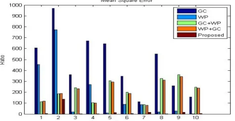
Graph 4.1 has revealed the comparative analysis of the Mean Square Error. The proposed algorithm is showing the better results than the available methods as mean square error is less in every case.

Figure 4.1 Comparative Analysis of MSE

Graph 4.2 is viewing the comparative analysis of the Root Mean Square Error. It has clearly demonstrated that the root mean square error is quite less in the case of the proposed algorithm; therefore proposed algorithm is providing better results.

Graph 4.3 has clearly demonstrated that the Normalized Absolute Error is quite less in the case of the proposed algorithm; therefore proposed algorithm is providing better results.

Figure 4.2 Comparative Analysis of RMSE

Figure 4.3 Comparative Analysis of NAE

Figure 4.4 Comparative Analysis of PSNR

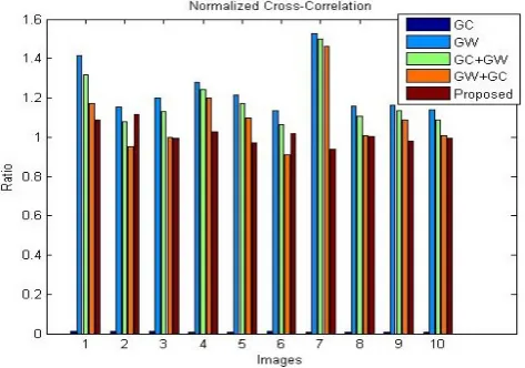
Graph 4.5 demonstrated the comparative analysis of the Normalized Cross-Correlation (NCC).Therefore proposed algorithm is showing better results than the available methods as NCC is close to 1 in every case.

Figure 4.5 Comparative Analysis of NCC

4.4. Comparative Analysis With Gray World Algorithm Using Graphs:

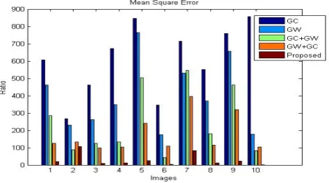
Graph 4.6 has shown the quantized analysis of the Mean Square Error. As mean square error need to be reduced therefore the proposed algorithm is showing the better results than the available methods as mean square error is less in every case.

Figure 4.6 Comparative Analysis of MSE

Graph 4.7 is demonstrated the comparative analysis of the Root Mean Square Error. It has visibly demonstrated that the root mean square error is quite less in the case of the proposed algorithm; therefore proposed algorithm is providing better results.

Figure 4.7 Comparative Analysis of RMSE

Graph 4.8 is showing the comparative analysis of the Normalized Absolute Error. It contains the average difference between input and output image. It has clearly demonstrated that the Mean Absolute Error is quite less in the case of the proposed algorithm; therefore proposed algorithm is providing better results.

Figure 4.8 Comparative Analysis of NAE

Graph 4.9 is viewing the comparative analysis of the Peak Signal to Noise Ratio (PSNR). As PSNR need to be maximized; so the main goal is to increase the PSNR as much as possible. It has clearly shown that the PSNR is maximum in the case of the proposed algorithm therefore proposed algorithm is providing better results than the available methods.

Figure 4.10 Comparative Analysis of NCC

Graph 4.10 shows the comparative analysis of the Normalized Cross-Correlation (NCC). As NCC needs to be close to 1, therefore proposed algorithm is showing better results than the available methods as NCC is close to 1 in every case.

5.CONCLUSION

This paper has proposed a new modified color constancy algorithm by integrating thegray world and white patch based color constancy algorithm withthe average filter, histogram stretching and the gamma correction. The review has shown that the existing methods may introduce some Gaussian noise and also degrade the effect of the brightness in the image. So average filter is used in this paper to remove the Gaussian noise and the histogram stretching is also used to improve the brightness of the image. The comparison of the proposed algorithm with other color constancy algorithms has shown the significant improvement over the available techniques.

In near future we will modify the gray world hypothesis by using the fuzzy if then rules to constant the colors in more efficient way.

REFERENCES

[1] Jing Yu, Qingmin Liao "Color Constancy-Based Visibility

Enhancement in Low-Light Conditions"

2010 Digital Image Computing: Techniques and Applications, IEEE 2010.

[2] Meng Wu, Jun Zhou, Jun Sun, Gengjian Xue "TEXTURE-BASED

COLOR CONSTANCY USING LOCAL REGRESSION" IEEE 2010.

[3] Arjan Gijsenij, Member, IEEE, and Theo Gevers, Member, IEEE

"Color Constancy Using Natural Image Statistics and Scene Semantics" IEEE 2011.

[4] Umasankar Kandaswamy, Donald A. Adjeroh, Member, IEEE,

"Robust Color Texture Features Under Varying Illumination Conditions" IEEE 2011.

[5] Seung-Kyun Kim, Seung-Won Jung, Kang-A Choi, Tae Moon Roh,

and Sung-Jea Ko, Senior Member, IEEE "A Novel Automatic White Balance for Image Stitching on Mobile Devices" IEEE 2011.

[6] Arjan Gijsenij, Member, IEEE, Rui Lu, and Theo Gevers, Member,

IEEE "Color Constancy for Multiple Light Sources" IEEE 2011.

[7] Lisa Brown, Ankur Datta, Sharathchandra Pankanti "Exploiting

Color Strength to Improve Color Correction" 2012 International Symposium on Multimedia , IEEE, 2012.

[8] Jonathan Cepeda-Negrete and Raul E. Sanchez-Yanez. "Combining

Color Constancy and Gamma Correction for Image Enhancement" 2012 Ninth Electronics, Robotics and Automotive Mechanics Conference , IEEE, 2012.

[9] Feng-Ju Chang and Soo-Chang Pei. "Color Constancy via

Chromaticity Neutralization:From Single to Multiple Illuminants" IEEE 2013.

[10] Hyunchan Ahn, Soobin Lee, and Hwang Soo Lee "improving the

color constancy by saturation weighting" IEEE 2013

[11] Li, Bing, Weihua Xiong, Weiming Hu, and OuWu. "Evaluating combinational color constancy methods on real-world images." In Computer Vision and Pattern Recognition (CVPR), IEEE, 2011.

[12] Arjan Gijsenij ,Theo Geversand Joost van de Weijer.

"Computational Color Constancy: Survey and Experiments" IEEE transaction on image processing, vol. 20, no. 9, september 2011.

[13] Su Wang, Yewei Zhang, Peng Deng, Fuqiang Zhou, “Fast Automatic

White Balancing Method by Color Histogram Stretching” IEEE 2011.

[14] Pengfei Luo, Min Zhang, Yile Liu, Dahai Han, Qing Li, "A Moving

Average Filter Based Method of Performance Improvement for Ultraviolet Communication System" IEEE 2012.

[15] EDWIN H. LAND* AND JOHN J. MCCANN,” Lightness and

Retinex Theory” Journal of the OPTICAL Of SOCIETY AMERICA.

[16] "Gamma Correction", [online available]:siggraph.org

[17] Richa Dogra, ArpinderSingh,"INTERNATIONAL JOURNAL OF