Joint Variable Selection of Mean Covariance Model for Longitudinal Data

Joint Variable Selection of Mean-Covariance

Model for Longitudinal Data

Dengke Xu1, Zhongzhan Zhang1, Liucang Wu1,2

1_{College of Applied Sciences, Beijing University of Technology, Beijing, China} 2_{Faculty of Science, Kunming University of Science and Technology, Kunming, China}

Email: [email protected]

Received October 23,2012; revised November 24, 2012; accepted December 9,2012

ABSTRACT

In this paper we reparameterize covariance structures in longitudinal data analysis through the modified Cholesky de- composition of itself. Based on this modified Cholesky decomposition, the within-subject covariance matrix is decom- posed into a unit lower triangular matrix involving moving average coefficients and a diagonal matrix involving inno- vation variances, which are modeled as linear functions of covariates. Then, we propose a penalized maximum likeli- hood method for variable selection in joint mean and covariance models based on this decomposition. Under certain regularity conditions, we establish the consistency and asymptotic normality of the penalized maximum likelihood es- timators of parameters in the models. Simulation studies are undertaken to assess the finite sample performance of the proposed variable selection procedure.

Keywords: Joint Mean and Covariance Models; Variable Selection; Cholesky Decomposition; Longitudinal Data;

Penalized Maximum Likelihood Method

1. Introduction

In recent years, the method of joint modeling of mean and covariance on the general linear model with multi- variate normal errors, was heuristically introduced by Pourahmadi [1,2]. The key advantages of such models include the convenience in statistical interpretation and computational ease in parameter estimation, which is described in Section 2. On the other hand, the estimation of the covariance matrix is important in a longitudinal study. A good estimator for the covariance can improve the efficiency of the regression coefficients. Furthermore, the covariance estimation itself is also of interest [3]. A number of authors have studied the problem of estimat- ing the covariance matrix. Pourahmadi [1,2] considered generalized linear models for the components of the modified Cholesky decomposition of the covariance ma- trix. Fan et al. [4] and Fan and Wu [5] proposed to use a semiparametric model for the covariance function. Re- cently, Rothman et al. [6] proposed a new regression in- terpretation of the Cholesky factor of the covariance ma- trix by parameterizing itself and guaranteed the positive- definiteness of the estimated covariance at no additional computational cost. Furthermore, based on this decom- position [6], Zhang and Leng [7] proposed efficient maximum likelihood estimates for joint mean-covariance analysis.

As is well known, as a part of modeling strategy, variable selection is an important topic in most statistical analysis, and has been extensively explored over the last three decades. In a traditional linear regression setting, many selection criteria (e.g., AIC and BIC) have been extensively used in practice. Nevertheless, those selec- tion methods suffer from expensive computational costs. As computational efficiency is more desirable in many situations, various shrinkage methods have been devel- oped, which include but are not limited to: the nonnega- tive garrotte [8], the LASSO [9], the bridge regression [10], the SCAD [11], and the one-step sparse estimator [12]. Recently, Zhang and Wang [13] proposed a new criterion, named PICa, to simultaneously select explana- tory variables in the mean model and variance model in heteroscedastic linear models based on the model struc- ture. Zhao and Xue [14] presented a variable selection procedure by using basis function approximations and a partial group SCAD penalty for semiparametric varying coefficient partially linear models with longitudinal data.

efficient penalized likelihood based method to select important explanatory variables that make a significant contribution to the joint modelling of mean and covari- ance structures for longitudinal data. With proper choices of the penalty functions and the tuning parameters, we establish the consistency and asymptotic normality of the resulting estimator. Simulation studies are used to illus- trate the proposed methodologies. Compared with exist- ing methods, our procedure offers the following differ- ences and improvements. Firstly, Zhang and Leng [7] discussed efficient maximum likelihood estimates and model selection for joint mean-covariance analysis based BIC. As is well known, BIC selection method would suffer from expensive computational costs. However, our method can select significant variables and obtain the parameter estimators simultaneously in the joint model- ling of mean and covariance structures for longitudinal data, that implies that our method can avoid the heavy computational burden. Secondly, in this paper we assume the covariates may be of high dimension, which become increasingly common in many health studies, and our method also can select the important subsets of the cova- tiates. Thirdly, we reparameterize covariance structures in longitudinal data analysis through the modified Cho- lesky decomposition of itself, which is brought closer to time series analysis, for which the moving average model may provide an alternative, equally powerful and parsi- monious representation.





T

1, , i

i i im

    



mi1



vector and i

The rest of this paper is organized as follows. In Sec- tion 2 we first describe a reparameterization of covari- ance matrix itself through the modified Cholesky de- composition and introduce the joint mean and covariance models for longitudinal data. We then propose a variable selection method for the joint models via penalized like- lihood function. Asymptotic properties of the resulting estimators are considered in Section 3. In Section 4 we give the computation of the penalized likelihood estima- tor as well as the choice of the tuning parameters. In Sec- tion 5 we carry out simulation studies to assess the finite sample performance of the method.

2. Variable Selection for Joint

Mean-Covariance Model

2.1. Modified Cholesky Decomposition of the Covariance Matrix

Suppose that there are n independent subjects and the ith

subject has mi repeated measurements. Specifically, de-

note the response vector



₁, ,



T

i

i i im

y y  y







T

1, , i

i i im

t t  t



1, ,

i  n

for the ith

subject, , which are observed at time

 . We assume that the response vector is

normally distributed as

is an  is an



m m



i1, , n



1

i i positive definite matrix



. As a

tool for regularizing the inverse covariance matrix, Pourahmadi [1] suggested using the modified Cholesky

factorization of i



 . To parametrize , Pourahmadi

[1] first proposed to decompose it as i i i i. The

lower triangular matrix i is unique with 1’s on its di-

agonal and the below diagonal entries of Ti are the

negative autoregressive parameters

i 

T T T D T

ijk

 in the model





1 1

j

ij ij ijk ik ik ij

k

y  y  

 





 

i D

.



The diagonal entries of are the innovation vari-

ances as 2 _Var

 

ij ij





~ ,

i i i

y N   , where

  

1 L T

T T D T  

l L

1 1

, 2, ,

j

ij ij ijk ik ij i

k .

According to the idea of the proposed decomposition

in Rothman et al. [6], we let i i , a lower triangular

matrix with 1’s on its diagonal, we can write

i i i i . We actually use a new statistically mean-

ingful representation that reparameterizes the covariance matrices by the modified Cholesky decomposition advo-

cated by Rothman et al. [6]. The entries ijk in i can

be interpreted as the moving average coefficients in

y  l   j m

 

 



  

1 1 1

i yi i

,

where    and i N



0,Di



for





T

1, , _i

i i im

     . Note that the parameters l_ijk and

 

2

log _ij are unconstrained.

Based on the modified Cholesky decomposition and motivated by [1,2] and Ye and Pan [15], the uncon-

strained parameters ij,lijk and

 

ij

2

log  are modeled

in terms of the generalized linear regression models (JMVGLRM)



T _, T _{, log}

 

2 T

ij ij ijk ijk ij ij



g  x  l z   h . (1)

 

g

Here  is a monotone and differentiable known

link function, and xij, ijk and ij are the p × 1, q × 1

and d × 1 vectors of covariates, respectively. The covari-

ate ij

z h

x and ij are the usual covariates used in regres-

sion analysis, while ijk is usually taken as a polyno-

mial of time difference h

z

ik ij

t t . In addition, denote





T

1, , i

i i im

X  x  x and Hi 



hi1, , himi



T. We further

refer to  as moving average coefficients and  as

innovation coefficients. In this paper we assume that the

covariates xij, ijk and ij may be of high dimension

and we would select the important subsets of the covari-

ates ij

z h

x , ijk and ij, simultaneously. We first assume

all the explanatory variables of interest, and perhaps their interactions as well, are already included into the initial models. Then, we aim to remove the unnecessary ex- planatory variables from the models.

2.2. Penalized Maximum Likelihood for JMVGLRM

Many traditional variable selection criteria can be con- sidered as a penalized likelihood which balances model-

ling biases and estimation variances [11]. Let 

 



denote the log-likelihood function. For the JMVGLRM, we propose the penalized likelihood function

   

 

 

 2

 

 3

 

1 1

p

i

d

j k

j k

p p

 



1 1

i q

L p



 

 

 









T

T

1  q; , ,1 d



 

 





(2)

where 



₁, ,_s



 ₁, ,  _p; , ,

with s  p q d and p_{ }l

 



 l

 is a given penalty

function with the tuning parameter . The

tuning parameters can be chosen by a data-driven crite- rion such as cross validation (CV), generalized cross- validation (GCV) [9], or the BIC-type tuning parameter selector [16] which is described in Section 4. Here we

use the same penalty function for all the regres-

sion coefficients but with different tuning parameters



l 1, 2,3



 

 

p 

 1

 , _ 2 _{and } 3 _{for the mean parameters, moving}

average parameters and log-innovation variances, respec- tively. Note that the penalty functions and tuning pa- rameters are not necessarily the same for all the parame- ters. For example, we wish to keep some important vari- ables in the final model and therefore do not want to pe- nalize their coefficients. In this paper, we use the smoothly clipped absolute deviation (SCAD) penalty whose first derivative satisfies

 



 

_

_



I t





1

a t

p I t

a





  

   _  

  

  _

 

 

2

a

3.7

a

for some [11]. Following the convention in [11],

we set in our work. The SCAD penalty is a

spline function on an interval near zero and constant out- side, so that it can shrink small value of an estimate to zero while having no impact on a large one.

The penalized maximum likelihood estimator of ,

denoted by ˆ, maximizes the function L

 

 in (2).

With appropriate penalty functions, maximizing L

 



with respect to  leads to certain parameter estimators

vanishing from the initial models so that the correspond- ing explanatory variables are automatically removed.

Hence, through maximizing L

 

 we achieve the goal

of selecting important variables and obtaining the pa- rameter estimators, simultaneously. In Section 4, we pro- vide the technical details and an algorithm for calculating

the penalized maximum likelihood estimator ˆ.

3. Asymptotic Properties

We next study the asymptotic properties of the resulting

penalized likelihood estimate. We first introduce some

notations. Let 0 denote the true values of . Fur-

thermore, let





_T

 

 ₁ T

 

 ₂ T T 0 01, , 0s 0 , 0

    _{ }   _

 



 1

.

For ease of presentation and without loss of generality,

it is assumed that 0 consists of all nonzero compo-

nents of  2

0 0



0

 and that  . Denote the dimension of

 1 0

 by s1. Let

 



0 0



1

max _n : 0

n j j

j s

a p_  

  

 

and



 

0 0



1

max : 0

n

n j j

j s

b p_  

   .

 

 l

Here we denote  as n to emphasize its de-

pendence on sample size . n

 1

n  is equal to either  ,

 2

 or _3_{, depending on whether}

j 0

 is a component

of ₀, ₀ or ₀



1 j s



,

.

To obtain the asymptotic properties in the paper, we require the following regularity conditions:

(C1): The covariate vectors x zij ijk

i m

and hij are fixed.

Also, for each subject the number of repeated measure-

ments, , is fixed



i1, , , n j1, , m ki, 1, , j1



.

(C2): The parameter space is compact and the true

value ₀ is in the interior of the parameter space.

(C3): The design matrices Xi and Hi in the joint

models are all bounded, meaning that all the elements of the matrices are bounded by a single finite real number.

Theorem 1 Assume a O

 

n1 2 b 0

0 n p

, n and

n

  n 

ˆ

as . Under the conditions (C1)-(C3),

with probability tending to 1 there must exist a local

maximizer _n of the penalized likelihood function

ˆ

n

 

L  in (2) such that  is a n-consistent estimator

of ₀.

The following theorem gives the asymptotic normality property of ˆ_n. Let



 

 

 

 



1

1 1

01 0

diag , ,

n n

n s

A  p_   p_ 

 



 

 

 

 

 

 

 



1 1

T

1 1

1 1

01 sgn 01 , , 0 sgn 0 ,

n n

n s s

c  p_    p_  

 1

where 0j is the jth component of .

 1

_

₁

_

j s

  

 _{0 1}

Denote the Fisher information matrix of  by In

 

 .

 

Theorem 2 Assume that the penalty function p_n t

 

satisfies

0

lim inf liminf n 0

n t

n

p_ t

 

 

 

 

definite matrix I



0



as . Under the same mild

conditions as these given in Theorem 1, if n

n 

0

  and

n

n   as n , then the n -consistent esti-

mator in Theorem 1 must sat-

isfy

 

 

1

ˆ ˆ _,

n n

  

0

 

 

_ˆ T

T ₂ T

n      

1) ˆn 2 with probability tending to 1.

2)

 

 1 1 2



 1







 1  1





 1



1



0

ˆ

n n n n n n n

n I  I     I A  c

 

1 0, 1

A L s s N I  L  ,

where “” stands for the convergence in distribu-

tion; In 1 is the



s1s1



submatrix of In corre-

sponding to the nonzero components 0 1 and Is1 is

the



s1s1



 

L

identity matrix.

Remark: The proofs of the Theorems 1 and 2 are simi- lar to [11]. To save space, the proofs are omitted.

4. Computation

4.1. Algorithm

Because  is irregular at the origin, the commonly

used gradient method is not applicable. Now, we develop an iterative algorithm based on the local quadratic ap-

proximation of the penalty function p

 

 as in [11].





Firstly, note the first two derivatives of the log-likeli-

hood function  



are continuous. Around a given

point 0, the log-likelihood function can be approxi-

mated by

   

  







  



0 0

0

0 T 0 .

   T 0 2 T 1 2               _       _{ }          t     

 

t

Also, given an initial value 0we can approximate the

penalty function p_ by a quadratic function [11]

 

 

 

0



2 2



0 0 0 1 , 2 p t

p t t t

t



 





tt

p t

 

for 0.

Therefore, the penalized likelihood function (2) can be local approximated, apart from a constant term, by

   

  







  



T

 

0 ,  T 0 0 0 2 T 0

0 T 0

1 2 2 L n                _{ }                          

 

  where

 

 

 

 

 

 

 

 

 

 





1 1 2

1 1

3 3

2

1

01 0 01

0

01 0 01

0 01

0

0 01 0

diag , , , ,

, , , , , | | | | p q d p p d q q d

p p p

p p p                            _            





where





T

T

1, , s 1, , p, , , , , ,1 q 1 d

            









T

0 01 0

T

01 0 01 0 01 0

, ,

, , , , , , , , .

s

p q d

               and

Accordingly, the quadratic maximization problem for

 

L  leads to a solution iterated by

 

_{ }

1

_{ }

 

2

0 0

1 0 T n  0 n  0 0 .

                     _   _{ }   _             

Secondly, as the data are normally distributed the

log-likelihood function 

 



 

can be written as

 









 

T 1 1 1 T 1 1 1

1 _log 1

2 2

1 1

log .

2 2

n n

i i i i i i

i i

n n

i i i i

i i y y D D                     











 

Therefore, the resulting score functions are

 

_

_T

_{ }

_T

_{ }

_T

_{ }

_

T

1 , 2 , 3 ,

U   U  U  U 

     

 

where

 

T 1

_

_

_

_

1

1

;

n

i i i i i i i

U   X y  X

  



    







 

 

T 1 2 1 ; n i i i i

U    D 

   

 

  









 

 

T



1



3

1

1 _{1 .}

2 i

n

i i i m i

U   H D f

  



  













1

 

T 1



T





1

diag , , _i

i i Xi g xi g xim

Here           ,

 

1

g  is the derivative of the inverse of the link func-

tion 1

 



g  , and i  i1, ,im_i



T





1 _T 1 1 ; , , i j

ij ij ijk ik i i im

k

r l f f f

     



  2 ij ij f with

 

 

 

 

 

 

 

 

 

 

 

2 T

2 2 2

T T

2 2 2

T T

2 2 2

T T

11 12 13 21 22 23 31 32 33

,

n

I E

E E E

E E E

E E E

I I I

I I I

I I I

    T T T                                                             _{   }                          _    _                

T 1 _;

i i i i i

where

11 1

n

i

I  X    X





T 1 _; i i i D 22 1 n i

I E  

        



T 1 1 2 n i i i 33

I H H







0.

I I I I 

0

and _{12 21 13 31 23 32}

Finally, by using the Fisher information matrix to ap- proximate the observed information matrix, the following algorithm summarizes the computation of penalized maximum likelihood estimators of the parameters in JMVGLRM.

I I 

Algorithm:

Step 1. Take the ordinary maximum likelihood esti-

mators (without penalty)  , ₀, ₀ of , ,  as

their initial values.

Step 2. Given the current values  m  m

 



 T_, mT_, mT



T

 

 



 

 

 



1 . m

m m m

          

 

p 



1, 2,3





 i,i 1, , s



 

update it by

   



 

 

 

 



1

m m m

n

I n

U n 

  _ _ 

 

Step 3. Repeat Step 2 above until certain convergence criteria are satisfied.

4.2. Choosing the Tuning Parameters

The penalty function _l involves the tuning pa-

rameters that controls the amount of

penalty. Many selection criteria, such as CV, GCV, AIC and BIC selection can be used to select the tuning pa- rameters. Wang et al. [16] suggested using the BIC for the SCAD estimator in linear models and partially linear

models, and proved its model selection consistency prop- erty, i.e., the optimal parameter chosen by BIC can iden- tify the true model with probability tending to one. Hence, we use their suggestion throughout this paper. So the

BIC will be used to choose the optimal

 l

l

 



which is equal to either 1_{, 1, ,}



i i p

  

 

,



2_{, 1, ,}



j j q

  



 3_{, 1, ,}



k k d

   . Nevertheless, in

or

real application, how to simultaneously select a total of s

shrinkage parameters



 ,i 1, , s



 

i is challenging. To

bypass this difficulty, we follow the idea of [12,16,17], and simplify the tuning parameters as

1) 1

1i ₀ , 1, , , i i p         

2) 2

2j ₀ , 1, , , j j q         

3) 3

3k ₀ , 1, , k k d       

 0

in the numerical studies followed, where i

 0

, _j

 0 and

k



0

are respectively the ith element, jth element and kth

element of the unpenalized estimate  _{, }0 _{and }0

i

. Consequently, the original s dimensional problem about

 becomes a three dimensional problem about

1 2 3





T

, , .

    can be selected according to the fol-

lowing BIC-type criterion





log

 

2 _{ˆ ˆ ˆ}

BIC , , df n

n n

        

0 df_ s

.



ˆ is simply the number of nonzero co-

where 

. efficients of

From our simulation study, we found that this method works well.

5. Simulation Studies

In this section we conduct simulation studies to assess the small sample performance of the proposed proce- dures. We consider the sample size n = 100, 200, and 400 respectively. Each subject is supposed to be measured by

i times with i . In the simu-

lation study, 1000 repetitions of random samples are generated by using the above data generation procedure. For each simulated data set, the proposed variable selec- tion procedures for finding out penalized maximum like- lihood estimators with SCAD and adaptive lasso (ALASSO) penalty functions [17] are considered. The unknown tuning parameters

m m 1 Binomial 11,0.8





 l

 , for the

penalty functions are chosen by BIC criterion in the simulation. The performance of estimator



l1, 2,3



ˆ _ˆ

 ,  and

ˆ

 will be assessed by the mean square error (MSE),



 

T



0 ˆ 0 ,

 

ˆ ˆ

MSE  E    



 

T



0 ˆ 0 ,

ˆ ˆ

MSE( ) E    



 

T



0 ˆ 0

ˆ ˆ

MSE( ) E     .





T 1, 2 , 10

   ，  1 1

5.1. Example 1: Linear Mean Model for JMVGLRM

In this example, we first consider the linear model for mean parameters as a special JMVGLRM. We choose the true values of the mean parameters, moving average parameters and log-innovation variances to be

with   , 2 0.5, 40.5,





T 7

,

1, ,2

     with 20.5, 30.4, and





T

,

1, ,2 7

      with 1 0.3, 20.3, respec-

tively, while the remaining coefficients, corresponding to the irrelevant variables, are given by zeros. In the models



_T



T 1

1,

ij ij

x  x with x1ij is generated from a multivariate

normal distribution with mean zero, marginal variance 1

and all correlations 0.5. We take

 

7 and

1 ij ijt _t

h  x _







T

2 6

, tijtik







,

t t t





1,   ,

ijk ij ik ij ik

z t 

t

and the measurement times ij are generated from the

uniform distribution U 0, 2



. Using these values, the

mean i and covariance matrix i are constructed

through the modified Cholesky decomposition described

in Section 2. The responses i are then drawn from the

multivariate normal distribution y



,



, 1, , .

N   i  n

ˆ

i i

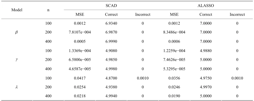
The average number of the estimated zero coefficients for the parametric components, with 1000 simulation

runs, is reported in Table 1. Note that “Correct” in Table

1 means the average number of zero regression coeffi-

cients that are correctly estimated as zero, and “Incor- rect” depicts the average number of non-zero regression coefficients that are erroneously set to zero.

From Table 1, we can make the following observa-

tions. Firstly, the performances of variable selection pro- cedures with different penalty functions become better and better as n increases. For example, the values in the column labeled “Correct” become more and more closer to the true number of zero regression coefficients in the models. Secondly, the SCAD and ALASSO penalty methods perform similarly in the sense of correct vari- able selection rate, which significantly reduces the model uncertainty and complexity. Thirdly, for the designed settings, the overall performance of the variable selection procedure is satisfactory.

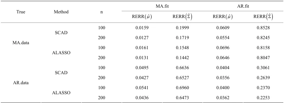
Next, we compare the two decomposition methods under two data generating processes, autoregressive (AR) decomposition [1] and moving average (MA) decompo- sition [6]. The main measurements for comparison are

differences between the fitted mean i and the true

mean i, and the fitted covariance matrix ˆi to the

true i. In particular, we define two relative errors as

 

 

1 1

ˆ ˆ

1 _ˆ 1

ˆ

RERR n i i , RERR n i i .

i i i i

n n

  



 

   

  







Here A denotes the largest singular value of A. We

compute the averages of these two relative errors for

1000 replications with n = 100 and 200. Table 2 gives

the averages of relative errors for the MA decomposition and AR decomposition, when the data are generated from

our model under different true covariance matrix. In Ta-

ble 2, “MA.data” (“AR.data”) means that the true co-

[image:6.595.56.539.541.734.2]

variance matrix follows the moving average structure (autoregressive structure). “MA.fit” (“AR.fit”) means we

Table 1. Variable selection for JMVGLRM (linear mean model) using different penalties and sample size.

SCAD ALASSO Model n

MSE Correct Incorrect MSE Correct Incorrect

100 0.0012 6.9340 0 0.0012 7.0000 0

200 7.8107e−004 6.9870 0 8.3486e−004 7.0000 0



400 0.0005 6.9990 0 0.0006 7.0000 0

100 1.3369e−004 4.9080 0 1.2259e−004 4.9880 0

200 6.5800e−005 4.9850 0 7.4626e−005 5.0000 0



400 4.6587e−005 4.9980 0 5.3295e−005 5.0000 0

100 0.0417 4.8700 0.0010 0.0356 4.9750 0.0010

200 0.0254 4.9380 0 0.0246 4.9970 0



[image:7.595.57.538.100.275.2]

Table 2. Average of relative errors using different methods and sample size.

MA.fit AR.fit True Method n

 ˆ

RERR  _RERR

 

_ˆ _{RERR ˆ RERR}

 

_ˆ

100 0.0159 0.1999 0.0609 0.8528 SCAD

200 0.0127 0.1719 0.0554 0.8245 100 0.0161 0.1548 0.0696 0.8158 MA.data

ALASSO

200 0.0131 0.1442 0.0646 0.8047 100 0.0495 0.6636 0.0404 0.3061 SCAD

200 0.0427 0.6527 0.0356 0.2639 100 0.0541 0.6960 0.0400 0.2370 AR.data

ALASSO

200 0.0436 0.6473 0.0362 0.2253

decompose the covariance matrix by MA decomposition (AR decomposition) to fit data. We see that when the true covariance matrix follows the moving average

structure, the errors in estimating  and both in-

crease when incorrectly decomposing the covariance matrix using the autoregressive structure, and vice versa. However, for this simulation study, model misspecifica- tion seems to affect the MA decomposition less than AR decomposition.



 

T ij ij

it x

5.2. Example 2: Generalized Linear Mean Model for JMVGLRM

Consider the following logistic link function to model the mean component in the JMVGLRM, then we have

log   

 

T T

 

2 T 0, ij hij

.

We use the settings in example 1 to assess the per- formance of the proposed variable selection procedures,

and the simulation results are reported in Table 3.

The results in Table 3 show that under different sam-

ple size, the proposed variable selection methods have the desired performance, which is substantively similar to the previous example.

5.3. Example 3: High-Dimensional Setup for JMVGLRM

In this example, we discuss how the proposed variable selection procedures can be applied to the “large n, di-

verging s” setup for JMVGLRM. We consider the fol-

lowing high-dimensional logistic mean model in JMVGLRM:

0 0

logit ij xij ,lijk zijk , log   

where 0 is a p-dimensional vector of parameters with

1 3

4 4

p_ n _ for n = 100, 200 and 400, and  u

0

 is a q-dimensional vector of parameters with



denotes the largest integer not greater than u. In addition,

1 3

2 2

q_ n _ and 0 is a d-dimensional vector of

parameters with 1 3



T



T

1

3 3 ij 1, ij

d_ n _ x  x with x1ij

is generated from a multivariate normal distribution with mean zero, marginal variance 1 and all correlations 0.5. We take

 

d₁ ij ijt _t

h  x _











_{2 1}



T

1, , , , q

ijk ij ik ij ik ij ik

z  t t t t  t t 

ij

t

,

where the measurement times are generated from the

uniform distribution U

 

0, 2 .

The true coefficient vectors are





T

0 1, 0.5,0.5,0p3

  - 





T

0 0.4, 0.4,0d 2

  -  _





T

0 0.6,0.6,0q 2 ,

  - _

0

and, where m denotes a m-vector of 0’s. Using these

values, the mean i and covariance matrix i are

constructed through the modified Cholesky decomposi-

tion described in Section 2. Then, the responses i are

then drawn from the multivariate normal distribution y



,



, 1, , .

N   i  n

11261025); Funding Project of Science and Technology

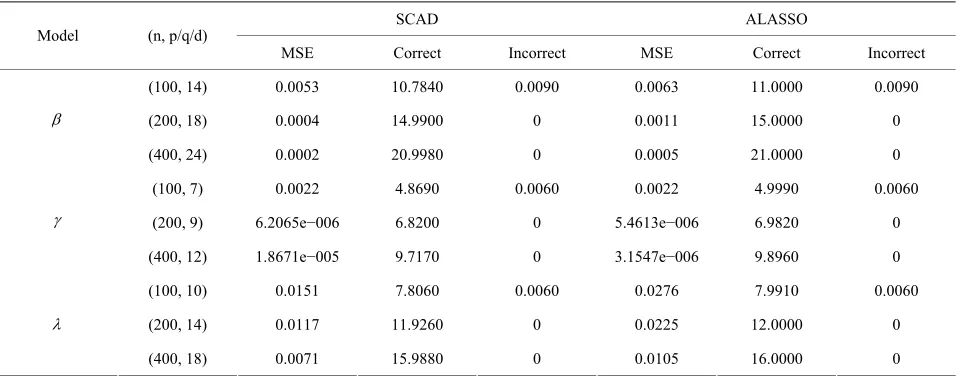
i i The summary of simulation re-

sults are reported in Table 4.

It is easy to see from Table 4 that, the proposed vari-

able selection method is able to correctly identify the true submodel, and works remarkably well, even if it is the “large n, diverging s” setup for JMVGLRM.

6. Acknowledgements

[image:8.595.58.538.102.291.2]

Table 3. Variable selection for JMVGLRM (generalized linear mean model) using different penalties and sample size.

SCAD ALASSO Model n

MSE Correct Incorrect MSE Correct Incorrect

100 0.1346 6.8820 0.0300 0.1591 6.9580 0.0700

200 0.1028 6.9920 0 0.0886 6.9980 0.0010



04 4.8480 1.4948e 04 4.9900

400 0.0838 7.0000 0 0.0727 7.0000 0

100 1.2997e−0 0 −0 0

200 7.2503e−005 4.9720 0 8.3386e−005 5.0000 0

0.0030

400 2.5737e−005 4.9820 0 5.9863e−005 5.0000 0

100 0.0149 4.9270 0 0.0297 4.9980

200 0.0086 4.9940 0 0.0178 5.0000 0



400 0.0059 5.0000 0 0.0135 5.0000 0



able 4. Variable selection for high-dimensional JMVGLRM (generalized linear mean model) using different penalties and

SCAD ALASSO

T

sample size.

Model (n, p/q/d)

MSE Correct Incorrect MSE Correct Incorrect

(100, 14) 0.0053 10.7840 0.0090 0.0063 11.0000 0.0090

(200, 18) 0.0004 14.9900 0 0.0011 15.0000 0



0.0060 0.0022

6.2065e 06 6.8200 5.4613e 06 6.9820

(400, 24) 0.0002 20.9980 0 0.0005 21.0000 0

(100, 7) 0.0022 4.8690 4.9990 0.0060

(200, 9) −0 0 −0 0

(

0.0060 0.0276

11.926 12.000

400, 12) 1.8671e−005 9.7170 0 3.1547e−006 9.8960 0

(100, 10) 0.0151 7.8060 7.9910 0.0060

(200, 14) 0.0117 0 0 0.0225 0 0



(400, 18) 0.0071 15.9880 0 0.0105 16.0000 0



esearch Plan of Beijing Education Committee (JC-

[1] M. Pourahma ance Models with

R

006790201001); Beijing municipal key disciplines (No. 006000541212010).

REFERENCES

di, “Joint Mean-Covari

Applications to Lontidinal Data: Unconstrained Parame- terisation,” Biometrika, Vol. 86, No. 3, 1999, pp. 677- 690. doi:10.1093/biomet/86.3.677

[2] M. Pourahmadi, “Maximum Likelihood Estimation for Generalised Linear Models for Multivariate Normal Co- variance Matrix,” Biometrika, Vol. 87, No. 2, 2000, pp. 425-435. doi:10.1093/biomet/87.2.425

[3] P. T. Diggle and A. Verbyla, “Nonparametric Estimation of Covariance Structure in Longitudinal Data,” Biomet- rics, Vol. 54, No. 2, 1998, pp. 401-415.

doi:10.2307/3109751

Data with Semiparam

[4] J. Q. Fan, T. Huang and R. Li, “Analysis of Longitudinal etric Estimation of Covariance Function,” Journal of the American Statistical Associa- tion, Vol. 102, No. 478, 2007, pp. 632-641.

doi:10.1198/016214507000000095

[5] J. Q. Fan and Y. Wu, “Semiparametric E

Covariance Matrices for Longitudinal Data,” stimation of Journal of the American Statistical Association, Vol. 103, No. 484, 2008, pp. 1520-1533. doi:10.1198/016214508000000742

[6] A. J. Rothman, E. Levina and J. Zhu, “A New Approach to Cholesky-Based Covariance Regularization in High Dimensions,” Biometrika, Vol. 97, No. 3, 2010, pp. 539- 550. doi:10.1093/biomet/asq022

[7] W. P. Zhang and C. L. Leng, “A Moving Average Cho- lesky Factor Model in Covariance Modeling for Longitu- dinal Data,” Biometrika, Vol. 99, No. 1, 2012, pp. 141- 150. doi:10.1093/biomet/asr068

[image:8.595.59.538.329.517.2]

384. doi:10.1080/00401706.1995.10484371

[9] R. Tibshirani, “Regression Shrinkage and Selection via the LASSO,” Journal of Royal Statistical Society,

nd Graphical Sta-

perties,” Journal Series B, Vol. 58, No. 1, 1996, pp. 267-288.

[10] W. J. Fu, “Penalized Regression: The Bridge versus the LASSO,” Journal of Computational a

tistics, Vol. 7, No. 3, 1998, pp.397-416.

[11] J. Q. Fan and R. Li, “Variable Selection via Nonconcave Penalized Likelihood and Its Oracle Pro

of American Statistical Association, Vol. 96, No. 456, 2001, pp. 1348-1360. doi:10.1198/016214501753382273

[12] H. Zou and R. Li, “One-Step Sparse Estimates in Non- concave Penalized Likelihood Models,” The Annals of Statistics, Vol. 36, No. 4, 2008, pp. 1509-1533.

doi:10.1214/009053607000000802

[13] Z. Z. Zhang and D. R. Wang, “Simultaneous Selection for Heteroscedastic Regr

Va ession Models,”

Sci-riable ence China Mathematic, Vol. 54, No. 3, 2011, pp. 515-

530. doi:10.1007/s11425-010-4147-8

[14] P. X. Zhao and L. G. Xue, “Variable Selection in Semi-

2-7

parametric Regression Analysis for Longitudinal Data,” Annals of the Institute of Statistical Mathematics, Vol. 64, No. 1, 2012, pp. 213-231.

doi:10.1007/s10463-010-031

ng of Covariance Struc- [15] H. J. Ye and J. X. Pan, “Modelli

tures in Generalized Estimating Equations for Longitudi- nal Data,” Biometrika, Vol. 93, No. 4, 2006, pp. 927-941.

doi:10.1093/biomet/93.4.927

[16] H. Wang, G. Li and C. L. Tsai, “Tuning Parameter Se- lectors for the Smoothly Clipped Absolute Deviation Me- thod,” Biometrika, Vol. 94, No. 3, 2007, pp. 553-568.

doi:10.1093/biomet/asm053

[17] H. Zou, “The Adaptive Lasso and Its Oracle Properties,”

00735

Journal of American Statistical Association, Vol. 101, No. 476, 2006, pp. 1418-1429.