ABSTRACT
COMBS, DUSTIN CLARK. Beta Decay as a Test of the Standard Model. (Under the direction of Albert Young.)
Measured observables from theβdecay of nuclei can be used to determineVu d, the first element
in the Cabibbo-Kobayashi-Maskawa (CKM)quark mixing matrix. If there are only three generations
of quarks, as predicted in the standard model, then the current 3x3 matrix would be unitary. Unitarity
can be checked by summing the squares of any of the rows or columns. The first row is known with
the greatest precision and provides the strictest test of unitarity. Of the elements in the first row,
the elementVu d is the largest and as a consequence, bears the most experimental scrutiny. The most precise determination ofVu d comes from the "superallowed", purely vector 0+→0+decays.
Mirror decays which have both vector and axial-vector components provide an independent check
on the unitarity of the CKM matrix as well as checks on the calculated corrections that are applied
to both types of decays. A new analysis of the unpublished results of aβ asymmetry measurement
of the mirror decay nuclei19Ne performed at Princeton University in 1994 was undertaken. The asymmetry value is found with an uncertainty of 2.4%. This value and the current world average
for the lifetime of the decay are used to extractVu dwith an uncertainty of 0.2%, the most precise
determination from a mirror nuclei decay.
The observation of neutrinoless double beta decay would provide proof of the existence of
Ma-jorana leptons. A measured half-life for the decay when used in conjunction with the nuclear matrix
element would yield an effective Majorana mass for the neutrino. The only method for obtaining
the nuclear matrix element, aside from the measurement of the decay itself, is computational. The
two most commonly used means of undertaking the computation use the shell model or the quasi
random phase approximation (QRPA). The QRPA method relies on the Bardeen-Cooper-Schriff
(BCS) theory to describe the ground state of the initial and final nuclei. The validity of the BCS
description of the ground state can be tested experimentally with two nucleon transfer reactions. If
from a two nucleon transfer reaction should be suppressed by a factor ofA/4 relative to the ground state. The cross sections for the two proton transfer reaction (3He,n) on the double beta decay isotopes128Te and130Te were measured at 0◦with a systematic uncertainty of 8.6% and statistical uncertainties of 7.3% and 7.5%, respectively. These are the most precise measurements of these
© Copyright 2018 by Dustin Clark Combs
Beta Decay as a Test of the Standard Model
by
Dustin Clark Combs
A dissertation submitted to the Graduate Faculty of North Carolina State University
in partial fulfillment of the requirements for the Degree of
Doctor of Philosophy
Physics
Raleigh, North Carolina
2018
APPROVED BY:
Paul Huffman Dean Lee
Gail McLaughlin Albert Young
DEDICATION
ACKNOWLEDGEMENTS
I’d like to thank my fellow graduate student and co-conspirator, David Ticehurst. Our approaches in
the lab were wildly different. I was the cautious and reserved member of the duo while David liked
to jump in with both feet. I truly admire his fearlessness. David also kept the control room supplied
with snacks during long shifts. David is responsible for much of the text in Chapter 4 particularly
the section describing the ion source. I’d also like to thank David’s mom Lynne Ticehurst, who
brought many meals to the lab. Brent Fallin, Forrest Freisen and Ron Malone are forever in my debt
for the numerous shifts that they took so that David and I could get some sleep. Robert Pattie was
already a grizzled veteran when I joined Dr. Young’s group at NCSU. He taught me a lot about Monte
Carlo simulations in general and the use ofPENELOPEin particular. I appreciated the entertaining
conversations and the overall esprit de corps from my numerous officemates over the years.
The measurements at TUNL would not have been possible without the help and guidance of
the technical staff. Richard O’Quinn was an invaluable source of knowledge about the tandem
accelerator. John Dunham was a huge help in constructing and leak testing the helium recirculation
system. He also taught me how to service and operate the helium ion source. The placement of the
neutron detectors in the target room as well as surveying the 70 degree beam line was undertaken
with a great deal of assistance from Mark Emamian. Bret Carlin provided support in setting up the
data acquisition system and in establishing controls for the source and recirculation sytem. Chris
Westerfeldt procured the parts for the recirculation system and many other items necessary for the
construction of the experiment. He was also an incredible resource for help in finding or fixing just
about anything in the lab.
I’d like to thank my advisor, Albert Young, for his patience and for treating me like a colleague
and not just a student. I am grateful to Gordon Jones for his assistance. It was his thesis data from
the Princeton19Ne experiment that I used in my analysis. Calvin Howell led much of the work at Duke. He was incredibly supportive and very generous with his time despite having considerable
getting the data acquisition system up and running. Tom Clegg was an excellent sounding board on
issues related to the helium source.
Finally, I’d like to thank my family. I can’t thank my parents enough for their love and support.
I’m grateful to my three boys, for reminding me what is truly important. The one person to whom I
owe the greatest debt of gratitude is my wife, Cari. Her encouragement kept me going during trying
TABLE OF CONTENTS
LIST OF TABLES . . . vii
LIST OF FIGURES. . . .viii
Chapter 1 Theory . . . 1
1.1 Beta Decay . . . 2
1.1.1 V-A Theory . . . 2
1.1.2 AllowedβDecay . . . 4
1.1.3 Cabibbo-Kobayashi-Maskawa Matrix . . . 5
1.1.4 Mixed Decays . . . 7
1.1.5 19Ne Decay . . . 9
1.2 Massive Neutrinos . . . 9
1.2.1 Neutrino Oscillation . . . 9
1.2.2 Dirac and Majorana Neutrinos . . . 12
1.3 Double Beta Decay . . . 13
1.3.1 Nuclear Matrix Element Calculations . . . 16
1.3.2 Motivation for Transfer Reactions . . . 19
Chapter 2 19Ne Decay Simulation . . . 22
2.1 The 1994 Princeton Experiment . . . 22
2.2 Simulation Model . . . 24
2.3 Construction of Detector Pulses . . . 26
2.4 χ2Minimization . . . 28
Chapter 3 Analysis of19Ne Decay . . . 33
3.1 Uncertainties . . . 33
3.2 Results . . . 41
3.3 Determination ofVu d. . . 42
Chapter 4 Two Proton Transfer Experimental Setup . . . 48
4.1 Alpha Source . . . 49
4.2 Beam Pulsing . . . 52
4.3 Tandem . . . 56
4.4 Beam Transport . . . 58
4.5 Pickoff Unit . . . 59
4.6 Detectors . . . 61
4.6.1 Liquid Scintillator Detectors . . . 61
4.6.2 CsF Detectors . . . 64
4.6.3 Surface Barrier Detectors . . . 64
4.7 Electronics and DAQ . . . 68
5.1 Design . . . 70
5.2 Performance . . . 73
5.3 Gas Contamination . . . 74
5.4 Operation and Maintenance . . . 75
5.5 Improvements . . . 77
Chapter 6 Target Fabrication . . . 79
6.1 Target Material . . . 79
6.2 Evaporator Operation . . . 81
6.3 Thickness Measurement . . . 85
Chapter 7 Neutron Detector Efficiencies . . . 89
7.1 Simulations . . . 90
7.2 Neutron Time of Flight . . . 91
7.2.1 Deuterium Data . . . 93
7.2.2 Tritium Data . . . 94
7.3 Comparison to Simulation . . . 97
7.4 Relative Efficiency . . . 99
7.5 Uncertainty . . . 99
Chapter 8 Analysis of Transfer Reaction . . . .101
8.1 TOF Spectra . . . 102
8.2 Cuts . . . 103
8.3 Data Sets . . . 105
8.4 128Te(3He,n)130Xe . . . 107
8.5 130Te(3He,n)132Xe . . . 109
8.6 Uncertainties . . . 112
8.7 Discussion of Results . . . 116
Chapter 9 Conclusions . . . .118
9.1 Beta Asymmetry Measurement . . . 118
9.2 Two Nucleon Transfer Reaction . . . 119
BIBLIOGRAPHY . . . .121
APPENDICES . . . .130
Appendix A Using the3He Recirculation System . . . 131
A.1 Starting from shutdown . . . 131
A.2 Purge and reload . . . 133
A.3 Refill while running . . . 135
A.4 Shutdown . . . 135
LIST OF TABLES
Table 1.1 and their transformations. . . 4
Table 1.2 Measured neutrino paramaters from oscillation experiments. The subscripts indicate values for normal and inverted mass hierarchy. The quantity∆m2is defined as∆m2=m32−(m12+m22)/2. Data from PDG[94]. . . 11
Table 1.3 Measured two neutrino double beta decay half-lifes. . . 14
Table 1.4 Current and proposed neutrinoless double beta decay experiments. . . 16
Table 2.1 Lead glass composition used to model the MCP inPENELOPE. . . 25
Table 3.1 Comparison of backscatter rates in the simulation with rates in the experiment. 35 Table 3.2 List of corrections to the asymmetry and their uncertainties. The sign is relative to the absolute value of the uncorrected asymmetry (i.e. a positive correction increases the magnitude ofA0). All values are multiples of 10−4. . . 36
Table 3.3 Parameters used to calculateA0 . . . 42
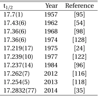
Table 3.4 All published t1/2measurements for19Ne. . . 45
Table 3.5 Parameters used to calculateFt. . . 45
Table 4.1 Technical specifications of BC-501A from[29] . . . 64
Table 6.1 Target thicknesses as measured byαenergy loss in each layer. . . 88
Table 8.1 Measured cross sections for the reaction128Te(3He,n)130Xe at a beam energy of 24.8 MeV. . . 108
Table 8.2 Measured cross sections for the reaction130Te(3He,n)132Xe at a beam energy of 24.8 MeV. . . 113
Table 8.3 Contributions to the systematic uncertainty in the measured cross sections. . . 116
LIST OF FIGURES
Figure 1.1 Feynman diagram forβ−decay. . . 2 Figure 1.2 Mass hierarchy for the neutrinos. The mass difference squared m2
1-m22has been measured but the absolute mass scale is unknown. Additionally, it is un-known whether m3is heavier (normal hierachy) or lighter (inverted hierarchy) than than the other two neutrinos. . . 12 Figure 1.3 Feynman diagrams for 2νββand 0νββdecay[23]. . . 15 Figure 1.4 Simulated spectrum of the summed energy from the two electrons in 2νββand
0νββdecay. For the sake of illustration the 0νββdecay is assumed to have a decay rate 1% of the 2νββdecay rate[23]. . . 15 Figure 1.5 Top panel is the calculated values of the matrix elements for 0νββdecay
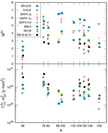
in various candidate isotopes plotted as a function ofA. Bottom panel is the 0νββhalf-life scaled by the effective neutrino mass. The methods and groups making the calculations listed by abbreviation in the legend are non-relativistic and non-relativistic energy density functional theory (NR-EDF and R-EDF), quasi-random phase approximation performed by the Jyväskylä (QRPA Jy), Tübingen (QRPA Tu) and Chapel Hill (QRPA CH) groups, the inter-acting boson model (IBM-2) and shell model calculations performed by the Michigan group (SM-Mi) and the Strasbourg-Madrid and Tokyo groups (SM St-M,Tk). Figure from[58]. . . 17 Figure 1.6 Difference between valence nucleon occupancies in 76Ge and 76Se. Also
shown are the QRPA calculations of the occupancies before and after ad-justing single particle energies to better conform with the experimentally observed values[60]. . . 20
Figure 2.1 Schematic of the 1994 Princeton19Neβasymmetry experiment. Figure from
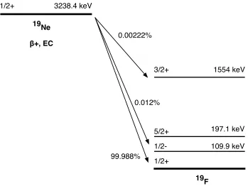
[77]. . . 24 Figure 2.2 Decay scheme for19Ne. . . 28 Figure 2.3 Comparison of the19Neβenergy spectrum from the experiment to the
spec-trum from the simulation. . . 29 Figure 2.4 Residuals in comparison of theβenergy spectrum from the experiment to
the spectrum from the simulation. Over the 550-1900 keV analysis window the two spectra agree to within 0.9%. . . 30 Figure 2.5 Energy walk curve with parameters determined by the fit plotted with60Co
data. . . 31 Figure 2.6 Timing spectrum from the data and the best fit timing spectrum from the
simulation. . . 32 Figure 2.7 The simulated timing spectrum for a single detector over the full range of the
parameter space. The 95% confidence interval is shown in red and the best fit spectrum is shown in blue. In black is the experimental timing spectrum summed from both detectors. . . 32
Figure 3.2 Measured count rate as a function of spin selection slit position[77]. The
dashed lines show the slit positions used during data collection. . . 38
Figure 3.3 Monte Carlo correction as a function of energy. . . 43
Figure 3.4 Experimental data with applied correction from simulation. The value of A0 is extracted from fit with only statistical error quoted. . . 44
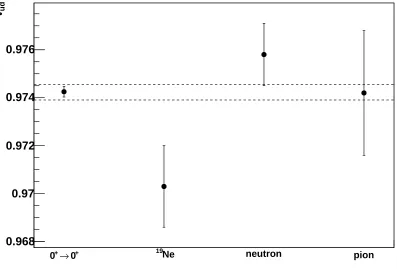
Figure 3.5 Comparison of different determinations ofVu d. The dashed lines represent the average uncertainty of the extracted values ofVu d. . . 46
Figure 3.6 Histogram of contributions to the uncertainty in Vu d. . . 47
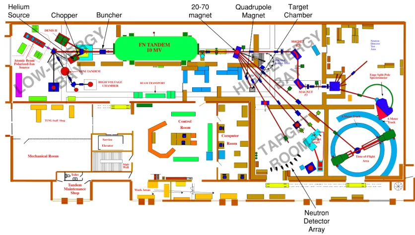
Figure 4.1 Layout of the TUNL tandem accelerator laboratory. Key components of the two proton transfer experiment are labeled. . . 49
Figure 4.2 Schematic of the Helium Ion Source. . . 53
Figure 4.3 Schematic of the duoplasmatron. . . 54
Figure 4.4 Illustration of how the buncher decelerates ions in the head of the pulse and accelerates ions in the tail of the pulse using a properly phased sine wave. Note that the ions in the beam are negative, so the direction of the electric field that accelerates the beam is antiparallel to the direction of travel. . . 57
Figure 4.5 Overhead view of the 70◦beamline. Photo courtesy of David Ticehurst. . . 60
Figure 4.6 Typical signal from capacitive pickoff unit. . . 61
Figure 4.7 Target chamber and interior components. . . 62
Figure 4.8 Drawing of scintillator cell and photomultiplier tube. All dimensions are in inches. Adapted from[50]. . . 65
Figure 4.9 Liquid scintillator detectors cover the range of angles from 0◦ to 18◦ in 3◦ increments. Each angle is covered by three detectors to increase the solid angle and count rate. The middle detector at each angle is level with the ion beam. . . 66
Figure 4.10 Surface barrier detectors arranged as a∆E-E telescope inside the target cham-ber allows for identification of charged particles scattering from the target. . . 67
Figure 4.11 Simplified block diagram of data collection system. . . 69
Figure 5.1 Schematic diagram of the3He recirculation system. The shaded components are the original source parts. . . 72
Figure 5.2 RGA scans taken at the source chamber with no gas flow (background), im-mediately after the start of gas flow (t=0) and after 8 hours of recirculation. . . 74
Figure 5.3 RGA scan taken while cooling oil was leaking into the chamber. Hydrocarbon contamination is noted by the peaks at mass 12 (C), 16 (C H4), 26 (C2H2), 40 (C3H4) and 41 (C3H5). . . 76
Figure 6.1 Target ring dimensions. Adapted from mechanical drawings created by D. Ticehurst. . . 80
Figure 6.3 Drawing of the target holder. Dimensions show distance from center of holder to the edge of a hole and the diameter of each hole. The center of the holder was aligned with the evaporation source and only the four innermost holes were used for target production. Three were used to hold targets and the fourth was reserved for the thickness monitor. . . 84 Figure 6.4 Top plot displays the amount of material needed to create a 2 mg/cm2thick
target as a function of the distance from the source. The bottom plot is the fractional deviation in target thickness across a 1 cm wide substrate as a function of distance from the source. Both plots use the same scale on the x-axis. . . 86 Figure 6.5 An enclosed evaporation boat source holds enriched Te powder during the
deposition of target material onto the substrates. . . 87
Figure 7.1 Comparison of the calculated efficiencies from the PTB code and the KSU code from 7 MeV to 20 MeV. . . 91 Figure 7.2 The deuterium gas cell used in the2H(d,n)3He reaction. Figure adapted from
[105]. . . 95 Figure 7.3 Neutron time of flight spectra from the the2H(d,n) reaction at neutron
ener-gies of 10, 12, 14 and 16 MeV. . . 96 Figure 7.4 Neutron time of flight spectra from the the3H(d,n) reaction at a neutron
energy of 30 MeV. . . 97 Figure 7.5 Detector efficiency as a function of neutron energy. Results from2H(d,n) and
3H(d,n) data compared with simulation. . . 98 Figure 7.6 Relative efficiencies of all 21 neutron detectors. The red line indicates the
mean value and the dashed lines indicate the standard deviation. . . 100
Figure 8.1 (a) Calibration spectrum for TDC generated by pulser. (b) Fit to determine time calibration of TDC channels. The calibration yields 0.1802 ns per TDC channel. The statistical error bars are smaller than the points on the graph. . 104 Figure 8.2 Pulse height plotted against pulse shape discrimination parameter. The dashed
lines represent cuts applied to the data (see text for details). . . 106 Figure 8.3 Energy levels and spin parity assignments in130Xe. . . 109 Figure 8.4 Neutron time of flight spectrum from the liquid scintillator detectors at lab
angle 0◦for the128Te(3He, n) reaction for incident beam energy of 24.8 MeV. Peaks due to transitions to the ground state and excited state are visible. Fits to the data are shown (see text for details). . . 110 Figure 8.5 Differential cross section in center of mass frame of the128Te(3He,n)130Xe
Figure 8.7 Neutron time of flight spectrum from the liquid scintillator detectors at lab angle 0◦for the130Te(3He, n) reaction for incident beam energy of 24.8 MeV. Peaks due to transitions to the ground state and excited state are visible. Fits
to the data are shown (see text for details). . . 113
Figure 8.8 Differential cross section in center of mass frame of the130Te(3He,n)132Xe reaction plotted against the detector angle in the center of mass frame. Data for the ground state and first two 0+excited states are shown. . . 114
Figure B.1 Diagram of the signal from the capacitive beam pickoff. . . 137
Figure B.2 Diagram of the electronics for the silicon surface barrier detectors. . . 138
Figure B.3 Diagram of the electronics used to create the DAQ trigger signal. . . 139
CHAPTER
1
Theory
In this chapter the theory of the weak interaction is briefly reviewed. Single and double beta decay
are discussed in order to provide motivation for the two projects described in this dissertation. The
first of which is the analysis of a precise measurement of the beta decay asymmetry in19Ne. The correlation between nuclear polarization and beta momentum of the isotope19Ne together with the measured lifetime and the decay rate of the muon can be used to extract theVu delement of the
quark mixing matrix. Precise calculations of the elements of the quark mixing matrix are critical in
determing whether the matrix is unitary and to test for physics beyond the standard model. The
second project described in this thesis is a nuclear structure measurement relevant to the calculation
of the matrix element for neutrinoless double beta decay. Double beta decay experiments have
the potential to shed light on the absolute mass scale of neutrinos, whether or not neutrinos are
Majorana particles and finally, whether the neutrino mass hierarchy is normal or inverted. The
precsion of the neutrino mass extracted from a neutrinoless double beta decay measurement, if
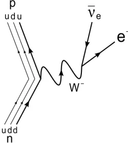
Figure 1.1Feynman diagram forβ−decay.
1.1
Beta Decay
1.1.1 V-A Theory
At the quark level, the decay of the neutron is the transformation of a down quark into an up quark
with the release of an electron and an electron anti-neutrino. Figure 1.1 shows the Feynman diagram
for theβdecay of the neutron. Equation 1.1 describes the amplitude for the reaction assuming the
momentum transfer is much smaller than the mass of the W boson, as is the case forβ decay. In
these equationsGF is the Fermi coupling constant,γµandγ5are the Dirac gamma matrices and
the subscripted variablesψrepresent fermion spinors for the incoming and outgoing particles. The
maximally parity-violating, vector minus axial-vector (V-A) form is apparent in both currents.
M=GpF
2J
µ
l Jµ,h (1.1)
Jlµ=ψνγµ(1−γ5)ψe (1.2)
In moving from an interaction involving bare quarks to one involving nucleons, the leptonic
current remains unchanged but, the hadronic part of the interaction is modified by the strong
force. Equation 1.5 shows the most general Lorentz invariant form for the hadronic current in the
semileptonic decay of a baryon, constructed from the Dirac gamma matrices and the momentum
transferk=kf −ki [48]. The spinors of the initial and final baryon states are denoted byψB and
ψB0,σµνis a second rank tensor constructed from the gamma matrices and thefi andgiare form factors that are functions of the Lorentz scalark2.
Jhµ=Vµ−Aµ (1.4)
Jhµ=ψB0[f1(k2)γµ+i f2(k2)σµνkν+f3(k2)kµ
−g1(k2)γµγ5−i g2(k2)σµνkνγ5−g3(k2)kµγ5]ψB
(1.5)
The conserved vector current (CVC) hypothesis requires that∂µVµis zero. The parameterf3must be zero to satisfy this requirement. In addition, CVC theory equates the form factors in weak decay with
their counterparts in the electromagnetic interaction. As a consequence, the termsf1andf2can be determined by analogy with the corresponding electromagnetic transition matrix elements. In the
non-relativistic limit,f1=1. The paramaterf2is determined by the isovector magnetic moment, which is precisely specified by the magnetic moments of the baryons B and B’ and is often referred
to as the "weak magnetism" form factor.
The use of the G-parity transformation can be used to further classify the parameters. This
operator (equation 1.6) is composed of a 180◦rotation about the second axis in the isospin basis
followed by charge conjugation. Terms that transform with the opposite sign under parity and
G-parity are known as "first class" and terms that have the same sign are known as "second class".
Given that the strong force is invariant under G-parity, the standard model excludes "second class"
terms. This requirement eliminates the parameterg2.
Table 1.1and their transformations.
Parity G-parity Classification
ψψkµ − − 2nd
ψγµψ − + 1st
ψσµνk
νψ − + 1st
ψγ5ψkµ + − 1st
ψγµγ5ψ + − 1st
ψσµνγ5k
νψ + + 2nd
The partially conserved axial current (PCAC) hypothesis states that the axial current is conserved
in the limit that the mass of the pion,mπapproaches zero. In the case of nuclearβdecay the termg3 is negligible[108]as it is suppressed by a factor ofme/mπ. After applying the above considerations
to equation 1.5 the only remaining paramaters aref1,f2, andg1. The only undetermined parameter isg1. Equation 1.7 gives the standard model expression for the hadronic current in nuclearβdecay, where the vector form factorgV is defined as f1(0), the axial-vector form factorgAis defined asg1(0) and the weak magnetism form factorfM is defined asf2(0).
Jhµ=ψB0[gVγµ+i fMσµνkν−gAγµγ5]ψB (1.7)
1.1.2 AllowedβDecay
The allowed nuclearβdecays are a class of decays in which the electron and neutrino carry no
orbital momentum and there is no change in parity from the initial to the final state. In this caseJ,
the total angular momentum of the nucleus, can only change by the spin of the leptons. With each
lepton having spin 1/2, the total change in angular momentum can only be zero or one.
The allowed decays are further subdivided into Fermi and Gamow-Teller transitions based
on spin selection rules. The selection rule for a Fermi transition is∆J=0. The selection rules for Gamow-Teller transitions are∆J=0, 1 excludingJi=0→Jf =0. The so-called superallowed decays
The quantity defined in equation 1.8 is known as theFt value. The terms in the eqation are the statistical rate functionfV, the lifetimet,δ0R is a radiative correction that depends on the nuclear
chargeZ,δN SV is a nuclear structure dependent radiative correction andδVC is an isospin symmetry breaking correction. TheFt value is expected by CVC to be constant over all superallowed decays. In a recent review[65], Hardy and Towner compute theFt value for 20 superallowed decays. The result is an average value of 3072.27(72) s which is constant to within the experimental uncertainty
for each of the transitions and is compelling evidence for the validity of the CVC hypothesis.
Ft ≡fVt(1+δ0R)(1+δ V N S−δ
V
C) (1.8)
1.1.3 Cabibbo-Kobayashi-Maskawa Matrix
The mixing between the first two generations of quarks was first proposed by Cabibbo[38]and
was later extended to three generations by Kobayashi and Maskawa[81]. The mixing between
quark types can be quantified by using a 3x3 rotation matrix (equation 1.9 ) that describes the
transformation between the mass eigenstates of the quarks and their weak flavor eigenstates. It is
often parameterized using three angles and a charge and parity symmetry (CP) violating phase as
shown in equation 1.10 wheresi j =sin(θi j) and similarlyci j =cos(θi j). The values of the
Cabibbo-Kobayashi-Maskawa (CKM) matrix determined by experimental observation are shown in equation
1.12[94].
d0 s0 b0 =
Vu d Vu s Vu b Vc d Vc s Vc b Vt d Vt s Vt b
d s b (1.9)
VC K M=
1 0 0
0 c23 s23 0 −s23 c23
c13 0 s13e−iδ
0 1 0
−s13eiδ 0 c13
c12 s12 0
−s12 c12 0
0 0 1
(1.10)
matrix must be unitary. The squares of the elements in any row of a unitary matrix should sum to
one. The elements in the top row of the CKM matrix are known with the greatest precision and thus
give the strictest test of unitarity.
The value of Vu dcomes from the extractedFt value in superallowed nuclearβdecay[65]. The Ft value can be written as shown in equation 1.11 whereK is a fundamental constant,GF is the Fermi coupling constant,Vu d is the element of the CKM matrix,gV is the vector form factor,MF0is the Fermi matrix element in the isospin symmetry limit and∆V
R is a transition independent radiative
correction. The Fermi coupling constant can be determined independently from muon decay[125].
The other quantities are known or can be calculated. The expression for the Fermi matrix element is
MF0=p(I−I3)(I+I3+1), whereI andI3are the total and third component of isospin, respectively and is equal top2 for superallowed transitions. The only unknown quantity isVu d and thus can be
extracted from the averageFt value.
Ft = K
GF2Vu d2 gV|MF0|2(1+∆VR)
(1.11)
The value ofVu sandVu bare determined from kaon decay andBmeson decay, respectively. The
results of the unitarity test for the first row of the CKM matrix are shown in equation 1.13 and are
consistent with a value of one[94].
VC K M =
0.97417(21) 0.2248(6) 0.00409(39)
0.220(5) 0.995(16) 0.0405(15)
0.0082(6) 0.0400(27) 1.009(31)
(1.12)
Vu d2 +Vu s2 +Vu b2 =0.9996(6) (1.13)
1.1.4 Mixed Decays
axial-vector transitions and the Fermi and Gamow-Teller mixing ratioρ. Equation 1.15 gives the
definition forρ.
Ft = K GF2Vu d2
1
gV2|MF0|2(1+∆V
R)[1+ (fA/fV)ρ2]
(1.14)
ρ=gAM 0
G T gVM0
F
(1+∆AR)(1+δN SA −δA C) (1+∆VR)(1+δVN S−δVC)
1/2
≈gAM
0
G T gVM0
F
(1.15)
The observables in a generalizedβdecay experiment of a polarized nucleus are given in equation
1.16, whereF is the Fermi function,Qis the end point energy,pe andpνare the linear momenta of
the electron and neutrino respectively,Jis the nuclear spin vector,Ee is the energy of the electron andEνis the energy of the neutron. In the subsequent equation
dΓ d EedΩedΩν
=F(Z,Ee)Eepe(Q−Ee)2ξ
צ1+ape·pν EeEν
me Ee +
AJ·pe Ee +
BJ·pν Eν +D
J·(pe×pν)
EeEν ©
(1.16)
ξ=gV2|MF|2+gA2|MG T|2 (1.17)
Integrating over the neutrino variables and neglecting the couplingsb and D which don’t contribute in the standard model gives equation 1.18, whereθis the angle betweenpe andJ.
dΓ
dE dcosθ ∝1+A(E)βcosθ (1.18)
With the mixing parameter and the lifetime, the value ofVu d can be obtained from allowed
decays. Theβ nuclear spin correlationA(E)can be written in terms of the form factors and matrix elements (equations 1.21, 1.22 and 1.23)[71]. In these equationsa=gV|MF| ≈1 is the vector form
factor,b=fM the weak magnetism form factor,
µ= (µ−µ0)/(I3−I30) (1.20)
whereµandµ0represent the magnetic moment of the parent and daughter nuclei andI3andI0 3 represent the third component of isospin for the parent and daughter nuclei,c =gA|MG T|is the axial-vector form factor,W is the total relativistic energy of theβ,W0is the endpoint energy andM is the average mass of the parent and daughter nuclei.
A(E) =f4(E)/f1(E) (1.21)
f1(E) =a2+c2−2E0
3M(c
2+c b) + 2E 3M(3a
2+5c2+2c b)− 2m 2
e
3E M(c
2+c b) (1.22)
f4(E) =−
J
J +1
1/2
2a c−2E0
3M(a c+a b) +
2E
3M(7a c+a b)
+
1
J+1
c2−2E0
3M(c
2+c b) + E 3M(11c
2+5c b)
(1.23)
1.1.5 19Ne Decay
Theβdecay of19Ne is a 1/2→1/2 decay, which means it has both Fermi and Gamow-Teller contri-butions. As such, two experimental observables from the decay are necessary to extractVu d. It is
typical to use the half-life and one of the correlation coefficients in order to determineVu d. Recent
experiments have substantially reduced the average uncertainties in the lifetime of19Ne[34, 116, 118]. However, there is only a single published measurement[40]of the asymmetry. This thesis
de-scribes a new analysis of theβasymmetry measurement of19Ne performed at Princeton University in 1994. This experiment is the most precise measurement to date of the beta asymmetry in19Ne. With a different set of experimental uncertainties and theoretical inputs, a determination ofVu d
uncertainties and provides an important cross check of the nuclear structure-based corrections,
δVN S applied to the superallowed decays.
1.2
Massive Neutrinos
1.2.1 Neutrino Oscillation
The Homestake experiment was designed to measure the solar neutrino flux by detecting the inverse
βdecay reaction on37Cl. It was located 1478 m below ground at the Homestake mine in Lead, SD.
The first results published in 1968 found an electron neutrino flux that was approximately 1/3 the
value predicted by the models of the solar process[47]. Subsequent measurements by the SAGE
collaboration in Russia[3], the GALLEX experiment in Italy[14]and the Kamiokande experiment in
Japan[69]also found a deficit in the number of detected neutrinos relative to prediction.
Results from the Sudbury Neutrino Observatory (SNO) solved the so-called "solar neutrino
problem" and showed direct evidence of neutrino oscillation. The experiment used one kiloton of
pure heavy water (D2O) acting as a Cherenkov detector to measure the solar neutrino flux[32]. The experiment was located 2092 m below the surface or 6010 meters of water equivalent (mwe) at the
Creighton nickel mine near Sudbury, Ontario, Canada. The detector was sensitive to two separate
neutrino induced reactions on deuterons. The first reaction (eq. 1.24) known as the charged current
(CC) reaction is sensitive exclusively to electron neutrinos. The second reaction (eq. 1.25) known as
the neutral current reaction is equally sensitive to all three neutrino flavors. By comparing the rates
of the two reactions, they were able to show conclusively that electron neutrinos originating from
the sun were changing flavor on their way to Earth[7].
νe+d→p+p+e− (1.24)
Table 1.2Measured neutrino paramaters from oscillation experiments. The subscripts indicate values for normal and inverted mass hierarchy. The quantity∆m2is defined as∆m2=m2
3−(m12+m22)/2. Data from
PDG[94].
Parameter Best Fit Value 3σRange
∆m2
21(10−5eV2) 7.37 6.93 - 7.97
|∆m2|(10−3eV2) NH 2.50 2.37 - 2.63
|∆m2|(10−3eV2) IH 2.46 2.33 - 2.60
sin2θ12 0.297 0.250 - 0.354
sin2θ23NH 0.437 0.379 - 0.616
sin2θ23IH 0.569 0.383 - 0.637
sin2θ13NH 0.0214 0.0185 - 0.0246
sin2θ13IH 0.0218 0.0186 - 0.0248
δ/πNH 1.35 0.92 - 1.99
δ/πIH 1.32 0.83 - 1.99
The Pontecorvo-Maki-Nakagawa-Sakata (PMNS) neutrino mixing matrix describes the
trans-formation between the neutrino mass eigenstates and their weak flavor eigenstates. The PMNS
matrix is shown in equation 1.26 where the shorthandci j andsi j is used for cos(θi j)and sin(θi j)
respectively. The matrix is parametrized by the three anglesθ12,θ13andθ23, a CP-violating Dirac
phaseδand two CP-violating Majorana phasesα21andα31.
VP M N S=
c12c13 s12c13 s13e−iδ
−s12c23−c12s23s13eiδ c12c23−s12s23s13eiδ s23c13
s12s23−c12c23s13eiδ −c12c23−s12c23s13eiδ c23c13
1 0 0
0 eiα21/2 0
0 0 eiα31/2
(1.26)
Neutrino oscillation experiments have successfully measured mixing angles and the difference
in neutrino masses, however there are unanswered questions about the neutrino that they are
unable to resolve. A different set of experiments are necessary to determine the absolute scale of
neutrino masses, whether the mass hierarchy is "normal" or "inverted" and whether the neutrino is
a Dirac or Majorana particle.
Neutrino Mass
Normal ?
Inverted m1
m2 m3
m1 m2
m3
Figure 1.2Mass hierarchy for the neutrinos. The mass difference squared m2
1-m22has been measured but
the absolute mass scale is unknown. Additionally, it is unknown whether m3is heavier (normal hierachy)
or lighter (inverted hierarchy) than than the other two neutrinos.
2.05 eV on the mass of the electron neutrino. The KATRIN experiment[55]under construction now,
plans to probe the neutrino mass with an expected sensitivity of 0.2 eV.
1.2.2 Dirac and Majorana Neutrinos
In the standard model, neutrinos are represented by two-component Weyl spinors, as they are treated
as massless and exclusively left-handed. The introduction of neutrino mass implies a coupling
between the left and right-handed chiral fields. One way of giving neutrinos mass is to describe
them as four-component Dirac spinors with left and right-handed components. Ettore Majorana
suggested another method of describing the neutrino in which the left and right-handed chiral
fields are not independent but instead differ by an arbitrary phase, so that they could be described
by a two component spinor[88]. This leads to the Majorana condition shown in eq 1.27 whereC is the charge conjugation operator.
ψR =eiφCψL T
The total fermion field is the sum of its chiral components, as shown in equation 1.28.
ψ=ψR+ψL (1.28)
Combining equations 1.27 and 1.28 it is clear thatψ=CψT which implies that a Majorana fermion is equivalent to its charge conjugate, apart from a possible phase factor. This also implies that a
Majorana fermion is necessarily neutral.
1.3
Double Beta Decay
If the binding energy of the Z+1 nucleus is smaller than the parent nucleus, single beta decay will
not occur but the second order double beta decay could be observed. This process (equation 1.29)
was proposed by Maria Goeppert-Mayer in 1935[63]but was not measured directly until 1987[56].
Since then, double beta decay (2νββ) has been observed in a number of other isotopes. Table 1.3
gives a list of isotopes and the measured values of the double beta decay lifetime for each.
(Z,A)→(Z+2,A) +2e−+2 ¯νe. (1.29)
In 1937, Giulio Racah suggested another mode (equation 1.30) for double beta decay in which
no neutrinos are emitted (0νββ)[97]. It requires that neutrinos are Majorana particles.
(Z,A)→(Z+2,A) +2e−. (1.30)
Outside of one contentious claim of discovery, this process has never been observed[2, 79]. This
decay, if observed, would break conservation of lepton number and would indicate that the neutrino
is its own antiparticle (a Majorana lepton). There are a number of proposed mechanisms underlying
the 0νββdecay. They include the exchange of a heavy neutrino, exchange of supersymmetric (SUSY)
particles as well as exchange of Majorana bosons (also known as majorons)[23]. It has been shown
Table 1.3Measured two neutrino double beta decay half-lifes.
Isotope Half-life (y) Experiment Source 48Ca 6.4+1.4
−1.1×10¹⁹ NEMO-3 [20] 76Ge 1.926±0.094×10²¹ GERDA [6] 82Se 9.6±1.0×10²¹ NEMO-3 [17] 96Zr 2.35±0.21×10¹⁸ NEMO-3 [15] 100Mo 6.93±0.04×10¹⁸ NEMO-3 [15] 116Cd 27.4±1.8×10¹⁸ NEMO-3 [21] 130Te 8.2±0.6×10²⁰ CUORE-0 [10] 136Xe 2.165±0.061×10²¹ EXO-200 [8] 150Nd 9.34+0.66
−0.64×10¹⁸ NEMO-3 [19]
Figure 1.3Feynman diagrams for 2νββand 0νββdecay[23].
are Majorana fermions[102].
If 0νββdecay is moderated by light Majorana neutrinos, then the half-life of the process is related
to the neutrino mass as shown in equation 1.31, where G0νis a phase space factor, M0νis the nuclear matrix element and mββis the effective Majorana mass of the electron neutrino[23]. The expression
for the effective Majorana mass is given in equation 1.32, where the termsUe iin the summation are
the matrix elements in the PMNS neutrino mixing matrix which couple to the electron neutrino.
1
T10/ν2=G
0ν
|M0ν|2|〈mββ〉|2 (1.31)
〈mββ〉=X i
Ue i2mi (1.32)
ββ
FIG. 4 The effective Majorana mass
⟨
m
ββ
⟩
as a function of the mass of the lightest neutrino,
m
lightest
. In making the plot, we have used the best fit values for the parameters in Table I. The
filled areas represent the range possible because of the Majorana phases and are irreducible. If
one incorporates the uncertainties in the mixing parameters, the regions widen. See Bilenky
et al.
(2004) for an example of how the mixing parameter uncertainty affects the regions.
FIG. 5 The distribution of the sum of electron energies for
ββ
(2
ν
) (dotted curve) and
ββ
(0
ν
) (solid
curve). The curves were drawn assuming that Γ
0ν
is 1% of Γ
2ν
and for a 1-
σ
energy resolution of
2%.
Figure 1.4Simulated spectrum of the summed energy from the two electrons in 2νββand 0νββdecay. For the sake of illustration the 0νββdecay is assumed to have a decay rate 1% of the 2νββdecay rate[23].
Additionally, if the 0νββdecay were measured andG0νandM0νwere known then the effective neutrino mass could be determined. The phase space factor can be determined with good precision
[82]. Since the matrix element can only be found experimentally from 0νββdecay, in order to extract
a neutrino mass the matrix element must be calculated. Several methods have been used, but they
disagree with one another by as much as a factor of 3[123]. In the following section the two most
prominent methods will be discussed.
There are a number of experiments proposed and currently underway that are attempting to
find evidence of 0νββdecay. The experimental signature for this decay is a pair of electrons emitted
back to back with summed energy equal to the Q-value of the decay less the negligible amount of
energy going to the recoiling nucleus. If it does occur, the half-life of 0νββdecay is expected to be at
least several orders of magnitude larger than 2νββdecay, given the current limits on the effective
Majorana mass. Given the extreme sensitivity required, the chief concerns for all experimental
searches are the reduction of, or mitigation against background signals near the Q-value of the
Table 1.4Current and proposed neutrinoless double beta decay experiments.
Experiment Isotope Detection Method Source
KamLAND - Zen 136Xe Liquid Scintillator [61]
CUORE 130Te Bolometer [16]
NEMO-3 136Xe Liquid Scintillator [18]
EXO-200 136Xe Liquid TPC [22]
CANDLES 136Xe Liquid Scintillator [119]
GERDA 76Ge Semiconductor [5]
MAJORANA 76Ge Semiconductor [4]
LUMINEU 100Mo Scintillating Bolometer [114]
discuss in detail the techniques employed and challenges faced by the community[23, 57, 68]. Table
1.4 gives a list of experiments searching for 0νββdecay.
1.3.1 Nuclear Matrix Element Calculations
As discussed in the previous section, calculations of the nuclear matrix element for 0νββare
neces-sary to extract the value of the neutrino mass from 0νββdecay lifetimes. This section discusses two
methods for undertaking that calculation as well as their relative strengths and weaknesses.
Sharp discontinuities in the binding energies per nucleon as well as proton and neutron
sep-aration energies give rise to the notion of so called "magic numbers" (Z=2, 8, 20, 50, 86, 128) of
protons and neutrons in nuclei. This is reminiscent of the large discontinuities in ionization energy
indicative of closures in the electronic shells in atomic physics. The nuclear shell model is an attempt
to apply the concept of atomic electron orbitals to nucleons in a nuclei.
The first step in constructing the theory is to establish the potential that the nucleons experience.
A simplistic approach is to use the harmonic oscillator potential. Using this potential is instructive
and yields results that can be determined analytically, however it only correctly predicts the first few
magic numbers. The addition of a term proportional to the square of the orbital angular momentum
levell2flattens the potential at its minima and splits thel degeneracy but still gives essentially the same magic numbers. The solution to the problem of predicting the magic numbers was determined
8
0 1 2 3 4 5 6 7 8M
0 ν SM St-M,Tk SM Mi IBM-2 QRPA CH QRPA Tu QRPA Jy R-EDF NR-EDF 1028 1029 1030 103148 76 82 96 100 116 124 130 136 150
T
1/20
ν
m
ββ
2
[y meV
2
]
A
FIG. 5. Top panel: Nuclear matrix elements (
M
0⌫) for 0
⌫
decay candidates as a function of mass number
A
. All the
plotted results are obtained with the assumption that the
ax-ial coupling constant
g
Ais unquenched and are from di↵erent
nuclear models: the shell model (SM) from the
Strasbourg-Madrid (black circles) [
111
], Tokyo (black circle in
48Ca) [
112
],
and Michigan (black bars) [
82
] groups; the interacting
bo-son model (IBM-2, green squares) [
107
]; di↵erent versions
of the quasiparticle random-phase approximation (QRPA)
from the T¨
ubingen (red bars) [
113
,
114
], Jyv¨
askyl¨
a (orange
times signs) [
81
], and Chapel Hill (magenta crosses) [
115
]
groups; and energy density functional theory (EDF),
relativis-tic (downside cyan triangles) [
116
,
117
] and non-relativistic
(blue triangles) [
118
]. QRPA error bars result from the use of
two realistic nuclear interactions, while shell model error bars
result from the use of several di↵erent treatments of short
range correlations. Bottom panel: Associated 0
⌫
decay
half-lives, scaled by the square of the unknown parameter
m
.
operator
⌧
, which is equivalent to using an e↵ective
value of the axial coupling constant that multiplies this
operator in place of its “bare” value of
g
A'
1
.
27. This
phenomenological modification is sometimes referred to
A.
Shell Model
The nuclear shell model is a well-established
many-body method, routinely used to describe the properties
of medium-mass and heavy nuclei [
119
,
122
,
123
],
includ-ing candidates for
-decay experiments. The model,
also called the “configuration interaction method”
(par-ticularly in quantum chemistry [
124
,
125
]), is based on
the idea that the nucleons near the Fermi level are the
most important for low-energy nuclear properties, and
that all the correlations between these nucleons are
rele-vant. Thus, instead of solving the Schr¨odinger equation
for the full nuclear interaction in the complete
many-body Hilbert space, one restricts the dynamics to a
lim-ited configuration space (sometimes called the valence
space) containing only a subset of the system’s nucleons.
In the configuration space one uses an e↵ective nuclear
interaction
H
e↵, defined (ideally) so that the observables
of the full-space calculation are reproduced, e.g.
H
|
ii
=
E
i|
ii !
H
e↵|
¯
ii
=
E
i|
¯
ii
.
(17)
The states
|
ii
and
|
¯
ii
are defined in the full space and
the configuration space, respectively, and have associated
energy
E
i.
The configuration space usually comprises only a
rela-tively small number of “active” nucleons outside a core of
nucleons that are frozen in the lowest-energy orbitals and
not included in the calculation. The active nucleons can
occupy only a limited set of single-particle levels around
the Fermi surface. Many-body states are linear
combi-nations of orthogonal Slater determinants
|
ii
(usually
from a harmonic-oscillator basis) for nucleons in those
single-particle states,
|
¯
ii
=
X
j
c
ij|
ji
,
(18)
with the
c
ijdetermined by exact diagonalization of
H
e↵.
The shell model describes ground-state nuclear
proper-ties such as masses, separation energies, and charge radii
quite well. It also does a good job with low-lying
excita-tion spectra and with electromagnetic moments and
tran-sitions [
119
,
122
,
123
]. The wide variety of successes over
a broad range of isotopes reflects the shell model’s ability
to capture both the excitation of a single particle from
an orbital below the Fermi surface to one above, in the
spirit of the original naive shell model [
126
,
127
], and
col-lective correlations that come from the coherent motion
of many nucleons in the configuration space. The exact
diagonalization of
H
e↵means that the shell model states
|
¯
ii
contain all correlations (isovector and isoscalar
pair-ing, quadrupole collectivity, etc.) that can be induced by
H
e↵.
This careful treatment of correlations, on the other
Figure 1.5Top panel is the calculated values of the matrix elements for 0νββdecay in various candidateisotopes plotted as a function ofA. Bottom panel is the 0νββhalf-life scaled by the effective neutrino mass. The methods and groups making the calculations listed by abbreviation in the legend are non-relativistic and non-relativistic energy density functional theory (NR-EDF and R-EDF), quasi-random phase approximation performed by the Jyväskylä (QRPA Jy), Tübingen (QRPA Tu) and Chapel Hill (QRPA CH) groups, the interacting boson model (IBM-2) and shell model calculations performed by the Michigan group (SM-Mi) and the Strasbourg-Madrid and Tokyo groups (SM St-M,Tk). Figure from[58].
Suess in Germany[66]. Their contribution was the inclusion of a term coupling nucleon spin to
orbital angular momentum.
The nuclear shell model can be used to calculate the nuclear matrix element for 0νββdecay,M0ν. Most calculations begin with the closure approximation whereM0ν=<f|O|i>and the operator
Ois assumed to be a two-body operator that annihilates two neutrons in the initial nucleus and creates two protons in the daughter nucleus, reducing the implicit sum over intermediate states
to an average value[123]. The next step is to determine the mean field felt by the nucleons. A full
set of single particle states are determined from the potential. States far above the Fermi surface
are assumed to remain unoccupied and not participate in the decay. Similarly, low lying states are
assumed to remain closed and inert. Typically, only a few valence states (five or fewer) are used
in the calculation. Even with a very small number of states, the dimensions of the space becomes
quite large (of order 1010)[45], making the problem computationally intensive. The final piece is the effective interaction which is typically performed using the G-matrix formalism[70]with matrix
elements determined by fits to experimental observables.
Another method for calculating the nuclear matrix element of 0νββdecay uses the quasiparticle
random phase approximation (QRPA) formalism. QRPA assumes the initial and final ground state
nuclei can be treated as a quasiparticle phonon vacuum, analagous to the Bardeen Cooper Schrieffer
(BCS) theory that describes electron pairing in superconductors[25, 113]. Neutron-neutron pairing
and proton-proton pairing are treated separately from neutron-proton pairing. A scaling factorgp p
is often introduced to the neutron-proton pairing strength and is adjusted to reproduce the correct
2νββdecay rate[100, 112].
These two methods for calculating the 0νββnuclear matrix element are complementary. The
strength of the shell model is that it can include arbitrarily complex nucleon correlations.
Unfortu-nately, this power comes at the cost of a Hilbert space that grows rapidly with the number of single
particle states. Despite its limitations, it was used to successfully predict the 2νββhalf-life of48Ca
[44]. The main advantage QRPA has over the shell model is the larger number of single particle
21 single particle states), however the drawback is that QRPA uses simplified nucleon correlations
relative to what can be included in the shell model.
1.3.2 Motivation for Transfer Reactions
Experimental results from nuclear reaction measurements are used by the theoretical community
to serve as a consistency check on calculations. A series of single nucleon transfer reactions were
undertaken in an effort to measure proton and neutron occupancies in76Ge and76Se[78, 103]. Calculations of the occupancies performed using QRPA before the experimental campaign was
undertaken were found to be in poor agreement with the observed occupancies as shown in figure
1.6. After adjusting the single particle energies to conform to the measured occupancy values,
the nuclear matrix element for the 0νββdecay of76Ge was recalculated and found to be in better agreement with shell model calculations[111], indicating the impact of these sorts of measurements.
The BCS description of the ground states of the parent and daughter nuclei at the heart of QRPA
based calculations of the nuclear matrix element of the 0νββdecay can be tested by pair transfer
reactions such as (3He,n) and (t,p). A simple quantitative analysis of the pair transfer reaction indicate that if the BCS condition is true, then transitions to the ground state should experience an
enhancement ofA/4 relative to any 0+excited states[33, 60]. The work of Alford et al. showed that for the tellurium isotopes the strength of the 0+excited states resulting from the (3He,n) reaction was nearly 40% of the ground state[11], indicating a clear departure from the BCS condition.
This dissertation describes a measurement of the proton pair drop off reaction (3He,n) on128Te and130Te performed at the Triangle Universities Nuclear Laboratory (TUNL) on the campus of Duke University. As this reaction has been measured before, the goals of this experiment were twofold. The
first goal was to improve on the previous measurement. That experiment had considerable
system-atic uncertainty due largely to uncertainty in detector efficiency and target thickness. The second
goal of this experiment was to act as a check on a concurrent measurement of74,76Ge(3He,n)76,78Se which was using the same apparatus. A result consistent with the results of Alford et al. for the
J. Phys. G: Nucl. Part. Phys.39(2012) 124004 S J Freeman and J P Schiffer
0.0
0.5
1.0
1.5
2.0
2.5
3.0
Difference in Occ
u
pancy
before after before after1p
0f
5/20
g
9/2NEUTRONS
P
ROTONS
Experiment
QR
P
A
Experiment
QR
P
A
Orbitals
P
articipatin
g
in the Decay
76
Ge ->
76
Se
Figure 6. The changes in orbital occupancies of valence neutron and proton orbits, determined from our experiments [19, 20] are shown as the broader histograms. Alongside, the narrower histograms show the same quantities obtained in QRPA calculations carried out before and after the experiments were published. The changes are shown as positive for both protons and neutrons, even though the neutron number decreases.
be at higher excitation energy (over 3 MeV for 9
/
2
+) and tend to be fragmented into many
small components. In contrast, for the neutron reactions with 42 or 44 neutrons, these nuclei
are about midway between shells and the neutron-transfer centroids are well below 2 MeV
excitation. The normalization procedure for proton transfer therefore had to be somewhat
different from that followed for neutrons.
The (d,
3He) measurements were done at the RCNP in Osaka with the Grand Raiden
spectrograph [
29
]. At this facility the lowest practical energy was 80 MeV for the deuterons,
which still provides reasonable momentum matching for the orbits of interest. For the (d,
3He)
reaction, the momentum matched well for
ℓ
about 2.5, and still reasonable for 1 and 4, thus
suitable for the transitions to p, f and g orbitals of interest. Assuming a single normalization
for the three
ℓ
transfers, one can normalize the DWBA calculations by requiring that the
occupancies be equal to 4.0 for germanium and 6.0 for selenium, providing a fourfold
redundancy in the normalization. This yielded proton occupancies of 3.8, 4.0, 6.1 and 6.2
for the four targets,
74,76Ge and
76,78Se, indicating consistency at the level of around 0.2
nucleons.
The changes in orbital occupancies during the decay, deduced from our measurements,
are shown in figure
6
. The same changes calculated from QRPA before [
30
] and after [
31
] the
publication of the experimental results are also shown in the figure. It is clear that the prior
calculations did not fit the measurements, but adjusting the assumed single-particle energies
in the QRPA considerably improved the agreement and the calculated decay rate changed by
Figure 1.6Difference between valence nucleon occupancies in76Ge and76Se. Also shown are the QRPA calculations of the occupancies before and after adjusting single particle energies to better conform with the experimentally observed values[60].
CHAPTER
2
19
Ne Decay Simulation
In 1994, an experiment to determine the beta asymmetry in the decay of19Ne was performed at Princeton University[77]. Due to inconsistencies in the simulated and measured spectrum of
scattered positrons, the results were never published. In this work we perform a new simulation
and analysis of that experiment using the Monte Carlo software PENELOPEv2002[26].
2.1
The 1994 Princeton Experiment
The19Ne gas was created using the19F(p,n)19Ne reaction utilizing 12 MeV protons from the Princeton cyclotron. The protons struck a water cooled flowing gas target containing SF6[41]. A liquid nitrogen trap removed the remaining SF6. The gas was then pumped into a recirculation chamber containing a 2.5 cm3copper cold “oven" held at 38-40◦K. A small fraction of the atoms escaped from the “oven" and recirculation chamber through a pair of slits with widths of 25 mil and 50 mil respectively. The
remainder return to the “oven" through the recirculation chamber.
Diffusion Pump Stern-Gerlach Recirculation Diffusion Pump
LN Trap2 12 MeV Protons
SF Tank
6 Magnet Detector #1 Detector #2 o o o o o o o o o o o o o o o o o o o o o o o o o o o o o o o o o o o o o o o o Holding Cell Solenoid Needle Valve Buffer Chamber
Source Chamber A-Magnet Chamber
Figure 2.1Schematic of the 1994 Princeton19Neβasymmetry experiment. Figure from[77].
analyzing magnet splits the atomic beam in two, with each beam having a distinct spin state. The
selection slit was positioned so that only atoms of a single spin state could enter the decay region.
Atoms entered the decay cell through a piece of micro channel plate (MCP) with 10µm diameter
pores and 16µm spacing. The tightly collimated beam passed through the MCP into the decay cell
but the random trajectories of the atoms in the trap are highly unlikely to result in gas leaving the
cell. The MCP in essence acted as a one way valve for19Ne gas. Comparison of event rates with and without the analyzing magnet, suggest a conservative upper limit of 1.5% on the fraction of
depolarized atoms that made it through the selection slit.
The polarized gas then passed through a 35 mil wide entrance slit into a rectangular decay trap
with dimensions 2 cm×2 cm×12 cm constructed of 0.5µm thick mylar. The decay trap sits inside
a 0.675 T magnetic field. As the19Ne decayed, positrons from the decay were detected in a pair of 7.46 cm diameter 0.3 cm thick lithium drifted silicon (Si(Li)) detectors with an active region 6.18 cm
in diameter. The detectors were separated by a distance of 1 m. Each detector was divided into four
segments to reduce capacitance and was biased with -400 V DC.
Data collection was arranged in 8 section cycles with the spin states in the following order
shifts in the backgrounds of the detectors. A total of 38 hours of usable data comprised of
approxi-mately 6 million events were collected. The asymmetry was calculated using a super ratio defined
in equation 2.1 and equation 2.2 where the numeric subscripts denote the detector and the up and
down arrows denote spin state and N are integrated counts in the background-subtracted spectrum
for a particular section of the run cycle.
R=N1↑N2↓ N1↓N2↑
(2.1)
A=1− p
R
1+pR (2.2)
2.2
Simulation Model
The experiment was modeled in the Monte Carlo simulation packagePENELOPE[26]. The simulation
geometry included the glass MCP entrance slit, the mylar holding cell, the Si(Li) detectors, the
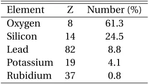
copper coldfinger and the aluminum vacuum enclosure. Table 2.1 gives the atomic composition of
the MCP glass used in the simulation.
Table 2.1Lead glass composition used to model the MCP inPENELOPE.
Element Z Number (%)
Oxygen 8 61.3
Silicon 14 24.5
Lead 82 8.8
Potassium 19 4.1
Rubidium 37 0.8
The z-axis of the model is aligned along the central axis of the solenoid with the origin defined
at the midpoint between the detectors. Equation 2.3 gives an approximation of the central magnetic
for the entire model space is expressed in cylindrical coordinates in terms of an off-axis expansion
of the central (ρ=0) field as shown in equations 2.4 and 2.5[74]. The terms up to fourth order are
used in the simulation.
B0(z) =A1−A2tanh(z+A3)A4 (2.3)
Bz(z,ρ) =
∞
X
n=0 (−1)n∂
2n z B0(z) 22n(n!)2 ρ
2n (2.4)
Bz(z,ρ) = ∞
X
n=0
(−1)n+1 ∂ 2n+1
z B0(z) 22n+1n!(n+1)!ρ
2n+1 (2.5)
Decay events are created with an energy spectrum defined by the Fermi function as shown in
equations 2.6, 2.7 and 2.8, wherepβ is the electron (or positron) momentum,±Z is the number for the final state and is positive forβ−and negative forβ+decay,αis the fine structure constant
andais the nuclear radius divided by Planck’s constant. The simulated energy spectrum and the spectrum from the experiment are shown in figure 2.3 and the fractional deviation is shown in
figure 2.4. Over the 550-1900 keV analysis window the average fractional deviation of the simulated
spectrum relative to the experimental spectrum is 0.9%.
The simulation assumes the decays occur uniformly throughout the interior volume of the
holding cell. The initial direction of the positrons resulting from the decay are distributed
isotropi-cally. The simulation propagates the positrons through the magnetic field using the approximation
method of Bielajew[31]. The basic idea of the method is to track the particles in steps that are
sufficiently small that the acceleration due to the field can reasonably assumed to be constant over
the length of the step. Interactions between the positrons and materials in the model are simulated
inPENELOPEwhich uses the cross sections and angular distributions published by NIST[30].
F =2(1+s)(2pβa)
2s−2eπη|Γ(s+ηi)|2