A Machine Learning Approach to Predict Loan Default.

(1)

ABSTRACT

OWEN, HAILEY MARKAY. A Machine Learning Approach to Predict Loan Default. (Under the direction of Hien Tran.)

In a world of increasing reliance on technology and a culture that wants fast results at the tip of their finger, Lending Club emerges as a fast and mutually beneficial tool to provide borrowers

with unsecured personal loans without the need of interaction with a financial institution and

investors with an opportunity to increase personal wealth by collecting interest on these loans. In this dissertation, we will look at the results given by Decision Tree models, which aim to predict

the time until default on 36 month term loans supplied by Lending Club. First, we will explore loan

default as a binary classification problem. Then, we will expand these results to see how long it will take for a loan to default, using a Multi-Class Decision Tree. We change the question slightly to

determine where in the term of the loan the lender will regain their investment, and whether the

(2)

(3)

A Machine Learning Approach to Predict Loan Default

by

Hailey Markay Owen

A dissertation submitted to the Graduate Faculty of North Carolina State University

in partial fulfillment of the requirements for the Degree of

Doctor of Philosophy

Applied Mathematics

Raleigh, North Carolina

2019

APPROVED BY:

Alen Alexanderian Negash Medhin

Kevin Flores Hien Tran

(4)

DEDICATION

(5)

BIOGRAPHY

Hailey Owen was born 16 June 1989 in Cleveland, Tennessee. She spent her entire childhood in Cleveland through her undergraduate education at Lee University. She began college with a love

of math, but no career direction. She graduated with a B.S. in Mathematics Education and began

looking for a career in teaching. Shortly after graduation, she and her husband, Jared Owen, moved to Princeton, New Jersey where she began to teach grade 5 and 6 mathematics at Princeton Academy

of the Sacred Heart while he completed his graduate degree. After Jared’s graduation, they moved to Raleigh, North Carolina where she enrolled at North Carolina State University in the Applied

Mathematics Ph.D. program. After completing Qualifying exams, she focused her attention on

research in machine learning and predictive analytics.

Still having a heart for education, she accepted an internship in SAS EVAAS in the spring of 2017,

which became a full-time job in spring of 2019. There she is able to use her love of math and passion

(6)

ACKNOWLEDGEMENTS

This journey would not have been possible without the unconditional support I have had from my family, my husband and my parents, who have encouraged me and watched Anderson during my

long days of studying and writing. I owe all my success to you. Anderson, you came into this world

during my second year of study, your existence has pushed me to pursue my dreams so that one day I can help you pursue yours. I love you and you are always my reason.

My friends that have become family, you have all helped in more ways than you know. Some of you offered mathematical help and others offered stress relief. Glenn, I owe you much gratitude for

putting up with my constant doubt and questions. Thank you for your support.

My coworkers at EVAAS, you have made it possible for me to feel successful both professionally and as a student. Thank you for allowing me the time to do it all. I am grateful, and hope to support

you all as you have me.

(7)

BIBLIOGRAPHY . . . 62

APPENDIX . . . 65

(9)

LIST OF TABLES

Table 2.1 Loan Distributions by Loan Purpose . . . 17

Table 2.2 Loan Distributions by Grade . . . 18

Table 2.3 Loan Distributions by Employment length . . . 18

Table 2.4 Class Imbalance Percentages per Model . . . 21

Table 2.5 Error Rates for Sampling Methods . . . 24

Table 2.6 Patterns within Missing Data . . . 25

Table 2.7 Features with Missing Data and Features Most Correlated . . . 28

Table 2.8 Error Rates for Imputation Methods . . . 28

Table 2.9 Features Dropped Before Analysis . . . 29

Table 3.1 Error Rates for Features Engineered . . . 34

Table 3.2 Table of 10 Most Important Features . . . 35

Table 5.1 Error Rates for Classification Tree . . . 50

Table 5.2 Confusion Matrix for Multi-class Classification Tree . . . 50

Table 5.3 Confusion Matrix for Binary Classification Tree . . . 51

Table 5.4 Confusion Matrix for Break-Even Classification Tree . . . 51

Table 5.5 Error Rates for Random Forest Model . . . 55

Table 5.6 Confusion Matrix for Multi-class Random Forest . . . 56

Table 5.7 Confusion Matrix for Binary Random Forest . . . 57

Table 5.8 Performance Metrics for Binary Random Forest . . . 57

Table 5.9 Confusion Matrix for Break Even Random Forest . . . 57

Table 5.10 Performance Metrics for Break-Even Random Forest . . . 57

Table 5.11 Regression Tree Results . . . 58

Table A.1 All Features Used with Description. . . 66

(10)

LIST OF FIGURES

Figure 1.1 An Example of a linearly separable binary problem with support vector ma-chines. Support vector machines build a hyperplane or hyperplanes to classify data. The hyperplane that has the largest distance to the nearest data point of any class is chosen. This maximizes the separation and ideally achieves the lowest error rate[35]. . . 4 Figure 1.2 A decision tree classifier has a root node, which represents the entire

popu-lation or sample of data. This root node gets divided into two or more sets depending on the split and feature that best minimizes the error. This process continues and creates decision nodes until either the node has become pure or a preset threshold has been reached. When splitting stops a leaf or terminal node is created. . . 5 Figure 1.3 k-nearest neighbor algorithm clusters the data to determine similarities. The

model then makes decisions on new data based on labels within each cluster. The cluster size depends on what integer K is determined to be. K is frequently determined by choosing the K that minimizes the error rate[30]. . . 6 Figure 1.4 A neural network makes decisions with layers. Data are passed between

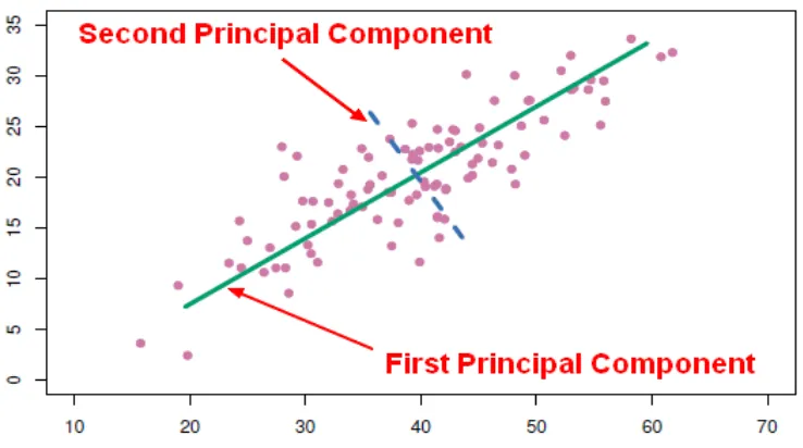
lay-ers to adjust its internal weightings and ultimately minimize classification error. The input layer contains the entire sample or population. There can by many hidden layers depending on how deep the network needs to be achieve accuracy. The output layer contains predictions or decisions made by the model. . . 7 Figure 1.5 The direction with the most variance in the data is represented using the green

line. This is the first principal component. The blue dotted line represents the second principal component and it is the direction that varies the most but is uncorrelated to the first component[9]. . . 8 Figure 1.6 The first principal component is highly correlated with both the features in

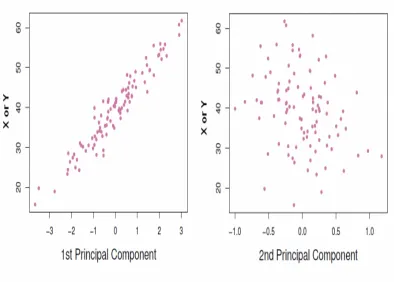
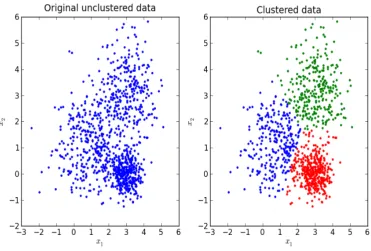
this example. The second has less correlation. As in this example, when the features are highly correlated predictions can be made with one new variable, the first principal component, because it can summarize the data well. Thus the dimension of the data is reduced[9]. . . 9 Figure 1.7 The image on the right was created using the K-Means method for

(11)

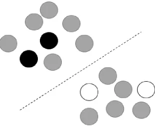
Figure 1.8 An example of a semi-supervised model. The black and white points are labeled while the gray points are unlabeled. From the picture, we can tell that the unlabeled points along with the label points can provide information about the structure of the data that would not be available without the few labeled data points. . . 11 Figure 1.9 Example of Machine Learning Applications[17]for unsupervised, supervised,

and reinforcement learning models. This map shows how each of these types of machine learning might be used in practice. . . 12 Figure 1.10 This is an example of overfitting. The green curve separates the blue and red

data points perfectly. These points are part of the training set. While the error using the green line fore the training set will be zero, the testing set or new data likely will not look the same and result in more error than if the line was more general. This is an example of an over fit classifier. The black line is still separates the training data well, and is far more general. The yellow data point shows the situation where a new data point will be classified differently based on overfitting of the training data. . . 13

Figure 2.1 This figure shows an example of the data used in this project. There are 10 records in this example and a small subset of the features used in each model. 16 Figure 2.2 These two tables show the progression per observation that happens to apply

a one hot encoding. . . 17 Figure 2.3 A map that of the United States from the Census Bureau showing the regions

that were used for recoding of the state variable. . . 19 Figure 2.4 This figure illiterates what is contained in each bin we create for the

multi-class multi-classification tree and random forest model. . . 20 Figure 2.5 The red data points are the minority class in this example, and the green data

points are the majority class[20]. This example was drawn from en example using the well known Iris data set. . . 23 Figure 2.6 This figure shows line segments that are drawn in the feature space between

minority class instances[20]. . . 23 Figure 2.7 This figure shows the synthetic observations the algorithm created. The

al-gorithm randomly chooses one of these line segments to create a synthetic instance. After determining the directions to use, the difference is taken be-tween the instance and its nearest chosen neighbor. That difference is multi-plied by a random number between 0 and 1 and added to the instance. This causes the selection of a random point along the line segment between two specific instances[20]. . . 24

Figure 3.1 Map of United States Showing 3-digit Zip Code Regions . . . 33

Figure 4.1 Basic decision tree structure that defines the root, decision, and leaf nodes. . 37 Figure 4.2 Basic Classification Tree Flow Chart . . . 37 Figure 4.3 This sample of data was used to choose the root note to demonstrate the uses

(12)

Figure 4.4 This figure shows the 3 features that are candidates for the root node along

with the example cut points. . . 40

Figure 4.5 Two Possible Splits to be Made by a Classification Tree . . . 42

Figure 4.6 Confusion Matrix . . . 44

Figure 4.7 Basic Classification Tree Example for Year of Default Selection . . . 46

Figure 4.8 Basic Random Forest, taken from[37] . . . 48

Figure 5.1 Survival Curve by month is created using the survival analysis model. . . 54

Figure 5.2 Actual Survival Plot is based on label instead of prediction. . . 55

(13)

CHAPTER

1

INTRODUCTION

Peer-to-peer lending is the practice of borrowing or lending money from one person or company

to another without going through a bank or other financial institution. Specifically, Lending Club is a peer-to-peer lending platform, headquartered in San Francisco, California[21]. This lending

website pairs borrowers with investors. Customers apply for an unsecured personal loan online.

Borrowers give information about their income, purpose for the loan, and debt. Lending Club collects further information about the borrower such as credit score and credit history then assesses

the risk of funding the loan. If the loan is accepted, Lending Club determines the grade of the loan

which assigns the interest rate and fees that must be paid to Lending Club. Investors can then search through the loan listings to find loans in which they are comfortable with investing based

on information about the borrower, loan amount, grade, and purpose of the loan. Investors make

money by collecting the interest from the loans. Currently, interest rates can range from 5.31% to 26.77% depending entirely on the grade that was assigned to the loan[22]. Investors can choose to

fully fund a loan or partially fund a loan. It is required that investors fund at least $25 in one loan

and invest at least $1,000 in total, but this could be spread over multiple loans. Borrowers can pay back the loan fully at any time without penalty[23].

For borrowers that become delinquent throughout the term of their loan, Lending Club reaches out via email, phone, and letter to collect past due payments and bring the loan back to a â ˘

AIJcurren-tâ ˘A˙I status. After 121 days of failure to pay, a loanâ ˘A ´Zs status is changed to default by Lending Club

(14)

[24]to Lending Club, usually within 150 days of being past due. This could happen sooner if the borrower declares bankruptcy.

Investors have only some details about the loan to make a decision about investing. Knowing

if a person will default and when that could occur could make the decision process less daunting.

In this paper, we will focus on trying to predict the time until charge off. We will do this in several ways. First, we will use a Decision Tree to predict if a loan is charged off, does it happen in the first,

second, or third year of the loan. Second, in an attempt to attain more applicable information to the

investor, we will use a second Decision Tree Model to predict if the loan would be charged off before or after the principal loan amount was paid back to the investor. Finally, we will predict the percent

return on a loan. This is different than all other models run in our research. In this model, we will

use a continuous label and employ a Regression Tree Model. Using this information, lenders, with some certainty, can choose investments that might default, but will be profitable before the loan

goes into default.

1.1

What is Machine Learning?

Dr. Yoshua Bengio, UniversitÃl’ de MontrÃl’al, defines machine learning research as a part of research

on artificial intelligence, seeking to provide knowledge to computers through data, observations and interacting with the world. That acquired knowledge allows computers to correctly generalize to

new settings. Machine learning is based on the idea that systems can learn from data by identifying

patterns within the data. This is done by determining a target function that is an approximation to the relationship between the input data and its label, in the case of supervised learning. This is all

done in hopes that the system will make decisions with minimal human intervention. In general,

machine learning algorithms consist of the following:

• Representation â ˘A¸S Classifiers, i.e. Classification and Regression Trees, Neural Networks, Support Vector Machine, and clustering

• Evaluation â ˘A¸S Accuracy/Error Rate, Confusion Matrix, Information Gain, Sensitivity,

Speci-ficity

• Optimization â ˘A¸S Search Methods, i.e. Gradient descent, Greedy search

Because of recent advancements in methods, research, and computing environments, machine

learning today is not like that of the past. The ability to automatically apply calculations in less and

less time with more and more data has transformed the older idea that machines can learn from patterns within data into what we see today, machines making real time predictions based on real

time data. These advancements have given rise to the applications of machine learning used in

(15)

1.1.1 Supervised vs Unsupervised

There are 3 main ways that classification algorithms operate- supervised, unsupervised, and re-inforcement learning. Supervised learning is done using labeled outputs. The goal of supervised

learning techniques is to learn a function that, given a sample of data and desired (labeled) outputs,

best approximates the relationship between input and outputs that are observable in the data. More explicitly put, the data has a training set that is a complete set with input and labels attached. This

complete data has both features and labels for each observation. The supervised learning algorithm

looks at this complete data to find a pattern. This pattern is used to classify future data either for determining an accuracy measure using the testing set, which also is complete data or classifying

new data that does not have a label. Given a setN of training samples(x1,y1)...(xN,yN)wherexi is a feature vector andy_iis the associated label, it is assumed that there exists a functionf such thaty =f(x)for each of the observes data. The goal of the learning algorithm is to find the best approximationg tof so that it can be applied to new data and assign labels. The functiong is often called a classifier[14].

Machine learning algorithms that use this method are support vector machines, decision trees,

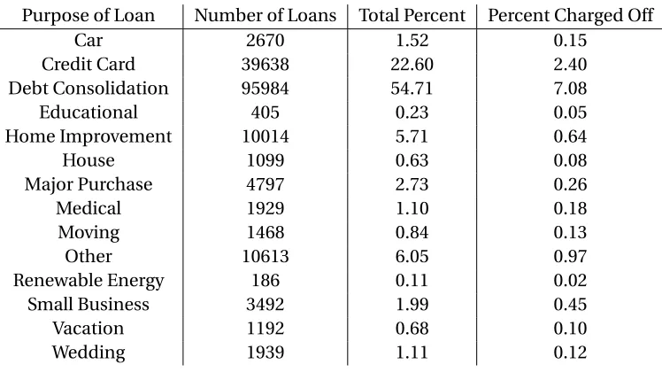
k-nearest neighbor, and neural networks. Support vector machines build a hyperplane or hyperplanes to classify data. This idea can be seen in figure 1.1, whereH₀andH₁are the hyperplanes, and 2

||−→w|| is the distance between the two hyperplanes that is to be maximized to find the optimalH0and

H1. The hyperplane that has the largest distance to the nearest data point of any class is chosen.

This maximizes the separation and ideally achieves the lowest error rate. A decision tree classifier,

which is displayed in figure 1.2, has a root node, which represents the entire population or sample of

data. This root node gets divided into two or more sets depending on the split and feature that best minimizes the error. This process continues and creates decision nodes until either the node has

become pure or a preset threshold has been reached. When splitting stops a leaf or terminal node is

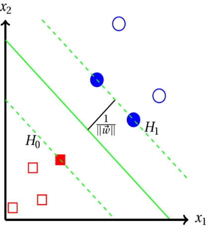
created. This process is explained in great detail in chapter 4. The k-nearest neighbor algorithm clusters the data to determine similarities. It then makes decisions on new data based on labels

within each cluster. In figure 1.3, it can be seen how the algorithm clusters the data. Finally as seen

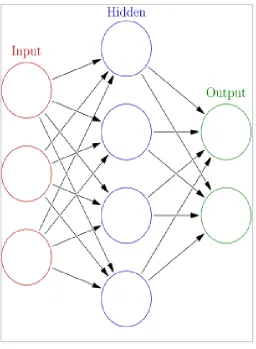
in figure 1.4, a neural network makes decisions with layers. Data are passed between layers to adjust its internal weightings and ultimately minimize classification error.

Unsupervised learning is done with data that does not have labels. The goal is to infer the

natural structure present within a set of data points to make classifications. The two main machine learning algorithms that use this method are principal component and cluster analysis. In principal

component analysis, as illustrated in figure 1.5, the dimension of the data is reduced, but maintains

as much of the complexity of the data as possible. The most significant principal components are selected by looking at how much of the data’s variance they capture, as can be seen in figure 1.6.

(16)

Figure 1.1An Example of a linearly separable binary problem with support vector machines. Support vec-tor machines build a hyperplane or hyperplanes to classify data. The hyperplane that has the largest dis-tance to the nearest data point of any class is chosen. This maximizes the separation and ideally achieves the lowest error rate[35].

the data set’s organization. Cluster analysis is a broad topic that can be accomplished many different ways. Clustering inherently uses the structure of the data to understand how data is similar, as can

be seen in figure 1.7. As explained above, clustering groups data by similarities and then uses those

similarities to gain understating about new data. Assuming the new data is within some distance to existing data, new data can be classified the same way.

Semi-supervised learning allows for some labeled observations in the training set and some

that are not. Due to cost of labeling with some projects, fully labeled data may be near impossible, but some labels can drastically improve results. It can be seen in figure 1.8, that the black and

white points are labeled while the gray points are unlabeled. From the picture, we can tell that the

unlabeled points along with the label points can provide information about the structure of the data that would not be available without the few labeled data points.

Reinforcement learning refers to a goal-oriented algorithm and is used when decisions need to

be made in a sequential order. The input for the model is the initial state from which the model will begin. Each decision is made based on the output of the previous decision. These algorithms are

(17)

Figure 1.2A decision tree classifier has a root node, which represents the entire population or sample of data. This root node gets divided into two or more sets depending on the split and feature that best minimizes the error. This process continues and creates decision nodes until either the node has become pure or a preset threshold has been reached. When splitting stops a leaf or terminal node is created.

of an objective function for reinforcement learning is

Σt=∞ t=0 γ

t_r₍_x₍_t₎_,_a₍_t₎₎_, _(1.1)

wherer is the reward function andt the time or steps it takes to reach the goal.xis the state at

the given time andais the action taken in that state. The objective function calculates all rewards

that could be obtained by running all possible decisions.γt is defined as a discount factor and is multiplied by the reward function. It is designed to make future rewards worth less than immediate

rewards. Reinforcement learning judges decisions that are made by results. The goal is to maximize

the objective function and determine the best path to the goal. An example of a real world application would be a robot who’s goal is to travel from point A to point B. Every inch that the robot moves

closer to its destination could be counted as points thus minimizing the distance the robot travels

from point A to point B.

1.1.2 Applications

Machine learning is used by many industries and has numerous real world applications that have

(18)

Figure 1.3k-nearest neighbor algorithm clusters the data to determine similarities. The model then makes decisions on new data based on labels within each cluster. The cluster size depends on what integer K is determined to be. K is frequently determined by choosing the K that minimizes the error rate[30].

A small number of these applications that deserve mention because how they impact our everyday life

are-• Voice Recognition Software - Virtual Personal Assistants

• Navigation â ˘A¸S GPS

• Advertisement - Product Recommendations

• Face Detection â ˘A¸S Video Surveillance

• Search Engine Results â ˘A¸S Google

• Medical Predictions â ˘A¸S Epidemic Outbreak Prediction

• Fraud Detection - Distinguish between legitimate or illegitimate transactions

Siri and Alexa are popular applications of the virtual personal assistants. These applications use voice commands to find information. Machine learning is an important part of these personal

assistants as they collect information about our lives and preferences and use that information in

(19)

Figure 1.4A neural network makes decisions with layers. Data are passed between layers to adjust its in-ternal weightings and ultimately minimize classification error. The input layer contains the entire sample or population. There can by many hidden layers depending on how deep the network needs to be achieve accuracy. The output layer contains predictions or decisions made by the model.

Networks are employed to allow these virtual assistants to learn how to interpret what the user

wants.

In navigation, recent advancements in machine learning have allowed the GPS to make traffic predictions. While we use the GPS, our current location and velocity, along with many other pieces of

information, are recorded and processed along with thousands of other people to predict traffic and

estimated time until arrival. Many methods discussed above are used in traffic pattern prediction. Fraud detection algorithms are used to distinguish between legitimate and illegitimate

transac-tions. Paypal being one example of a company using machine learning methods to protect against

users laundering money using their services. The company compares millions of transactions using machine learning methods to distinguish between transactions that are considered normal and

(20)

Figure 1.5The direction with the most variance in the data is represented using the green line. This is the first principal component. The blue dotted line represents the second principal component and it is the direction that varies the most but is uncorrelated to the first component[9].

These among so many others are applications of machine learning that are changing the world in

which we are living. In this dissertation, we discuss one other such domain where machine learning

is already making a difference by providing more information to investors about potential loans.

1.1.3 Difficulties in Machine Learning

There are several difficulties that have to be overcome when using machine learning methods. Some

methods have more limitations than others, but it general most machine learning methods struggle when presented with a class imbalance or missing data. Many methods can overfit the data if not

pruned or stopped by defining parameters this can cause models that are too complex and variance

in the results of the model.

Most machine learning algorithms work most efficiently when the number of instances of each

class are roughly equal. When there is a class imbalance, the algorithm typically learns quickly that

the error can be minimized easily by always choosing the larger class. These results are not helpful to the analyst. There are a few ways to overcome this issue and several of them are explored extensively

in this dissertation. Over and under-sampling techniques are used either multiply the minority class

or classes or take away from the majority class or classes. This is usually done by random sampling. Synthetic Minority Over-sampling Technique (SMOTE) is used to create new data by clustering old

(21)

Figure 1.6The first principal component is highly correlated with both the features in this example. The second has less correlation. As in this example, when the features are highly correlated predictions can be made with one new variable, the first principal component, because it can summarize the data well. Thus the dimension of the data is reduced[9].

classes. These methods allow the algorithm to not make decisions based on popularity of one class,

but to minimize the error as they are designed to do.

The problem of having missing data is inevitable when working with real world data. Missing data can be caused by a wide variety of reasons including human error during data entry, humans

withholding information on a survey or form, incorrect sensor readings, or software bugs. There are

also many methods to combat this issue inducing- deletion, mean imputation, clustering methods, and Expectation Maximization. Deleting observations that have missing data is an easy way to avoid

the problem all together if there are minimal missings within the data. This method causes deletion of valuable information if the problem is wide spread and not a good option for those cases. Mean

imputation is a method where each missing data point is filled in with the mean of the feature

it is in. Hot-Deck imputation is a clustering method that is described in detail later in this paper. Expectation maximization is the method that was ultimately chosen as the best method for our data

in this dissertation, and involves an iterative method to find the maximum likelihood estimate for

(22)

Figure 1.7The image on the right was created using the K-Means method for clustering.The goal of the model is to determine groups of data. The number of groups is predetermined by the analyst. To produce these results, first, pick random points as cluster centers, which are called centroids. Second, calculate each inputs distance to each centroid and assign to the nearest. Third, take the average of assigned data points for each cluster and find the new center. Fourth, repeat steps two and three until the center of the clusters no longer change[19].

Overfitting often occurs when the model is more complex than necessary. The algorithm fits the

training data far too closely to generalize results for any new data. It can be seen in figure 1.10, the green curve separates the blue and red data points perfectly. These points are part of the training

set. While the error using the green line for the training set will be zero, the testing set or new data

likely will not look the same and result in more error than if the line was more general. This is an example of an over fit classifier. The black line is still separates the training data well, and is far more

general than a line that fits the data perfectly[16].

1.2

Prior Work

Many methods to predict default in loans have been purposed throughout the literature. Among

(23)

Figure 1.8An example of a semi-supervised model. The black and white points are labeled while the gray points are unlabeled. From the picture, we can tell that the unlabeled points along with the label points can provide information about the structure of the data that would not be available without the few la-beled data points.

[12]. We have chosen to focus our paper on classification and regression tree models and their adaptations. We do this because, while they are generally able to achieve high predictive accuracy

rates, reasoning behind how they reach decisions is interpretable and applicable to both borrowers and lenders[28].

Classification trees were first introduced as methods to classify binary outcomes, but have been used for multi-class problems. In "Solving Multiclass Learning Problems via Error-Correcting Output

Codes"[13], Dietterich et al., generalize the decision tree algorithm to handle multi-class problems.

They take this approach on datasets with 6 classes up to 26 classes.

Much of the previous work has focused on predicting a binary split of loans that will be

paid-in-full or will default. This is done frequently in literature and sometimes as class projects. This is

an easy baseline problem from which to start. One paper that successfully makes this prediction is "Analysis of Default in Peer to Peer Lending"[33]. In this paper, Ramirez explores loan default as a

binary classification problem. He builds a decision tree classifier and evaluates performance based

(24)

Figure 1.9Example of Machine Learning Applications[17]for unsupervised, supervised, and reinforce-ment learning models. This map shows how each of these types of machine learning might be used in practice.

In "A Data-Driven Approach to Predict Default Risk of Loan for Online Peer-to-Peer (P2P)

Lend-ing"[18],the authors use Lending Club data and several multi-class models to predict if a loan will

default, need attention, or be paid and compare results. Their classification/prediction models include neural networks, decision trees, and support vector machines (SVM). They compare the

accuracy of these methods to conclude that SVM achieved the best performance, but only slightly.

This prediction is similar to our baseline prediction though it does use the idea of a multi-class classifier to make a more robust prediction. The novelty of this paper is predicting default times

using classification trees, but until now much of this work was being done using survival analysis.

Narain[29]was the first author to use parametric accelerated failure time (AFT) survival method. He used data that contained 1242 borrowers with 24 month loan terms. He obtained results that

(25)

Figure 1.10This is an example of overfitting. The green curve separates the blue and red data points per-fectly. These points are part of the training set. While the error using the green line fore the training set will be zero, the testing set or new data likely will not look the same and result in more error than if the line was more general. This is an example of an over fit classifier. The black line is still separates the training data well, and is far more general. The yellow data point shows the situation where a new data point will be classified differently based on overfitting of the training data.

their predictions. In "Not if but when will borrowers default", Banasik et al.[3]purposed using an

alternative to the AFT model. His work focused on using the Cox proportional hazard model for its flexible non-parametric baseline hazard. His work used a data set with 50,000 loan applications.

The data was analyzed using the non-parametric proportional hazards model (no baseline hazard

assumption), two parametric proportional hazards models using exponential hazards and Weibull baseline hazards, and an ordinary logistic regression approach[2].

The successes that were found in previous work, using decision trees in creative ways, set the

(26)

1.3

Overview of Contributions

While cleaning the data, imputation, and feature engineering are not novel, the way in which we

employ these methods gives us the ability to apply models to data in a novel way. In literature, we

find countless papers and projects that do a binary decision tree on loan data to determine if a loan will default or be paid-in-full. The accuracy of our models are better than most found in the

literature. These comparisons will be made in chapter 5. The uniqueness in this dissertation comes

in using multi-class classification trees to predict time until default. In the field, similar predictions are made using survival analysis. We compare our results to a survival analysis model in chapter 5.

We finally predict percent gain using a regression tree. We have found in the literature this being

(27)

CHAPTER

2

DATA PREPARATION METHODS

Data cleaning is comprised of detecting and modifying or deleting inaccurate, incomplete, or

irrelevant records or features from a data set. Lending Club’s data had many irregularities and missing values as most of the features are self-reported and some information is not mandatory

on the application. Also, because these data sets come from different years, regulations change

which results in differing or missing entries and inconsistent features. Some, but not all, of these barriers were overcome within the cleaning and preparation process. Another reason for cleaning

and managing the data is to fit the input for the model in the most efficient way possible. Some

features were recoded to reduce computing time.

2.1

Cleaning

The data from Lending Club is publicly available and comes in .csv format in multiple tables. Years 2007-2011, 2012-2013 and the data dictionary were downloaded for this research. After combining

all data sets there was a total of 123,386 loans. A sample of data can be seen in figure 2.1. We wanted

to keep all data where the loan had either been paid-in-full or defaulted. We read in and cleaned this data using SAS 9.4. Initially, we read in and set these tables together to create one large database.

After investigation, we dropped all 60 month term loans. The volume of these longer terms loans is

(28)

qualifications for analysis, thus providing very little data for analysis. After dropping all 60-month

term loans, approximately 11% of loans were default and 89% were paid-in-full. We then found all the features where at least 50% of entries were missing and dropped those out of the study. We also

removed 23 features that had only 31% of their entries missing, but this occurred in the same 54,084

records. The pattern here was too much to meaningfully impute this data. We also removed rows that did not appear accurate, such as if the loan amount was missing. We then found all features

that were created after origination of the loan as these features were not helpful in our research and

dropped those as well. You can see in Table 2.9 the features that were dropped and the reason. All features not mentioned in the table were used in analysis or used to create a feature used in analysis.

Figure 2.1This figure shows an example of the data used in this project. There are 10 records in this exam-ple and a small subset of the features used in each model.

Several features came in the data sets as categorical. Features that were categorical and had no

sense of order or ranking were coded with a one-hot representation. The one-hot representation

creates a new feature for each category within a current feature. An example of this can be seen in figure 2.2. The category that applies to each record is indicated with a 1 and all others 0. An example

of this, in the data, occurs with the feature purpose. This tells us, in 14 categories, the intent of the

borrower. All 14 categories were made into separate features all consisting of 0’s or 1’s. Each record only has one of these 14 categories flagged as the intended use of the resource. You can see in table

(29)

Figure 2.2These two tables show the progression per observation that happens to apply a one hot encod-ing.

Table 2.1Loan Distributions by Loan Purpose

Purpose of Loan Number of Loans Total Percent Percent Charged Off

Car 2670 1.52 0.15

Credit Card 39638 22.60 2.40

Debt Consolidation 95984 54.71 7.08

Educational 405 0.23 0.05

Home Improvement 10014 5.71 0.64

House 1099 0.63 0.08

Major Purchase 4797 2.73 0.26

Medical 1929 1.10 0.18

Moving 1468 0.84 0.13

Other 10613 6.05 0.97

Renewable Energy 186 0.11 0.02

Small Business 3492 1.99 0.45

Vacation 1192 0.68 0.10

Wedding 1939 1.11 0.12

The one-hot representation creates challenges if the number of categories within a feature is large, such as the state in which a borrow lives. If a feature like state is recoded to a one-hot

representation, running the decision tree model becomes far too time consuming. To combat

(30)

Table 2.2Loan Distributions by Grade

Grade of Loan Number of Loans Total Percent Percent Charged Off

A 37555 21.41 1.21

B 66782 38.07 4.06

C 40937 23.34 3.71

D 23442 13.36 2.73

E 5327 3.04 0.70

F 1124 0.64 0.18

G 259 0.15 0.05

Table 2.3Loan Distributions by Employment length

Current Employment Length Number of Loans Total Percent Percent Charged Off

Less than 1 year 14784 8.43 1.10

1 year 12200 6.95 0.87

2 years 16628 9.48 1.19

3 years 14467 8.25 1.04

4 years 11346 6.47 0.80

5 years 13604 7.75 0.96

6 years 10929 6.23 6.79

7 years 9788 5.58 0.73

8 years 7915 4.51 0.57

9 years 6259 3.57 0.44

10+years 49947 28.47 3.32

Did not answer 7559 4.31 0.79

to the feature region. This was done by grouping states into 9 regions then applying the one-hot

representation to the new feature and dropping the original feature of state. These regions were

determined by the Census Bureau[7]and can be seen in figure 2.3.

Features that were categorical, but had meaning when ranked, such as grade, were made numeric

by giving each category a meaningful numeric entry. You can see in table 2.2 the distribution of records by grade. The grade of your loan directly impacts your interest rate. Grade A borrowers will

have the lowest interest rate. These borrowers have been deemed less risky by Lending Club.

2.2

Label Creation

We created four label features to use in our four different model runs. The first label was the binary

label that represented if the loan was defaulted or paid-in-full. We were given the status of the loan

(31)

Figure 2.3A map that of the United States from the Census Bureau showing the regions that were used for recoding of the state variable.

The second feature indicated which third of the term of the loan the borrower defaulted on

payments, if they defaulted. This means that the borrower either paid the loan in full, defaulted

in the first year of first third of the loan term, second year or second third of the loan term, or the third year or final third of the loan term. We then created this label by taking the date that the loan

was issued and the date of last payment and calculating the amount of time between the two dates

to find the total time that payments were being made on the loan. Because we would expect all loans to be paid off or defaulted approximately one or two months after the loan term, we dropped

all records that far exceeded that time frame. We do not have all the payment history details on

each loan; therefore, we do not know enough to proceed with these records. We can see on the Lending Club website that loans that fall delinquent are often brought back to â ˘AIJcurrentâ ˘A˙I by

arrangement of a new payment plan. This could account for the length of some loan terms being

longer than expected[25]. We then took both the binary label, we created, and the total amount of time that was paid on the loan to decide in which of four bins each record should be placed, one of

the bins being paid-in-full, and the other three splitting the loan term in thirds. This is illustrated in

figure 2.4.

(32)

Figure 2.4This figure illiterates what is contained in each bin we create for the multi-class classification tree and random forest model.

amount of the loan, excluding interest, was paid-in-full. Many records within the data set did have

borrowers that defaulted, but did so after their payments had exceeded the amount of the original

loan. In these instances, the lender still made a profit, or at least received the principal amount from the borrower, even though it was not the principal amount plus interest. To calculate if the loan

was profitable or not, we multiplied the number of months the borrower made payments on the

loan by installment paid each month. Then we subtracted that number from the loan amount. If the number was negative or 0, the loan was labeled 1 indicating the loan was profitable, else it was

labeled 0 indicating the lender lost their investment. Default versus paid-in-full was not considered

when creating this label.

The fourth label was created by considering the percent a lender will get as a return on their

investment. We want to be able to predict, with some certainty, what percent of the principal amount the investor will gain or lose. We calculated this by summing the total received principal and the

total received interest, then subtracting the loan amount. This gave us the amount of money that

the investor received from the borrower over the amount that was lent. This total was then divided by the loan amount to find the percent that the investor either gained or lost on the investment.

2.3

Sampling

Another challenge to over come in our data was a severe class imbalance. Decision tree models create biased trees if there is a dominate class. This will frequently result in always predicting the

majority class. A class imbalance was expected as Lending Club does not want to take on loans

(33)

classifier bias when training because of the simplicity of the technique as well as implementation. We

chose to examine three different methods- Over-Sampling, Under-Sampling, and Synthetic Minority Over-Sampling (SMOTE). Across all models, we can see in table 2.5 that SMOTE and Over-Sampling

out perform Under-Sampling. The severity of the class imbalance forces us, when under sampling,

to have so few records that there are not enough to properly train the model.

Table 2.4Class Imbalance Percentages per Model

Multi-Class Label

Percent of Data in Each Class

Paid-in-full 87.37%

Default Year 1 4.59%

Binary Label

Paid-in-full 87.37%

Default 12.63 %

Break-Even Label

Gain from Investment 88.72%

Loss from Investment 11.28%

2.3.1 Over-Sampling the Minority Class

Over-sampling is done by generating new records that are copies of existing records. This process

must be done after removing the validation set to prevent over fitting. We do not want the same records to be trained on as we will use to validate our models. Our over-sampling was done by first

randomizing the data. We removed testing and validation sets. We then duplicated the minority

class(es) until the percentages in the data were approximately equal to the majority class. We did investigate making the classes exactly equal by randomly selecting records to duplicate instead of

(34)

2.3.2 Under-Sampling the Majority Class

Under-sampling is done by decreasing the number of records in the majority class until it is compa-rable in size to the minority class. This is done by randomly selecting records to keep in the class.

Our under-sampling was done by first randomizing the data a second time. We sampled using a

simple random sampling method. In simple random sampling, each unit has an equal probability of selection, and sampling is without replacement. We drew only the number of records that were in

the majority class. This severely depleted the number of records that were available to our model.

Due to the lack of information given to the model, this method did not create favorable results. If more data were available, this method could be a better option.

2.3.3 SMOTE

SMOTE is a common method of over-sampling. Instead of duplicating records, the algorithm creates records that are synthetic to append to the minority class. Synthetic records are created by looking

along the line segments, in the feature space, between minority class instances. The algorithm

draws a line segment between each instance and its k nearest neighbors, then randomly chooses one of these line segments to create a synthetic instance. After determining the directions to use,

the difference is taken between the instance and its nearest chosen neighbor. That difference is

multiplied by a random number between 0 and 1 and added to the instance. This causes the selection of a random point along the line segment between two specific instances. This idea is depicted in

figures 2.5, 2.6, and 2.7. The algorithm will continue this process until the classes are balanced. This

approach effectively forces the decision region of the minority class to become more general[8]. Our implementation uses five nearest neighbors.

2.3.4 Sampling Results

Imbalance within classes was by far the biggest hurdle in processing the data. The class imbalance was so severe combined with our high dimensional data set, the SMOTE algorithm was unable to

really compete with over-sampling. In a paper by Blagus and Lusa[4], it was concluded that even

though SMOTE performs well on low-dimensional data, it is not effective in the high-dimensional setting for many classification methods, including classification trees. Under-sampling sharply

depleted the amount of data fed into the classifier. The lack of data caused unfavorable results

coming out of the model. It can be seen in table 2.5, over sampling is the superior method. It is also much less complicated and takes far less time to implement.

We are using error rate of our decision tree model to make decisions on methods to use to finalize

(35)

Figure 2.5The red data points are the minority class in this example, and the green data points are the majority class[20]. This example was drawn from en example using the well known Iris data set.

Figure 2.6This figure shows line segments that are drawn in the feature space between minority class instances[20].

to become as small as possible while taking into account the false positive rate as well, which is

(36)

Figure 2.7This figure shows the synthetic observations the algorithm created. The algorithm randomly chooses one of these line segments to create a synthetic instance. After determining the directions to use, the difference is taken between the instance and its nearest chosen neighbor. That difference is multiplied by a random number between 0 and 1 and added to the instance. This causes the selection of a random point along the line segment between two specific instances[20].

Table 2.5Error Rates for Sampling Methods

Multi-Class Label Binary Label Break-Even Label

SMOTE 37.23% 34.58% 33.83%

Over Sampling 23.99% 22.15% 20.49%

Under Sampling 47.48% 45.32% 44.13%

2.4

Imputation

A serious problem when working with real-world data is that there are often significant amount of data missing for various reasons. When working with a limited amount of data, it is crucial to use all

available data and not discard records due to missing values if possible.

Lending Club compiles a large amount of financial and personal data from its borrowers. This data is plagued with missing entries, some explainable and some that are seemingly erroneous. In

section 2.1, we discussed our method of removing features due to having more than 50% missing

from the feature. In the cases where the missing information was seemingly random we elected to attempt two forms of imputation to gain precision. We employed two popular methods- Nearest

Neighbor Hot-deck and Expectation Maximization. We evaluated the performance of each based on

(37)

choosing a â ˘AIJdonorâ ˘A˙I row to use for the missing value, the expectation maximization imputes

missing values by finding the maximum likelihood estimates and iterates until maximizing the log likelihood. Then it uses this estimate to impute the data.

2.4.1 Removing Missing Data

Removing missing data involved deleting records in our data set that are missing data in any feature

of interest. This is a common technique because it is easy to implement and works with any type of analysis. Because we needed a baseline for our imputation attempts, we started this process by

deleting all records with missing data anywhere in them. We deleted 9,036 records.

Table 2.6Patterns within Missing Data

Group 1 2 3 4 5 6 7 8 9 10 11 12

tax_liens X X X X X X X X

total_acc X X X X X X X X X X

collections_12_mth_ex_med X X X X X

acc_now_delinq X X X X X X X X X X

chargeoff_within_12_mths X X X X X

delinq_amnt X X X X X X X X X X

earliest_cr_line X X X X X X X X X X

revol_util X X X X X X

pub_rec_br X X X X X

pub_rec X X X X X X X X X X

open_acc X X X X X X X X X X

delinq_2yrs X X X X X X X X X X

emp_length X X X X X X X X X X

annual_inc X X X X X X X X X X X

inq_last_6mths X X X X X X X X X X

Frequency 166093 7542 1203 143 6 4 32 2 74 1 25 4

As you can see in Table 2.6, groups 11 and 12, most features are missing values in these 29 records

(25 from group 11+4 from group 12). Although it is impossible, by looking at the data, to tell the reason these 29 records are missing values from nearly all 15 features, it might imply there is an

underlying pattern of missingness among these records. Therefore, we dropped these 29 records. This also eliminates the need to impute total_acc, acc_now_delinq, delinq_amnt, earliest_cr_line,

(38)

2.4.2 Expectation Maximization

The Expectation Maximization (EM) Algorithm is a technique that is used to impute missing values by finding the maximum likelihood estimates. This is done by using an iterative process with

two main steps- the expectation step, or E step and the maximization step, or the M step. These

two steps are repeated until convergence. Though the EM algorithm was used earlier for special circumstances, in a paper from 1977, Dempster, Laird, and Rubin[11]generalize and formally

formulate the Expectation Maximization algorithm[1]. To use the EM algorithm in our incomplete

data problem, we must associate it with the complete data problem to estimate the maximum likelihood. The initial step in the algorithm is to initialize the parameter vector, let this beΘ.

Lety denote the complete data samples, withy ∈Y ⊆Rm, and the probability density function (pdf ) that is associated withy beP_y(y;Θ).y, however, cannot be directly observed. We will refer to our observed data asx=g(y)∈Xo b⊆Rl, wherel <m. The pdf associated with the observed data isPx(x;Θ). The subset ofy’s associated with a singlexcan be written asY(x)⊆Y. The pdf of the incomplete data can be found by

Px(x;Θ) =

Z

Y(x)

Py(y;Θ)d y. (2.1)

Ideally, the Maximum Likelihood estimate ofΘ, denoted ˆΘM L, would be given by

Σk∂l n(Py(yk;Θ))

∂Θ =0. (2.2)

Our problem is that they’s represent our complete data, which is not available. Here is where we

use the EM algorithm to combat this issue.

For the current value ofΘ(t), the parameter vector, the E step computes the expected value of the observed data log-likelihood

Q(Θ|Θ(t)) =E[Σkl n(Py(yk;Θ)|X,Θ(t))]. (2.3)

The M step finds the parameter vector that maximizes the log-likelihood of the imputed data. We call this vectorΘ(t+1)_{and our goal is to maximize}_Q_(Θ_;_Θ(t)₎_{. That is}

∂Q(Θ;Θ(t))

∂Θ =0. (2.4)

The initial estimate is begun atΘ(0)and iterations are continued until the following condition is met:

||Θ(t+1)

(39)

Because the log-likelihood increases at each step and is bounded from above, convergence is

guaranteed. Proof of this can be found in[11]on page 7.

2.4.3 Hot-Deck

Hot-deck Imputation is an intuitive method for handling incomplete data. Therefore it has been

used propitiously on large data sets[27]for many years. We employed nearest neighbor hot deck

imputation. In this method, missing values are replaced by values from similar complete samples. These similarities are found by clustering the data. We must define a metric to measure distance

between complete data and data with missing information. Suppose ourX indicates features with

missing data withmmissing values andY indicates complete features.

To choose which value ofXiwherei=1, ...,n−mreplaces the missing inXj where j=n−m+ 1, ...n, we must look at the corresponding values in the complete dataY. By calculating the closest

valueY_j toY_i, we determined which samples were most similar. The distance is calculated using the following method:

|Yi−Yj|= min

1≤k≤n−m|Yk−Yj| (2.6)

If two or more values are equidistant fromYj, the mean of the correspondingXiis calculated for imputation.

We looked to see what features had missing data. This can be seen in Table 2.6. We then analyzed which features were most correlated with the feature containing missing data. The feature most

correlated will beY as in our equations above. You can see in Table 2.7 the features and their

(40)

Table 2.7Features with Missing Data and Features Most Correlated

Feature with Missing Data Feature Most Correlated Correlation Rate

emp_length_num mortgage 0.214

tax_liens_num pub_rec_num 0.643

collections_12_mths_ex_med_num int_rate_num 0.043

chargeoff_within_12_mths_num delinq_2yrs_num 0.114

pub_rec_br_num pub_rec_num 0.753

revol_util_num int_rate_num 0.412

2.4.4 Imputation Results

As we see in Table 2.8, the EM algorithm sightly outperforms both Hot-deck Imputation and simply removing the missing data in every model. In our situation, Expectation Maximization is a good

fit for the type of data we have. Features we imputed had at most 4% of the data missing, and it is

important to us that they preserve the relationship with other features for its use in the decision tree model.

Table 2.8Error Rates for Imputation Methods

Remove Missing Data 23.99% 22.39% 21.26%

EM 23.99% 22.15% 20.49%

Hotdeck Imputation 24.27% 22.15% 20.84%

2.5

Contributions

While creating the labels, sampling, and imputing missing data are not novel, the way in which

we employ these methods gives us the ability to run the model to produce results that are novel. In literature, we find countless papers and projects that do a binary decision tree on loan data to

determine if a loan will default or be paid-in-full. The uniqueness in this dissertation comes in the

(41)

Table 2.9Features Dropped Before Analysis

Feature Dropped Reason

all_util All Missing

acc_open_past_24mths Not collected Prior to 2012

annual_inc_joint All Missing

application_type All entires are the same

avg_cur_bal 31% Missing

bc_open_to_buy Not collected Prior to 2012

bc_util Not collected Prior to 2012

collection_recovery_fee Data recorded into the life of the loan

deferral_term All Missing

dti_joint All Missing

emp_title Can’t be used in analysis

hardship_amount All Missing

hardship_dpd All Missing

hardship_end_date All Missing

hardship_last_payment_amount All Missing

hardship_length All Missing

hardship_loan_status All Missing

hardship_payoff_balance_amount All Missing

hardship_reason All Missing

hardship_start_date All Missing

hardship_status All Missing

hardship_type All Missing

hardship_flag All enties are the same

id All Missing

il_util All Missing

inq_fi All Missing

inq_last_12m All Missing

last_credit_pull_d Data recorded into the life of the loan last_pymnt_amnt Data recorded into the life of the loan

max_bal_bc All Missing

member_id All Missing

mo_sin_old_il_acct 31% Missing

mo_sin_old_rev_tl_op 31% Missing

(42)

Table 2.9(continued)

mo_sin_rcnt_tl 31% Missing

mort_acc Not collected Prior to 2012

mths_since_last_delinq 58% missing

mths_since_last_major_derog 86% missing

mths_since_last_record 90% missing

mths_since_rcnt_il All Missing

mths_since_recent_bc_dlq 84% Missing

mths_since_recent_inq 31% missing

mths_since_recent_revol_delinq 76% missing

mths_since_recent_bc Not collected Prior to 2012 next_pymnt_d Data recorded into the life of the loan

num_accts_ever_120_pd 31% missing

num_actv_bc_tl 31% missing

num_actv_rev_tl 31% missing

num_bc_tl 31% missing

num_il_tl 31% missing

num_op_rev_tl 31% missing

num_rev_accts 31% missing

num_rev_tl_bal_gt_0 31% missing

num_tl_120dpd_2m 31% missing

num_tl_30dpd 31% missing

num_tl_90g_dpd_24m 31% missing

num_tl_op_past_12m 31% missing

num_bc_sats Not collected Prior to 2012

num_sats Not collected Prior to 2012

open_acc_6m All missing

open_il_12m All Missing

open_rv_12m All Missing

open_rv_24m All Missing

orig_projected_additional_accrue All Missing

out_prncp Data recorded into the life of the loan

(43)

Table 2.9(continued)

payment_plan_start_date Data recorded into the life of the loan

pct_tl_nvr_dlq 31% missing

percent_bc_gt_75 Not collected Prior to 2012

policy_code All entires are the same

pymnt_plan Data collected after origination recoveries Data recorded into the life of the loan

revol_bal_joint All Missing

sec_app_chargeoff_within_12_mths All Missing

sec_app_collections_12_mths_ex_m All Missing

sec_app_earliest_cr_line All Missing

sec_app_inq_last_6mths All Missing

sec_app_mort_acc All Missing

sec_app_mths_since_last_major_de All Missing

sec_app_num_rev_accts All Missing

sec_app_open_acc All Missing

sec_app_open_il_6m All Missing

sec_app_revol_util All Missing

tot_coll_amt 31% missing

tot_cur_bal 31% missing

tot_hi_cred_lim 31% missing

total_bal_il All Missing

total_cu_tl All Missing

total_il_high_credit_limit 31% missing

total_pymnt Data recorded into the life of the loan

total_pymnt_inv Data recorded into the life of the loan total_rec_late_fee Data recorded into the life of the loan

total_rev_hi_lim 31% Missing

total_bal_ex_mort Not collected Prior to 2012 total_bc_limit Not collected Prior to 2012

url All Missing

(44)

CHAPTER

3

FEATURE ENGINEERING

Feature engineering is a process of the analyst creating features by either using relationships among

features currently in the data or looking for outside information that can be merged onto the data with already existing features. Feature engineering is the human element in machine learning.

Understanding of the data, domain knowledge, and human intuition and creativity are what allow

feature engineering to make a difference in model accuracy. Decision Trees are designed to find relationships among features and uses those to achieve better results. In general, a well engineered

feature may be easier for the algorithm to digest and make rules from than the feature from which it

was derived.

In our data, we created one relationship that increases accuracy. First credit pull (first_cr_pull)

is time between earliest credit line and loan origination. This gives the model the amount of time

that a borrower has had at least one credit line open. You can see in table 3.2, first credit pull is of significant importance to all three models that were run.

In our data set, we were provided with the first three digits of a zip code for each borrower. This

allowed us to know what state and what region of the state each borrower was associated with at the time the loan was originated.

We also wanted to get a picture of how far the borrowers income was away from the average income in their general area. The only two location variables we had for each borrower was the

first 3 numbers in the zip code and the state in which they reside. We used a zip code database

(45)

contained income information per capita. We used a data set that provided average income per

county, but did not contain zip code. Both data sets were pulled from the census bureau database. We merged these two data sets by county, and calculated the average income in each 3 digit zip code

region.

To create the relationship for the new feature, percent difference from the average income, we looked at each borrowers income and the average income in their region. We then calculated the

percent difference and the percent increase.

p e r_d i f = ₁ |a v e r a g e_i n c o m e−a n n u a l_i n c o m e|

2×(a v e r a g e_i n c o m e+a n n u a l_i n c o m e)

×100 (3.1)

p e r_i n c r e a s e =a n n u a l_i n c o m e−a v e r a g e_i n c o m e

a n n u a l_i n c o m e ×100 (3.2)

As a result of adding these features, the error rate decreased, as seen in table 3.1. Also, in table 3.2, percent difference in income (per_dif ) was 10th most important in all models run. This tells us

that this feature is useful to the models, and made a difference in its calculations.

(46)

3.1

Feature Engineering Results

Table 3.1Error Rates for Features Engineered

Before Feature Engineering 23.99% 22.15% 20.49%

First Credit Pull 23.54% 21.85% 20.20%

Percent difference in Income 23.48% 21.71% 20.07%

Percent Increase in Income 23.57% 21.83% 20.13%

With all Engineered Features 23.46% 21.63% 19.67%

3.2

Feature Importance

Feature importance is calculated within a decision tree model while it is splitting, which will be

discussed more in chapter 4. The importance score is calculated as the decrease in node impurity weighted by the probability of reaching that node. The probability of reaching a node is calculated

by the number of samples that reach the node, divided by the total number of samples. The higher the importance score the more important the feature is to the model.

In Table 3.2, we can see the top ten most important features in all decision tree models. We notice

that all three models approximately score the same 10 features most important. We are asking each model run to make similar decisions all based on giving a loan to someone based on their financial

characteristics, thus using the same features for each model is not a surprising result. Similarly,

professionals, such as loan officers or investors, use certain criteria for loans, to decide if they are good investments to fund.

3.3

Contributions

Feature engineering is not a unique method in machine learning; however, its creative aspect does lend itself to finding new ways to allow the model to incorporate data. In this way, we calculated

three features that are definitely used in the field, possibly inadvertently, to make decisions about

(47)

Table 3.2Table of 10 Most Important Features

Importance Score Feature

Multi-Class Label

0.078 dti_num

0.078 revol_bal_num

0.075 revol_util_num

0.065 loan_amnt_num

0.064 annual_inc_num

0.053 earliest_cr_line_num

0.053 total_acc_num

0.053 first_cr_pull

0.044 int_rate_num

0.044 per_dif

Binary Label

0.076 dti_num

0.071 revol_bal_num

0.060 New_England

0.056 total_acc_num

0.056 loan_amnt_num

0.049 first_cr_pull

0.046 per_dif

Break-Even Label

0.075 dti_num

0.074 revol_bal_num

0.059 New_England

0.059 loan_amnt_num

0.054 first_cr_pull

0.050 total_acc_num

(48)

CHAPTER

4

METHODS

4.1

Classification Tree

The idea of classification and regression trees was introduced by Breiman et al. in 1984[5]. The basic

goal of a classification tree is to split a population of data into smaller segments. This algorithm has a tree-like structure, hence the name. Each internal node represents features, each branch represents

a rule made by the algorithm, and each leaf the outcome of those decisions. In figure 4.1 we see a basic example of the decision tree structure. A tree uses if-then statements to find patterns in

data. Each of these if-then statements creates the branches. Elements to the left of that point get

categorized in one way, while those to the right are categorized in another. Each non-terminal node, determined by several parameters, repeats the splitting process until a specified level of purity is

reached. Decision trees are grown by examining all possible splits of all input features. The algorithm

then decides if the criterion has been met or not[35]. In figure 4.2, we see a basic flow chart for how a decision tree is created as well as how the data flows though the process of creation. Each piece of

this flow chart is discussed, in detail, throughout this chapter.

There are two stages to prediction. The first is training the model where the tree is built and optimized by using the training and validation sets. The second is predicting where we use the

(49)

Figure 4.1Basic decision tree structure that defines the root, decision, and leaf nodes.

Figure 4.2Basic Classification Tree Flow Chart 4.1.1 Classification Tree Model

(50)

that the samples with the same labels are grouped together.

Let the data at nodembe represented byQ. For each candidate splitΘ= (j,tm)consisting of featurej∈1, ,nand thresholdtm, partition the data intoQl e f t(Θ)andQr i g h t(Θ)subsets where

Ql e f t(Θ) = (x,y)|xj≤tm (4.1)

Q_{r i g h t}(Θ) =Q\Q_{l e f t}(Θ). (4.2) The impurity at the pointmis determined using an impurity functionH(·), for which there are several choices depending on the problem being solved. This is discussed later in the chapter. The total impurity,G(·,·), (weighted by the number of samples in the nodes) is computed using the impurity functionH(·)as follows,

G(Q,Θ) =nl e f t

Nm