ABSTRACT
ZRIDA, MARWEN. A Game-Theoretic Approach for the Optimal Strategies of the Transboundary Pollution Problem with Emission Permit Trading and Banking (Under the direction of Dr. Negash Medhin).
A Game-Theoretic Approach for the Optimal Strategies of the Transboundary Pollution Problem with Emission Permit Trading and Banking
by Marwen Zrida
A thesis submitted to the Graduate Faculty of North Carolina State University
in partial fulfillment of the requirements for the degree of
Master of Science Operations Research Raleigh, North Carolina
2017
APPROVED BY:
_______________________________ _______________________________ Dr. Negash Medhin Dr. Tao Pang
Committee Chair
BIOGRAPHY
ACKNOWLEDGMENTS
I would like to express my deepest gratitude to my advisor and committee chair Dr. Negash Medhin who provided a precious and continuous help throughout my journey in North Carolina State University. Through his assistance, he greatly helped me in the completion of my thesis. I also want to thank my committee members Dr. Tao Pang, Prof. Jeff Scroggs and Prof. Reha Uzsoy for their hard work and dedication as my advisory committee.
I would also like to thank our department Graduate Services Coordinator Linda C. Smith for her assistance with the many administrative details during my time at NCSU.
TABLE OF CONTENT
LIST OF FIGURES…………..………...…...………...v
Introduction to the Transboundary Pollution Problem and Literature Review ... 1
Modeling and Analysis………….……….10
2.1 Assumptions and basic model..………10
2.2 The noncooperation Scenario…....……….…….14
2.3 The cooperation Scenario……..……….…….21
2.4 Comparison between cooperation and non-cooperation outcomes...…...27
2.4.1 Emission level comparison……...………...27
2.4.2 Emission market comparison…….………28
2.4.3 Net revenue comparison………...………...29
Model Refinement ... 31
3.1 Introducing the banking feature……….31
3.2 The optimal strategy...……..………...…….35
Numerical Example ... 44
4.1 The noncooperative scenario….…………..………45
4.2 The cooperative scenario……...………...47
4.3 Comparison…………...……….…...49
4.4 With banking……..…...………...51
Conclusion ... 54
LIST OF FIGURES
Figure 1: Carbon dioxide level profile from the 50's up to now ... 2
Figure 2: The optimal pollution stock evolution with no cooperation... 47
Figure 3: The optimal pollution stock evolution with cooperation... 49
Figure 4: The optimal pollution stock evolution with and without cooperation... 51
CHAPTER 1
Introduction to the Transboundary Pollution Problem and
Literature Review
Pollution and global warming have emerged as one of the most critical issues humanity is facing. According to NASA, 9 of the 10 warmest years recorded have occurred since 2000. Scientists unanimously link this increase in temperatures to the increase in carbon dioxide emissions. As a matter of fact, NASA reports that carbon dioxide levels are at their highest in 800,000 years. According to the National Oceanic and Atmospheric Administration's (NOAA), Earth System Research Lab, the average level of carbon dioxide (CO2) in earth's
atmosphere reached over 400 parts per million for the month of April 2014. Carbon dioxide levels were almost 280 ppm before the industrial revolution, when humans first began emitting large amounts of CO2 into the atmosphere by burning fossil fuels. When Charles David Keeling
Figure 1: Carbon dioxide level profile from the 50's up to now
Increasing amounts of CO2 and other gases is caused by the burning of oil, gas and coal,
by their own population, but the gases emitted by these polluters will not only affect the American, Chinese or European Union citizens. Every single human being and living creature will almost equally suffer from these emissions. Pollution is a particularly controversial issue because it does not obey the laws of borders and territory sovereignty. Emissions released by a country can travel via air or water and affect other countries that are hundreds and sometimes thousands of miles away. This problem is known as the transboundary pollution phenomenon.
The Sandoz spill that occurred in November of 1986 in Basel, Switzerland is an example of a transboundary pollution cases affecting several countries. Sandoz is a chemical manufacturing company that experienced an agrochemical warehouse fire that resulted in the release of over 40 tons of toxic chemicals into the Rhine River. In December, it was reported that fish population in the Rhine was completely exterminated, and the River could not be used as a drinking water source for more than two weeks. The spill affected 6 countries in total (Switzerland, Principality of Liechtenstein, Austria, Germany, France and the Netherlands). Switzerland was found responsible for not notifying the affected countries in time so that proper actions could be taken to prevent contamination. The spill led to new legislation regarding spill liability and a new emphasis on communication between the countries including the Rio Declaration, which obliges the member states to instantaneously inform other states of any disaster.
Consolidated Mining and Smelting Company (COMINCO) and has processed lead and zinc since 1896. Damages were caused to forests and crops in Washington State by the release of smoke that crossed the US-Canadian border. The pollution caused by the Canadian company affected the farmers in Washington State who expressed their discomfort and asked for compensation. The matter was transmitted to tribunals and was finally settled in 1941. The initial case involved US farmers and the Canadian company. Due to the complexity and importance of the issue, the case later involved the two federal governments and even led to establishing the no harm principle in the environmental law of transboundary pollution. The case ended with a compensation paid by Canada for the estimated damages caused to the US farmers.
The international community has always been concerned about the devastating impact of pollution. The consequences of global warming and its implications for the environment (natural disasters, deforestation, animal extinctions) have led countries and international organizations to work on ways to limit emissions and preserve the environment. Transboundary pollution issues also motivated several countries to sign bilateral agreements and multiple party agreements that set standards for air and water quality. Three of the most famous protocols are presented below in order to understand the efforts that were made to tackle the environmental challenge:
and applied a lot of pressure to market forces such as industry and commercialism to preserve the air quality.
- The Clean Water Act of 1972 establishes standards for U.S. Water quality; standards are upheld by testing and maintenance requirements. Modifications were added to this act to include the dangers of toxic wastes and oil spills.
- The Kyoto Protocol was the fruit of the worldwide recognition of the global warming phenomenon and the realization of greenhouse gas effects on our planet. The protocol states fixed limits on the amount of greenhouse gasses that industrialized countries release. The Kyoto protocol was agreed on in Kyoto, Japan, in December 1997.
All these protocols had the purpose of reducing toxic emissions to preserve the planet’s natural resources. These protocols are also a way to prove the fact that pollution is better dealt with when countries cooperate. Cooperation is even more crucial when it comes to the issue of transboundary pollution, as it involves multiple parties and finding an efficient solution naturally requires every country to be part of it.
impact on the country’s environment. This will incur implicit costs from health issues due to air or water pollution, deforestation, and natural catastrophes due to global warming.
Operations Research experts worked on the transboundary pollution issue by trying to model the explicit revenues as well as the implicit costs of carbon emissions. Researchers worked also on determining the optimal emission level (which guarantees the maximization of the country’s profit). In addition, some articles raised the issue of whether collaboration between neighboring countries could result in higher optimal revenue and a lower optimal emission level.
Several research papers dealt with proving the effectiveness and efficiency of cooperation on issues related to transboundary pollution. In 1994, Halkos [4] discussed different ways to deal with the problem of acid rain by reducing industrial emissions. He investigated the effectiveness of tackling this problem under both cooperative and non-cooperative behaviors, and also under assumptions of deterministic and stochastic deposits. In 2000, List et al. [8] modeled a general transboundary pollution without focusing on a specific type (air, water, acid rain…). The authors introduced the idea of a pollution stock that is directly affected by the polluter’s emissions. The problem was modeled as a dynamic game between asymmetric players/polluters. The paper investigated the effect of collaboration on the net revenues of the entire region and how decentralized decision processes result in improved emission regulations and therefore improved benefits for the entire region.
Although this strategy seems beneficial for the environment, numbers and facts proved that green technology alone is not enough to tackle the problem of pollution. Benchekroun et al. [1] exposed the paradoxical negative outcome of investing in green technologies. According to the paper, environmentally friendly technologies improve outcomes such as the emission per output ratio. However, the decrease in this ratio incites countries to produce even more and thus pollute more. The main insight from the noncooperative transboundary pollution game modeled in that paper is that investment in green technology needs to be accompanied by adequate emission regulations in order to eliminate the perverse incentives that lead to more production.
minimizing harmful emissions. Li [7] also showed the fact that emission permit trading is actually an efficient way to limit the excessive release of emissions.
In this thesis, seeking to tackle the transboundary pollution problem and keeping in mind the previous work related to this issue, we will use optimal control theory to find the optimal emission path for two different countries, under two different scenarios (cooperative strategy and noncooperative strategy). The objective will be to maximize the discounted net revenues of each country under the two different strategies. We will also introduce one more feature in order to improve our model: emission permits banking.
conclude by solving a practical numerical example that confirms all the findings and conclusions.
CHAPTER 2
Modeling and Analysis
2.1 Assumptions and basic model
The transboundary problem modeled in this thesis involves two neighboring countries. Although a country’s environment is affected by pollution coming from several countries, we will assume that a given country is only affected by its own pollution and the pollution coming from only one of its neighbors. This assumption will obviously result in underestimating the cost of pollution for each country, and a higher optimal emission level.
The model adopted is simple and is derived from previous work by Long [9] and Van Der Ploeg et al. [10]. The focus here is on two countries denoted by ℎ = 𝑖, 𝑗. Each country produces goods that will be consumed by its population. The quantity produced and consumed at time t is denoted by 𝑄ℎ(𝑡). Producing 𝑄ℎ(𝑡) results in the release of 𝐸ℎ(𝑡)units of carbon dioxide that will have an impact on the environment. The amount of emissions released for each unit of 𝑄ℎ(𝑡) produced is largely determined by a technological factor specific to each
country determined by the extent to which a country can control the release of carbon dioxide in the environment. Changes to the technological factor could occur if a country decides to invest in abatement cost reduction, for instance. Changes could also occur as a result of a major technological breakthrough (example: finding ways to improve the percentage of emission dissipation). The technology factor will be denoted by 𝑀ℎ. We assume that the technological
We can now write the production/carbon emission tradeoff equation for a country h as:
𝑄ℎ(𝑡) = 𝑀ℎ(𝐸ℎ(𝑡)) (1)
The quantity of goods produced results in a revenue as well as costs that we will refer to as flow damages. We will model the revenue equation using the relationship between 𝑄ℎ(𝑡) and
𝐸ℎ(𝑡). According to List et al. [8], Yeung [11] and Breton et al. [2, 3], the revenue function is
assumed to be strictly concave and quadratic and may therefore be written as follows:
𝑅ℎ(𝑄ℎ(𝑡)) = 𝑅ℎ(𝑀ℎ(𝐸ℎ(𝑡))) = 𝐴ℎ𝐸ℎ(𝑡) −1 2𝐸ℎ
2(𝑡) (2)
where 𝐴ℎ is a positive country-specific parameter that measures how well a country can generate revenues from emissions. The higher the coefficient 𝐴ℎ, the better the country is at converting emissions into revenues. The amount of emissions 𝐸ℎ(𝑡) should be kept within the interval [0, 𝐴ℎ], verifying the strictly increasing revenue assumption.
The Kyoto protocol has the objective to reduce the carbon dioxide (along with other substances) emission level in the planet. One of the main regulations introduced by the Kyoto protocol is a law that assigns a given number of emissions 𝐸ℎ0(𝑡) that a country h cannot
exceed. Any additional Emission permits would need to be purchased in the emission permit market. Hence the number of emission permits bought or sold by a country h at time t is
Clearly, if 𝑌ℎ(𝑡) > 0, country h is actually buying emission permits, if 𝑌ℎ(𝑡) < 0, country h is
selling emission permits. If 𝑌ℎ(𝑡) = 0, no market activity takes place. Given that the unit price of emission permits is a constant, country h’s industrial net revenue expression with
emission permits trading at time t is
𝜋ℎ(𝐸ℎ(𝑡)) = 𝐴ℎ𝐸ℎ(𝑡) −
1 2𝐸ℎ
2(𝑡) − 𝜌(𝐸
ℎ(𝑡) − 𝐸ℎ0)
= (𝐴ℎ− 𝜌)𝐸ℎ(𝑡) −1 2𝐸ℎ
2(𝑡) + 𝜌𝐸
ℎ0
(4)
The emissions released by the two countries i and j affect their common environment and contribute to a shared pollution stock 𝑃(𝑡) as follows:
𝑃̇(𝑡) = 𝐸𝑖(𝑡) + 𝐸𝑗(𝑡) − 𝜃𝑃(𝑡), 𝑃(0) = 𝑃0 , 𝑃(𝑡) ≥ 0 (5)
with
𝐸𝑖(𝑡): Emissions released by country i at time t,
𝐸𝑗(𝑡): Emissions released by country j at time t and
𝜃: Coefficient of environment recovery (0 < 𝜃 < 1) .
It is assumed that each country is affected differently by the pollution. We will define 𝐶ℎ(𝑡),
as the pollution damage suffered by a country h at time t, as
where 𝐷ℎ is the positive damage parameter. This parameter changes from country to another
and reflects how important pollution to a given country is relatively to the revenue it generates. The damage parameter for each country could be determined by examining the difference between the abatement costs, difference in damages from the flow of emissions or simply the difference in population. The damage parameter could be determined using different criteria, but should be carefully assessed because it directly affects the optimal emission strategy of each country. This simple linear relation keeps the analysis tractable and yet captures well the increasing marginal damage of pollution.
In view of this situation, country h faces the following difficult problem: Find the best strategy for the emission levels which maximizes the country’s net revenue while abiding by international regulations that limit emissions. Since emissions produce pollution which, in turn, leads to revenue losses, this strategy must also include the reduction of not only its own pollution but also the pollution caused by the neighboring country. This naturally gives rise to a conflicting situation wherein both countries are trying to maximize their net revenues perhaps at the expense of one another. Clearly, two scenarios arise for this situation: one in which no cooperation takes place between the two countries and a second in which the two countries agree to cooperate.
other country. On the other hand, cooperation means that the two countries seek a mutual strategy by which global and common net revenue is maximized. The hope is to show that both countries will be better off under cooperation.
2.2 The noncooperation scenario
The noncooperative scenario is a plausible situation in which the two countries do not cooperate before determining their emission policy. This setting fits the well-known noncooperative game in game theory, wherein each player seeks a strategy that maximizes its own net revenue without any knowledge or consideration of what the other player chooses to do.
The problem in the noncooperation case for country h is to search for the best emission strategy
𝐸𝑛𝑐ℎ(𝑡) that maximizes its own discounted stream of net revenue, which includes production
net gains, sold emission income, but also bought emission expenses and pollution damage costs.
This can then be mathematically formulated as follows:
𝐽𝑛𝑐ℎ(𝐸𝑛𝑐ℎ(𝑡)) =
max
0≤𝐸𝑛𝑐ℎ(𝑡)≤𝐴𝑖
∫𝑜+∞ⅇ−𝑟𝑡[(𝐴ℎ− 𝜌)𝐸𝑛𝑐ℎ(𝑡) − 1
2𝐸𝑛𝑐ℎ
2 (𝑡) + 𝜌𝐸
𝑛𝑐ℎ0− 𝐷ℎ𝑃𝑛𝑐(𝑡) ] ⅆ𝑡
subject to
{𝑃̇𝑛𝑐(𝑡) = 𝐸𝑛𝑐𝑖(𝑡) + 𝐸𝑛𝑐𝑗(𝑡) − 𝜃𝑃𝑛𝑐(𝑡) 𝑃𝑛𝑐(0) = 𝑃𝑛𝑐0 , 𝑃𝑛𝑐(𝑡) ≥ 0
with 𝐽𝑛𝑐ℎ(𝐸𝑛𝑐ℎ(𝑡)) being the discounted stream of net revenue country h will gain when it adopts the emission level 𝐸𝑛𝑐ℎ(𝑡) over an infinite time horizon, and 𝑟 being the risk-free discount rate.
This is an optimal control problem in a differential game setting, in which a dynamic system with a state variable 𝑃𝑛𝑐(𝑡), the pollution stock at time t, is controlled by an input variable, 𝐸𝑛𝑐ℎ(𝑡), the emissions used by a country h, at
time t. A perturbing control variable is also affecting this dynamic system through the emissions produced by the other country. The objective for country h is to find the optimal emission path 𝐸𝑛𝑐ℎ(𝑡) that maximizes the value of 𝐽𝑛𝑐ℎ(𝐸𝑛𝑐ℎ(𝑡)) ,
ℎ = 𝑖, 𝑗.
In this thesis, this problem will be solved by means of Pontryagin's maximum principle (see Kirk [6], for instance), a well-established method which provides necessary conditions for optimality in terms of the so-called Hamiltonian associated with the functional cost to be optimized along with the dynamic system being controlled.
𝐻𝑛𝑐ℎ(𝑃𝑛𝑐(𝑡), 𝐸𝑛𝑐ℎ(𝑡), 𝑞𝑛𝑐ℎ(𝑡), 𝑡)
= 𝑒−𝑟𝑡[𝐴
ℎ𝐸𝑛𝑐ℎ(𝑡) −
1 2𝐸𝑛𝑐ℎ
2 (𝑡) + 𝜌(𝐸 𝑛𝑐ℎ0
− 𝐸𝑛𝑐ℎ(𝑡)) − 𝐷ℎ𝑃𝑛𝑐(𝑡)]
+ 𝑞𝑛𝑐ℎ(𝑡)(𝐸𝑛𝑐𝑖(𝑡) + 𝐸𝑛𝑐𝑗(𝑡) − 𝜃𝑃𝑛𝑐(𝑡))
(7)
where a first term of this Hamiltonian depicts the instantaneous net revenue for country h and a second term to account for the system’s dynamic taken as a constraint through what is called a co-state vector 𝑞𝑛𝑐ℎ(𝑡) (here just a scalar
because of the first-order dynamics).
Pontryagin's maximum principle then provides the following necessary conditions for the Hamiltonian 𝐻𝑛𝑐ℎ(𝑃𝑛𝑐(𝑡), 𝐸𝑛𝑐ℎ(𝑡), 𝑞𝑛𝑐ℎ(𝑡), 𝑡) defined above in
(9) to be maximized:
𝑃̇𝑛𝑐∗ (𝑡) =∂𝐻𝑛𝑐ℎ(𝑃𝑛𝑐
∗ (𝑡), 𝐸
ℎ∗(𝑡), 𝑞ℎ∗(𝑡), 𝑡)
𝜕𝑞𝑛𝑐ℎ
= 𝐸𝑛𝑐𝑖∗ (𝑡) + 𝐸𝑛𝑐𝑗∗ (𝑡) − 𝜃𝑃
𝑛𝑐∗ (𝑡)
(9)
𝑞̇𝑛𝑐ℎ∗ (𝑡) = −∂𝐻𝑛𝑐ℎ(𝑃𝑛𝑐
∗ (𝑡), 𝐸
𝑛𝑐ℎ∗ (𝑡), 𝑞𝑛𝑐ℎ∗ (𝑡), 𝑡)
𝜕𝑃𝑛𝑐 = −𝐷ℎ𝑒−𝑟𝑡+ 𝜃𝑞𝑛𝑐ℎ∗ (𝑡)
0 =∂𝐻𝑛𝑐ℎ(𝑃𝑛𝑐
∗ (𝑡), 𝐸
𝑛𝑐ℎ∗ (𝑡), 𝑞𝑛𝑐ℎ∗ (𝑡), 𝑡)
𝜕𝐸𝑛𝑐ℎ
= (𝐴ℎ− 𝜌)𝑒−𝑟𝑡− 𝐸
𝑛𝑐ℎ∗ (𝑡)𝑒−𝑟𝑡+ 𝑞𝑛𝑐ℎ∗ (𝑡)
(8)
Starting by solving the ordinary differential equation (10) for 𝑞𝑛𝑐ℎ∗ (𝑡), we obtain
𝑞𝑛𝑐ℎ∗ (𝑡) = − 𝐷ℎ 𝑟 + 𝜃𝑒
−𝑟𝑡 (9)
where 𝑞𝑛𝑐ℎ∗ (0) = − 𝐷ℎ
𝑟+𝜃 was conveniently chosen.
Substituting 𝑞𝑛𝑐ℎ∗ (𝑡) in (11) leads to
𝐸𝑛𝑐ℎ∗ (𝑡) = 𝐴ℎ− 𝜌 −
𝐷ℎ
𝑟 + 𝜃 (10)
We can see that the optimal emission level obeys the condition 𝐸𝑛𝑐ℎ∗ (𝑡) ∈ [0, 𝐴ℎ].
The optimal number of emission permits bought or sold by a country h, at time t, is
𝑌𝑛𝑐ℎ∗ (𝑡) = 𝐸𝑛𝑐ℎ∗ (𝑡) − 𝐸
𝑛𝑐ℎ0 = 𝐴ℎ− 𝜌 −
𝐷ℎ
𝑟 + 𝜃− 𝐸𝑛𝑐ℎ0 (11)
𝑃𝑛𝑐∗ (𝑡) = (𝑃𝑛𝑐0−
𝐴𝑖 + 𝐴𝑗
𝜃 + 2
𝜌 𝜃+
𝐴𝑖+ 𝐴𝑗
𝜃(𝑟 + 𝜃)) 𝑒
−𝜃𝑡+𝐴1+ 𝐴2
𝜃
− 2𝜌 𝜃−
𝐷𝑖 + 𝐷𝑗
𝜃(𝑟 + 𝜃)
(12)
The optimal net revenue for country h in the noncooperative case is thus
𝐽𝑛𝑐ℎ(𝐸𝑛𝑐ℎ∗ (𝑡)) = ∫ ⅇ−𝑟𝑡{(𝐴
ℎ− 𝜌)𝐸𝑛𝑐ℎ∗ (𝑡) −
1 2𝐸𝑛𝑐ℎ
∗2 (𝑡) + 𝜌𝐸 𝑛𝑐ℎ0 ∞ 0 − 𝐷ℎ𝑃𝑛𝑐∗ (𝑡)} 𝑑𝑡 = ∫ ⅇ−𝑟𝑡{(𝐴 ℎ− 𝜌) (𝐴ℎ− 𝜌 − 𝐷ℎ 𝑟 + 𝜃) − 1
2(𝐴ℎ− 𝜌 − 𝐷ℎ
𝑟 + 𝜃)
2
+ 𝜌𝐸𝑛𝑐ℎ0
∞
0
− 𝐷ℎ[(𝑃𝑛𝑐0−
𝐴𝑖 + 𝐴𝑗
𝜃 + 2
𝜌 𝜃+
𝐷𝑖 + 𝐷𝑗 𝜃(𝑟 + 𝜃)) 𝑒
−𝜃𝑡+𝐴𝑖 + 𝐴𝑗
𝜃 − 2
𝜌 𝜃 − 𝐷𝑖 + 𝐷𝑗 𝜃(𝑟 + 𝜃)]} 𝑑𝑡 = ∫ ⅇ−𝑟𝑡{(𝐴ℎ− 𝜌) (𝐴ℎ− 𝜌 − 𝐷ℎ 𝑟 + 𝜃) − 1
2(𝐴ℎ− 𝜌 − 𝐷ℎ 𝑟 + 𝜃)
2
+ 𝜌𝐸𝑛𝑐ℎ0
∞
0
− 𝐷ℎ[𝐴𝑖 + 𝐴𝑗
𝜃 − 2
𝜌 𝜃−
𝐷𝑖 + 𝐷𝑗
𝜃(𝑟 + 𝜃)]} 𝑑𝑡
− 𝐷ℎ∫ ⅇ−(𝑟+𝜃)𝑡{𝑃𝑛𝑐0−
𝐴𝑖+ 𝐴𝑗
𝜃 + 2
=1
𝑟{(𝐴ℎ− 𝜌) (𝐴ℎ− 𝜌 − 𝐷ℎ
𝑟 + 𝜃) − 1
2(𝐴ℎ− 𝜌 − 𝐷ℎ
𝑟 + 𝜃)
2
+ 𝜌𝐸𝑛𝑐ℎ0
− 𝐷ℎ[𝐴𝑖 + 𝐴𝑗
𝜃 − 2
𝜌 𝜃−
𝐷𝑖+ 𝐷𝑗 𝜃(𝑟 + 𝜃)]}
− 𝐷ℎ
𝑟 + 𝜃{𝑃𝑛𝑐0−
𝐴𝑖 + 𝐴𝑗
𝜃 + 2
𝜌 𝜃+
𝐷𝑖+ 𝐷𝑗
𝜃(𝑟 + 𝜃)}
We finally arrive at
𝐽𝑛𝑐ℎ(𝐸𝑛𝑐ℎ∗ (𝑡)) = 1
2𝑟(𝐴ℎ− 𝜌)
2+1
2 𝐷ℎ2 𝑟(𝑟 + 𝜃)2+
𝜌 𝑟𝐸𝑛𝑐ℎ0
− 𝐷ℎ
𝑟(𝑟 + 𝜃)(𝐴𝑖 + 𝐴𝑗) − 𝐷ℎ
𝑟 + 𝜃𝑃𝑛𝑐0+ 2𝜌 𝐷ℎ 𝑟(𝑟 + 𝜃)
+ 𝐷𝑖𝐷𝑗 𝑟(𝑟 + 𝜃)2
(13)
Let’s now compute the overall net revenue functional 𝐽𝑛𝑐 in the noncooperative case for both countries,
= 1
2𝑟(𝐴𝑖 − 𝜌)
2+1
2 𝐷𝑖2 𝑟(𝑟 + 𝜃)2+
𝜌
𝑟𝐸𝑛𝑐𝑖0− 𝐷𝑖
𝑟(𝑟 + 𝜃)(𝐴𝑖 + 𝐴𝑗) − 𝐷𝑖
𝑟 + 𝜃𝑃𝑛𝑐0
+ 2𝜌 𝐷𝑖
𝑟(𝑟 + 𝜃)+
𝐷𝑖𝐷𝑗 𝑟(𝑟 + 𝜃)2+
1
2𝑟(𝐴𝑗 − 𝜌)
2
+1 2
𝐷𝑗2 𝑟(𝑟 + 𝜃)2
+𝜌
𝑟𝐸𝑛𝑐𝑗0− 𝐷𝑗
𝑟(𝑟 + 𝜃)(𝐴𝑖 + 𝐴𝑗) − 𝐷𝑗
𝑟 + 𝜃𝑃𝑛𝑐0+ 2𝜌 𝐷𝑗 𝑟(𝑟 + 𝜃)
+ 𝐷𝑖𝐷𝑗 𝑟(𝑟 + 𝜃)2
Which yields
𝐽𝑛𝑐 = 1
2𝑟(𝐴𝑖 − 𝜌)
2+ 1
2𝑟(𝐴𝑗− 𝜌)
2
+1 2
𝐷𝑖2+ 𝐷𝑗2 𝑟(𝑟 + 𝜃)2+
𝜌
𝑟(𝐸𝑛𝑐𝑖0+ 𝐸𝑛𝑐𝑗0)
−(𝐷𝑖 + 𝐷𝑗)
𝑟(𝑟 + 𝜃) (𝐴𝑖 + 𝐴𝑗) −
𝐷𝑖 + 𝐷𝑗
𝑟 + 𝜃 𝑃𝑛𝑐0+ 2𝜌
𝐷𝑖 + 𝐷𝑗 𝑟(𝑟 + 𝜃)
+ 2𝐷𝑖𝐷𝑗 𝑟(𝑟 + 𝜃)2
(15)
2.3 The cooperation scenario
We now examine the solution of the same problem when cooperation is considered by the neighboring countries. Cooperation means that the two countries will agree on a specific emission strategy that will seek to maximize their common profit. Cooperation between the two countries requires that each country abide by the strategy agreed on and that any violation of the agreement will automatically cancel the cooperative agreement and thus change the emission strategy (likely transforming the problem into a noncooperative game). Cooperation is also assumed to be happening between two rational countries. This means that for any kind of agreement to last, it must provide more profit for both countries (compared to the non-cooperative case); otherwise, there will be no incentives to cooperate.
Under a cooperative strategy, the problem becomes as follows:
𝐽𝑐(𝐸𝑐𝑖(𝑡), 𝐸𝑐𝑗(𝑡)) = 0≤𝐸max
𝑐𝑖(𝑡)≤𝐴𝑖
0≤𝐸𝑐𝑗(𝑡)≤𝐴𝑗
∫ 𝑒−𝑟𝑡[(𝐴𝑖− 𝜌)𝐸𝑐𝑖(𝑡) − 1
2𝐸𝑐𝑖
2(𝑡) + +∞
𝑜
+𝜌𝐸𝑐𝑖0− 𝐷𝑖𝑃𝑐(𝑡) + (𝐴𝑗− 𝜌)𝐸𝑐𝑗(𝑡) − 1
2𝐸𝑐𝑗
2(𝑡) + 𝜌𝐸
𝑐𝑗0− 𝐷𝑗𝑃𝑐(𝑡)] 𝑑𝑡
subject to
{𝑃̇𝑐(𝑡) = 𝐸𝑐𝑖(𝑡) + 𝐸𝑐𝑗(𝑡) − 𝜃𝑃𝑐(𝑡) 𝑃𝑐(0) = 𝑃𝑐0 , 𝑃𝑐(𝑡) ≥ 0
with 𝐽𝑐(𝐸𝑐𝑖(𝑡), 𝐸𝑐𝑗(𝑡)) being the discounted stream of net joint revenue the two countries will
gain when they adopt the agreed upon emission levels (𝐸𝑐𝑖(𝑡), 𝐸𝑐𝑗(𝑡)) over an infinite time horizon, and 𝑟 the risk-free discount rate.
This is again an optimal control problem in a differential game setting, in which a dynamic system with a state variable 𝑃𝑐(𝑡), the pollution stock at time t, is controlled by two input variables, (𝐸𝑐𝑖(𝑡), 𝐸𝑐𝑗(𝑡)), the emissions by countries i and j, at time t. The joint objective for both countries is to find the optimal emission path (𝐸𝑐𝑖(𝑡), 𝐸𝑐𝑗(𝑡)) that maximizes the value
of 𝐽𝑐(𝐸𝑐𝑖(𝑡), 𝐸𝑐𝑗(𝑡)).
For this problem, Pontryagin's maximum principle sets the joint Hamiltonian corresponding to the cooperative case as follows:
𝐻𝑐(𝑃𝑐(𝑡), 𝐸𝑐𝑖(𝑡), 𝐸𝑐𝑗(𝑡), 𝑞𝑐(𝑡), 𝑡)
= 𝑒−𝑟𝑡[(𝐴
𝑖 − 𝜌(𝑡))𝐸𝑐𝑖(𝑡) + (𝐴𝑗 − 𝜌(𝑡))𝐸𝑐𝑗(𝑡) −
1 2𝐸𝑐𝑖
2(𝑡)
−1 2𝐸𝑐𝑗
2(𝑡) + 𝜌(𝑡)(𝐸
𝑐𝑖0+ 𝐸𝑐𝑗0) − (𝐷𝑖̇+ 𝐷𝑗̇)𝑃𝑐(𝑡)]
+ 𝑞𝑐(𝑡)[𝐸𝑖(𝑡) + 𝐸𝑗(𝑡) − 𝜃𝑃𝑐(𝑡)]
(17)
Pontryagin's maximum principle then provides the following necessary conditions for the Hamiltonian 𝐻𝑐(𝑃𝑐(𝑡), 𝐸𝑐𝑖(𝑡), 𝐸𝑐𝑗(𝑡), 𝑞𝑐(𝑡), 𝑡) defined above in (19) to be maximized:
𝑃̇𝑐∗(𝑡) =
∂𝐻𝑐(𝑃𝑐∗(𝑡), 𝐸𝑐𝑖∗(𝑡), 𝐸
𝑐𝑗∗ (𝑡), 𝑞𝑐∗(𝑡), 𝑡)
𝜕𝑞𝑐
= 𝐸𝑐𝑖∗(𝑡) + 𝐸𝑐𝑗∗(𝑡) − 𝜃𝑃
𝑐∗(𝑡) (18)
𝑞̇𝑐∗(𝑡) = −∂𝐻𝑐(𝑃𝑐
∗(𝑡), 𝐸
𝑐𝑖∗(𝑡), 𝐸𝑐𝑗∗ (𝑡), 𝑞𝑐∗(𝑡), 𝑡)
𝜕𝑃𝑐 = 𝐷𝑗𝑒
−𝑟𝑡+ 𝐷
𝑖𝑒−𝑟𝑡+ 𝜃𝑞𝑐∗(𝑡) (19)
0 =∂𝐻𝑐(𝑃𝑐
∗(𝑡), 𝐸
𝑐𝑖∗(𝑡), 𝐸𝑐𝑗∗ (𝑡), 𝑞𝑐∗(𝑡), 𝑡)
𝜕𝐸𝑐𝑖
= (𝐴𝑖 − 𝜌(𝑡))𝑒−𝑟𝑡− 𝐸𝑐𝑖∗(𝑡)𝑒−𝑟𝑡+ 𝑞𝑐∗(𝑡)
(20)
0 = ∂𝐻𝑐(𝑃𝑐
∗(𝑡), 𝐸
𝑐𝑖∗(𝑡), 𝐸𝑐𝑗∗ (𝑡), 𝑞𝑐∗(𝑡), 𝑡)
𝜕𝐸𝑐𝑗
= (𝐴𝑗− 𝜌(𝑡)) 𝑒−𝑟𝑡− 𝐸𝑐𝑗∗ (𝑡)𝑒−𝑟𝑡+ 𝑞
𝑐∗(𝑡)
(21)
𝑞𝑐∗(𝑡) = −
𝐷𝑖 + 𝐷𝑗 𝑟 + 𝜃 𝑒
−𝑟𝑡 (22)
where 𝑞c∗(0) = −𝐷𝑖+𝐷𝑗
𝑟+𝜃 was conveniently chosen.
Substituting for 𝑞𝑐∗(𝑡) in (22) and (23) leads to
𝐸𝑐𝑖∗(𝑡) = 𝐴𝑖 − 𝜌 −𝐷𝑖 + 𝐷𝑗 𝑟 + 𝜃
𝐸𝑐𝑗∗ (𝑡) = 𝐴𝑗 − 𝜌 −
𝐷𝑖 + 𝐷𝑗 𝑟 + 𝜃
(23)
Again, we can see that the optimal emission level obeys the condition 𝐸𝑐ℎ∗ (𝑡) ∈ [0, 𝐴ℎ] . The
optimal number of emission permits bought or sold by a country h, at time t is
𝑌𝑐ℎ∗ (𝑡) = 𝐸𝑐ℎ∗ (𝑡) − 𝐸
𝑐ℎ0= 𝐴ℎ− 𝜌 −
𝐷𝑖 + 𝐷𝑗
𝑟 + 𝜃 − 𝐸𝑐ℎ0 (26)
We can also determine the optimal pollution stock that corresponds to the optimal emission path by solving the ordinary differential equation (20) after substituting for 𝐸𝑐ℎ∗ (𝑡), for ℎ = 𝑖, 𝑗. It is easy to obtain that the optimal pollution stock for the cooperative case is
𝑃𝑐∗(𝑡) = (𝑃𝑐0−
𝐴𝑖 + 𝐴𝑗
𝜃 + 2
𝜌 𝜃+ 2
𝐷𝑖 + 𝐷𝑗 𝜃(𝑟 + 𝜃)) 𝑒
−𝜃𝑡+𝐴𝑖 + 𝐴𝑗
𝜃 − 2
𝜌 𝜃
− 2 𝐷𝑖 + 𝐷𝑗 𝜃(𝑟 + 𝜃)
(24)
𝐽𝑐 = max
0≤𝐸𝑐𝑖(𝑡)≤𝐴𝑖
0≤𝐸𝑐𝑗(𝑡)≤𝐴𝑗
∫ 𝑒−𝑟𝑡[(𝐴𝑖 − 𝜌)𝐸𝑐𝑖(𝑡) + (𝐴𝑗− 𝜌)𝐸𝑐𝑗(𝑡) −1 2𝐸𝑐𝑖
2(𝑡) −1
2𝐸𝑐𝑗
2(𝑡) + 𝜌(𝐸 𝑐𝑖0 +∞
𝑜
+ 𝐸𝑐𝑗0) − 𝐷𝑖𝑃𝑐(𝑡) − 𝐷𝑗𝑃𝑐(𝑡)] 𝑑𝑡
= ∫ 𝑒−𝑟𝑡[(𝐴 𝑖 − 𝜌) (𝐴𝑖 − 𝜌 − 𝐷𝑖 + 𝐷𝑗 𝑟 + 𝜃 ) + (𝐴𝑗− 𝜌) (𝐴𝑗− 𝜌 − 𝐷𝑖 + 𝐷𝑗 𝑟 + 𝜃 ) +∞ 𝑜 −1
2((𝐴𝑖 − 𝜌 −
𝐷𝑖 + 𝐷𝑗 𝑟 + 𝜃 ) 2 + (𝐴𝑗− 𝜌 −𝐷𝑖+ 𝐷𝑗 𝑟 + 𝜃 ) 2
) + 𝜌(𝐸𝑐𝑖0+ 𝐸𝑐𝑗0)
− (𝐷𝑖 + 𝐷𝑗) ((𝑃𝑐0−𝐴𝑖+ 𝐴𝑗
𝜃 + 2
𝜌 𝜃+ 2
𝐷𝑖 + 𝐷𝑗 𝜃(𝑟 + 𝜃)) 𝑒
−𝜃𝑡+𝐴𝑖+ 𝐴𝑗
𝜃 − 2
𝜌 𝜃
− 2 𝐷𝑖+ 𝐷𝑗 𝜃(𝑟 + 𝜃))] 𝑑𝑡
= ∫ 𝑒−𝑟𝑡[(𝐴𝑖− 𝜌)
2
2 +
(𝐴𝑗− 𝜌)2
2 −
(𝐷𝑖 + 𝐷𝑗)2
(𝑟 + 𝜃)2 + 𝜌(𝐸𝑐𝑖0+ 𝐸𝑐𝑗0) +∞
𝑜
− (𝐷𝑖+ 𝐷𝑗) (𝑃𝑐0−
𝐴𝑖+ 𝐴𝑗
𝜃 + 2
𝜌 𝜃+ 2
𝐷𝑖 + 𝐷𝑗 𝜃(𝑟 + 𝜃)) 𝑒
−𝜃𝑡−𝐴𝑖+ 𝐴𝑗
𝜃 (𝐷𝑖 + 𝐷𝑗)
+ 2𝜌
𝜃(𝐷𝑖 + 𝐷𝑗) + 2
(𝐷𝑖 + 𝐷𝑗) 2
= ∫ 𝑒−𝑟𝑡[(𝐴𝑖 − 𝜌) 2
2 +
(𝐴𝑗− 𝜌)2
2 −
(𝐷𝑖 + 𝐷𝑗)2
(𝑟 + 𝜃)2 + 𝜌(𝐸𝑐𝑖0+ 𝐸𝑐𝑗0) −
𝐴𝑖 + 𝐴𝑗
𝜃 (𝐷𝑖 + 𝐷𝑗)
+∞
𝑜
+ 2𝜌
𝜃(𝐷𝑖 + 𝐷𝑗) + 2
(𝐷𝑖 + 𝐷𝑗)2 𝜃(𝑟 + 𝜃) ] 𝑑𝑡
+ ∫ 𝑒−(𝑟+𝜃)𝑡[−(𝐷𝑖 + 𝐷𝑗) (𝑃𝑐0−
𝐴𝑖 + 𝐴𝑗
𝜃 + 2
𝜌 𝜃+ 2
𝐷𝑖 + 𝐷𝑗 𝜃(𝑟 + 𝜃))] 𝑑𝑡 +∞ 𝑜 =1 𝑟× [
(𝐴𝑖 − 𝜌)2
2 +
(𝐴𝑗− 𝜌)2
2 −
(𝐷𝑖+ 𝐷𝑗)2
(𝑟 + 𝜃)2 + 𝜌(𝐸𝑐𝑖0+ 𝐸𝑐𝑗0) −
𝐴𝑖 + 𝐴𝑗
𝜃 (𝐷𝑖 + 𝐷𝑗)
+ 2𝜌
𝜃(𝐷𝑖 + 𝐷𝑗) + 2
(𝐷𝑖 + 𝐷𝑗)2 𝜃(𝑟 + 𝜃) ]
− 1
𝑟 + 𝜃× [(𝐷𝑖 + 𝐷𝑗) (𝑃𝑐0−
𝐴𝑖 + 𝐴𝑗
𝜃 + 2
𝜌 𝜃+ 2
𝐷𝑖 + 𝐷𝑗 𝜃(𝑟 + 𝜃))]
=(𝐴𝑖 − 𝜌)
2
2𝑟 +
(𝐴𝑗− 𝜌)2
2𝑟 −
(𝐷𝑖+ 𝐷𝑗)2 𝑟(𝑟 + 𝜃)2 − 2
(𝐷𝑖 + 𝐷𝑗)2 𝜃(𝑟 + 𝜃)2 + 2
(𝐷𝑖 + 𝐷𝑗)2 𝑟𝜃(𝑟 + 𝜃) +
𝜌
𝑟(𝐸𝑐𝑖0+ 𝐸𝑐𝑗0)
−𝐴𝑖+ 𝐴𝑗
𝑟𝜃 (𝐷𝑖 + 𝐷𝑗) +
(𝐷𝑖 + 𝐷𝑗) 𝑟 + 𝜃
𝐴𝑖 + 𝐴𝑗
𝜃 + 2
𝜌
𝑟𝜃(𝐷𝑖 + 𝐷𝑗) − 2 𝜌 𝜃
(𝐷𝑖 + 𝐷𝑗) 𝑟 + 𝜃
−(𝐷𝑖+ 𝐷𝑗) 𝑟 + 𝜃 𝑃𝑐0
𝐽𝑐 =
(𝐴𝑖 − 𝜌)2
2𝑟 + (𝐴𝑗 − 𝜌) 2 2𝑟 + (𝐷𝑖+ 𝐷𝑗) 2
𝑟(𝑟 + 𝜃)2 +
𝜌
𝑟(𝐸𝑐𝑖0+ 𝐸𝑐𝑗0)
−(𝐴𝑖 + 𝐴𝑗)(𝐷𝑖 + 𝐷𝑗)
𝑟(𝑟 + 𝜃) + 2
𝜌 𝑟
(𝐷𝑖 + 𝐷𝑗)
𝑟 + 𝜃 −
(𝐷𝑖+ 𝐷𝑗)
𝑟 + 𝜃 𝑃𝑐0
(25)
Now that all results have been determined, the comparison between the noncooperative and the cooperative cases can be done.
2.4
Comparison between cooperation and non-cooperation outcomes
2.4.1 Emission level comparison:Let’s compute the difference between the optimal emission levels for the two scenarios of noncooperation and cooperation for each country h, denoted by ∆𝐸ℎ∗ = 𝐸𝑐ℎ∗ − 𝐸𝑛𝑐ℎ∗ .
As 𝐸𝑛𝑐ℎ∗ = 𝐴ℎ− 𝜌 − 𝐷ℎ 𝑟+𝜃 and 𝐸𝑐ℎ∗ = 𝐴ℎ− 𝜌 − 𝐷𝑖+𝐷𝑗 𝑟+𝜃 we have ∆𝐸𝑖∗ = 𝐸𝑐𝑖∗ − 𝐸𝑛𝑐𝑖∗ = 𝐴𝑖 − 𝜌 −𝐷𝑖 + 𝐷𝑗 𝑟 + 𝜃 − (𝐴𝑖 − 𝜌 − 𝐷𝑖 𝑟 + 𝜃) = − 𝐷𝑗 𝑟 + 𝜃< 0
and
∆𝐸𝑗∗ = 𝐸𝑐𝑗∗ − 𝐸𝑛𝑐𝑗∗ = 𝐴𝑗− 𝜌 −
𝐷𝑖 + 𝐷𝑗
𝑟 + 𝜃 − (𝐴𝑗− 𝜌 − 𝐷𝑗
𝑟 + 𝜃) = − 𝐷𝑖 𝑟 + 𝜃< 0
Clearly, under cooperative behavior, the two countries are able to reduce their gas emission levels. Paradoxically, this reduction is more significant when the country has a greater damage cost coefficient 𝐷ℎ, i.e., when the country suffers the most from pollution. This is not very positive since countries who invest in abatement cost programs have no real incentive to cooperate. The question is now to assess the impact of cooperation on the net revenue.
2.4.2 Emission market comparison:
Let’s now compute the difference between the optimal emission market activities for the two scenarios of noncooperation and cooperation. Call it, for a country h, ∆𝑌ℎ∗ = 𝑌𝑐ℎ∗ − 𝑌𝑛𝑐ℎ∗ .
As
𝑌𝑛𝑐𝑖∗ (𝑡) = 𝐸𝑛𝑐𝑖∗ (𝑡) − 𝐸
𝑛𝑐𝑖0 = 𝐴𝑖− 𝜌 −
𝐷𝑖̇
𝑟 + 𝜃− 𝐸𝑛𝑐𝑖0
𝑌𝑛𝑐𝑗∗ (𝑡) = 𝐸𝑛𝑐𝑗∗ (𝑡) − 𝐸𝑛𝑐𝑗0 = 𝐴𝑗− 𝜌 −
𝐷𝑗̇
𝑟 + 𝜃− 𝐸𝑛𝑐𝑗0
𝑌𝑐𝑖∗(𝑡) = 𝐸𝑐𝑖∗(𝑡) − 𝐸
𝑐𝑖0 = 𝐴𝑖− 𝜌 −
𝐷𝑖̇+ 𝐷𝑗̇
𝑟 + 𝜃 − 𝐸𝑐𝑖0
𝑌𝑐𝑗∗(𝑡) = 𝐸𝑐𝑗∗ (𝑡) − 𝐸𝑐𝑗0 = 𝐴𝑗− 𝜌 −
𝐷𝑖̇+ 𝐷𝑗̇
𝑟 + 𝜃 − 𝐸𝑐𝑗0
In order for the comparison to be reasonable, take
𝐸𝑛𝑐𝑗0 = 𝐸𝑐𝑗0
The difference between the outcomes under the two scenarios is calculated as follows:
∆𝑌𝑖∗ = 𝑌𝑐𝑖∗(𝑡) − 𝑌𝑛𝑐𝑖∗ (𝑡) = 𝐸
𝑐𝑖∗(𝑡) − 𝐸𝑛𝑐𝑖∗ (𝑡) = ∆𝐸𝑖∗ = −
𝐷𝑗̇
𝑟+𝜃< 0
and
∆𝑌𝑗∗ = 𝑌𝑐𝑗∗(𝑡) − 𝑌𝑛𝑐𝑗∗ (𝑡) = 𝐸
𝑐𝑗∗(𝑡) − 𝐸𝑛𝑐𝑗∗ (𝑡) = ∆𝐸𝑗∗ = −
𝐷𝑖 𝑟 + 𝜃< 0
(30)
The interpretation of the previous results is a little tricky:
- If a country is buying in the two scenarios, buys less in the cooperative case. - If a country is selling in the two scenarios, sells more in the cooperative case. - If a country is buying under cooperation, it must also buy under noncooperation. - If a country is buying under noncooperation and selling with cooperation, the
computation of ∆𝑌𝑖∗ is inconclusive, but, obviously, it is a profitable operation for that country.
Clearly, in all situations, both countries are always better off under cooperation.
2.4.3 Net revenue comparison:
∆𝐽∗ = 𝐽𝑐(𝐸𝑐𝑖∗(𝑡), 𝐸𝑐𝑗∗ (𝑡)) − 𝐽𝑛𝑐𝑖(𝐸𝑛𝑐𝑖∗ (𝑡)) − 𝐽𝑛𝑐𝑗(𝐸𝑛𝑐𝑗∗ (𝑡)) = 𝐽𝑐(𝐸𝑐𝑖∗(𝑡), 𝐸𝑐𝑗∗ (𝑡)) −
𝐽𝑛𝑐(𝐸𝑛𝑐𝑖∗ (𝑡), 𝐸𝑛𝑐𝑗∗ (𝑡)).
Given that 𝑃𝑐0 = 𝑃𝑛𝑐0 ,
∆𝐽∗ =(𝐴𝑖 − 𝜌) 2 2𝑟 + (𝐴𝑗 − 𝜌) 2 2𝑟 + (𝐷𝑖+ 𝐷𝑗) 2
𝑟(𝑟 + 𝜃)2 +
𝜌
𝑟(𝐸𝑐𝑖0+ 𝐸𝑐𝑗0) −
(𝐴𝑖 + 𝐴𝑗)(𝐷𝑖 + 𝐷𝑗)
𝑟(𝑟 + 𝜃)
+ 2𝜌 𝑟
(𝐷𝑖 + 𝐷𝑗)
𝑟 + 𝜃 −
(𝐷𝑖 + 𝐷𝑗)
𝑟 + 𝜃 𝑃𝑐0− 1
2𝑟(𝐴𝑖− 𝜌)
2− 1
2𝑟(𝐴𝑗− 𝜌)
2
−1 2
𝐷𝑖2+ 𝐷𝑗2 𝑟(𝑟 + 𝜃)2−
𝜌
𝑟(𝐸𝑛𝑐𝑖0+ 𝐸𝑛𝑐𝑗0) +
(𝐴𝑖 + 𝐴𝑗)(𝐷𝑖 + 𝐷𝑗)
𝑟(𝑟 + 𝜃) +
𝐷𝑖 + 𝐷𝑗 𝑟 + 𝜃 𝑃𝑛𝑐0
− 2𝜌 𝐷𝑖+ 𝐷𝑗 𝑟(𝑟 + 𝜃)−
2𝐷𝑖𝐷𝑗
𝑟(𝑟 + 𝜃)2
= (𝐷𝑖 + 𝐷𝑗)
2
𝑟(𝑟 + 𝜃)2 −
1 2
𝐷𝑖2+ 𝐷𝑗2 𝑟(𝑟 + 𝜃)2−
2𝐷𝑖𝐷𝑗
𝑟(𝑟 + 𝜃)2
leading to
∆𝐽∗ =1 2
𝐷𝑖2 + 𝐷𝑗2
𝑟(𝑟 + 𝜃)2 > 0 (27)
CHAPTER 3
Model Refinement
3.1 Introducing the banking feature
According to the Kyoto protocol, if a country does not use its entire emission allowance, it can save (or bank) the remaining permits for later times, or sell them to another country on the market. In an effort to construct a realistic model, we introduce the banking feature to our model and we solve it using the same methodology used in the previous chapter. A new decision variable as well as a new state variable is introduced. Although numerous similarities exist between the old model and the new one, the latter will be reintroduced for convenience. No changes occur for the production/carbon emission tradeoff equation for a country h after introducing the banking feature:
𝑄𝑏ℎ(𝑡) = 𝑀𝑏ℎ(𝐸ℎ(𝑡)) (32)
Similarly, the quantity of goods produced results in revenue as well as costs that we will refer to as flow damages. The revenue function can therefore be written as follows:
𝑅𝑏ℎ(𝑄𝑏ℎ(𝑡)) = 𝑅𝑏ℎ(𝑀𝑏ℎ(𝐸𝑏ℎ(𝑡))) = 𝐴ℎ𝐸𝑏ℎ(𝑡) −
1 2𝐸𝑏ℎ
2 (𝑡) (33)
Under the Kyoto protocol, each country can save or sell its unused emissions. We will define
𝑆ℎ(𝑡) as the desired emission account balance of country h after production activities, at time
production activities, at time t. Clearly, the number of emissions 𝑌𝑏ℎ sold or bought by a
country h, at time t, is given by the equation
𝑌𝑏ℎ(𝑡) = 𝐸𝑏ℎ(𝑡) + 𝑆ℎ(𝑡) − 𝐵ℎ(𝑡) − 𝐸𝑏ℎ0 (34)
Clearly, if 𝑌𝑏ℎ(𝑡) > 0, country h is actually buying these permits and if 𝑌𝑏ℎ(𝑡) < 0, country
h is actually selling. If, on the other hand, 𝑌𝑏ℎ(𝑡) = 0, no selling nor buying activity takes
place. Many argue that saving emissions provides the country with a competitive advantage that contributes to its net revenue. This means that for every emission a country buys and saves, it will gain a competitive advantage over its competitors. A country that has emissions in stock will be able to meet an unexpected demand by producing additional units. A way to model this competitive advantage is to count its contribution, for country h, as a constant percentage 𝐿ℎ, with 𝐿ℎ ≥ 0 of the unit price 𝜌 of the emission permits. As a result, the new profit is modeled
as follows:
𝜋𝑏ℎ = 𝐴ℎ𝐸𝑏ℎ(𝑡) −
1 2𝐸𝑏ℎ
2 (𝑡) + 𝜌(𝐵
ℎ(𝑡) + 𝐸𝑏ℎ0+ 𝐿ℎ𝑆ℎ(𝑡) − 𝑆ℎ(𝑡) − 𝐸𝑏ℎ(𝑡)) (28)
In the next step, we will introduce the competitive advantage factor, remodel the problem and solve for the optimal emission path and saving strategy that maximizes the discounted revenues of each country. We will also determine whether the competitive advantage factor makes the banking option profitable.
𝑃̇𝑏(𝑡) = 𝐸𝑏𝑖(𝑡) + 𝐸𝑏𝑗(𝑡) − 𝜃𝑃𝑏(𝑡), 𝑃𝑏(0) = 𝑃𝑏0, 𝑃𝑏(𝑡) ≥ 0 (29)
We note that the emissions permits saved for later use have no impact on the pollution stock. The pollution damage equation remains the same and obeys to the same rules and assumptions made in the previous chapter, namely
𝐶𝑏ℎ(𝑡) = 𝐷ℎ𝑃𝑏(𝑡) (30)
The emission bank account 𝐵ℎ(𝑡) is treated as a state variable that, in relation to the decision variable 𝑆ℎ(𝑡), evolves as
𝐵̇ℎ(𝑡) = 𝑆ℎ(𝑡) − 𝛾𝐵ℎ(𝑡) (31)
where 𝛾 > 0 is a positive parameter which characterizes the rate of change of the bank account balance
Before constructing the final model, we will explain how the model works by analyzing the different plausible scenarios and situations that might rise. At a given time t, each country h
must make the following two decisions:
- how many emissions 𝐸ℎ(𝑡) to use and
- how many units 𝑆ℎ(𝑡) to save for the future.
assume that each country h takes its decisions independently and without any cooperation with the other country with the ultimate objective of maximizing its own net revenue.
The problem for country h can thus be formulated as follows:
𝐽𝑏ℎ(𝐸𝑏ℎ(𝑡), 𝑆ℎ)
= max
0≤𝐸𝑏ℎ(𝑡)≤𝐴ℎ
𝐵ℎ(𝑡)≥0
∫ 𝑒−𝑟𝑡[( +∞
𝑜
𝐴ℎ− 𝜌)𝐸𝑏ℎ(𝑡) −
1
2𝐸𝑏ℎ2 (𝑡) + 𝜌(𝐵ℎ(𝑡) + 𝐿ℎ𝑆ℎ(𝑡) − 𝑆ℎ(𝑡) + 𝐸𝑏ℎ0) − 𝐷ℎ𝑃𝑏(𝑡) ] 𝑑𝑡
subject to
{
𝑃̇𝑏(𝑡) = 𝐸𝑏𝑖(𝑡) + 𝐸𝑏𝑗(𝑡) − 𝜃𝑃𝑏(𝑡)
𝑃𝑏(0) = 𝑃𝑏0 , 𝑃𝑏(𝑡) ≥ 0
𝐵̇ℎ(𝑡) = 𝑆ℎ(𝑡) − 𝛾𝐵ℎ(𝑡) 𝐵ℎ(0) = 0, 𝐵ℎ(𝑡) ≥ 0
(32)
At t=0, we will assume that no emissions are available in the emission bank account for either country.
This problem is still an optimal control problem in a differential game setting in which two players, country i and country j, each seek the emission strategy 𝐸𝑏ℎ∗ (𝑡) and the banking strategy 𝐵ℎ∗(𝑡) that maximize their respective net revenues with no cooperation. The outcome is an optimal profile 𝑃𝑏∗(𝑡) for the pollution stock and an optimal banking portfolio 𝐵ℎ∗(𝑡)
3.2 The optimal strategy
Using Pontryagin's maximum principle, the Hamiltonian corresponding to the net revenue of country h is
𝐻𝑏ℎ(𝑃𝑏(𝑡), 𝐵ℎ(𝑡), 𝐸𝑏ℎ(𝑡), 𝑆ℎ(𝑡), 𝑞1𝑏ℎ(𝑡), 𝑞2𝑏ℎ(𝑡), 𝑡)
= 𝑒−𝑟𝑡[(𝐴ℎ− 𝜌)𝐸𝑏ℎ(𝑡) −
1 2𝐸𝑏ℎ
2 (𝑡)
+ 𝜌(𝐵ℎ(𝑡) + 𝐿ℎ𝑆ℎ(𝑡) − 𝑆ℎ(𝑡) + 𝐸𝑏ℎ0) − 𝐷ℎ𝑃𝑏(𝑡)]
+ 𝑞1𝑏ℎ(𝑡) (𝐸𝑏𝑖(𝑡) + 𝐸𝑏𝑗(𝑡) − 𝜃𝑃𝑏(𝑡))
+ 𝑞2𝑏ℎ(𝑡)(𝑆ℎ(𝑡) − 𝛾𝐵ℎ(𝑡))
(40)
where penalizing terms which correspond to the system’s state equations have been introduced
via a co-state vector 𝑞𝑏ℎ = [
𝑞1𝑏ℎ 𝑞2𝑏ℎ].
The objective is to search for the optimal variable values
(𝑃𝑏∗(𝑡), 𝐵ℎ∗(𝑡), 𝐸
𝑏ℎ∗ (𝑡), 𝑆ℎ∗(𝑡), 𝑞1𝑏ℎ∗ (𝑡), 𝑞2𝑏ℎ∗ (𝑡))
value 𝑆̅ℎ. This is the so-called bang-bang control. As a result, the necessary conditions take the following form:
𝑃̇𝑏∗(𝑡) =∂𝐻𝑏ℎ(𝑃𝑏, 𝐵ℎ, 𝐸𝑏ℎ, 𝑆ℎ, 𝑞1𝑏ℎ, 𝑞2𝑏ℎ, 𝑡)
𝜕𝑞1𝑏ℎ = 𝐸𝑏𝑖
∗(𝑡) + 𝐸
𝑏𝑗∗ (𝑡) − 𝜃𝑃𝑏∗(𝑡) (41)
𝐵̇ℎ∗(𝑡) =∂𝐻𝑏ℎ(𝑃𝑏, 𝐵ℎ, 𝐸𝑏ℎ, 𝑆ℎ, 𝑞1𝑏ℎ, 𝑞2𝑏ℎ, 𝑡) 𝜕𝑞2𝑏ℎ
= 𝑆ℎ∗(𝑡) − 𝛾𝐵ℎ∗(𝑡) (42)
𝑞̇1𝑏ℎ∗ (𝑡) = −∂𝐻𝑏ℎ(𝑃𝑏, 𝐵ℎ, 𝐸𝑏ℎ, 𝑆ℎ, 𝑞1𝑏ℎ, 𝑞2𝑏ℎ, 𝑡)
𝜕𝑃𝑏 = 𝐷ℎ𝑒
−𝑟𝑡+ 𝜃𝑞
1𝑏ℎ∗ (𝑡) (33)
𝑞̇2𝑏ℎ∗ (𝑡) = −∂𝐻𝑏ℎ(𝑃𝑏, 𝐵ℎ, 𝐸𝑏ℎ, 𝑆ℎ, 𝑞1𝑏ℎ, 𝑞2𝑏ℎ, 𝑡)
𝜕𝐵ℎ = 𝛾𝑞2𝑏ℎ
∗ (𝑡) − 𝜌𝑒−𝑟𝑡 (34)
0 =∂𝐻𝑏ℎ(𝑃𝑏, 𝐵ℎ, 𝐸𝑏ℎ, 𝑆ℎ, 𝑞1𝑏ℎ, 𝑞2𝑏ℎ, 𝑡) 𝜕𝐸𝑏ℎ
= (𝐴ℎ− 𝜌)𝑒−𝑟𝑡− 𝐸
𝑏ℎ∗ (𝑡)𝑒−𝑟𝑡+ 𝑞1𝑏ℎ∗ (𝑡)
𝐻𝑏ℎ(𝑃𝑏∗, 𝐵
ℎ∗, 𝐸𝑏ℎ∗ , 𝑆ℎ∗, 𝑞1𝑏ℎ∗ , 𝑞2𝑏ℎ∗ , 𝑡) ≥ 𝐻𝑏ℎ(𝑃𝑏∗, 𝐵ℎ∗, 𝐸𝑏ℎ∗ , 𝑆ℎ, 𝑞1𝑏ℎ∗ , 𝑞2𝑏ℎ∗ , 𝑡)
∀𝑆ℎ ∈ [0, 𝑆̅ℎ] (36)
Therefore, the bang-bang 𝑆ℎ∗(𝑡) will take the value 0 if ∂𝐻𝑏ℎ
𝜕𝑆ℎ < 0 and will take the constant value of 𝑆̅ℎ if ∂𝐻𝑏ℎ
𝜕𝑆ℎ > 0, i.e.,
𝑆ℎ∗(𝑡) =
{
0 𝑖𝑓 ∂𝐻𝑏ℎ
𝜕𝑆ℎ < 0
𝑆̅ℎ 𝑖𝑓 ∂𝐻𝑏ℎ 𝜕𝑆ℎ > 0
(37)
We start by solving the ordinary differential equations (43) and (44) to obtain 𝑞1𝑏ℎ∗ (𝑡) and
𝑞2𝑏ℎ∗ (𝑡) as
𝑞1𝑏ℎ∗ (𝑡) = − 𝐷ℎ 𝑟 + 𝜃𝑒
−𝑟𝑡
𝑞2𝑏ℎ∗ (𝑡) = 𝜌 𝑟 + 𝛾𝑒
−𝑟𝑡
(38)
where 𝑞1𝑏ℎ∗ (0) and 𝑞2𝑏ℎ∗ (0) were conveniently chosen.
We can now obtain the value of 𝐸𝑏ℎ∗ (𝑡) by substituting the values of 𝑞1𝑏ℎ∗ (𝑡) and 𝑞2𝑏ℎ∗ (𝑡) into (45) to obtain
𝐸𝑏ℎ∗ (𝑡) = 𝐴ℎ − 𝜌 − 𝐷ℎ̇
In addition, as
∂𝐻𝑏ℎ(𝑃𝑏, 𝐵ℎ, 𝐸𝑏ℎ, 𝑆ℎ, 𝑞1𝑏ℎ, 𝑞2𝑏ℎ, 𝑡)
𝜕𝑆ℎ = 𝑞2𝑏ℎ
∗ (𝑡) − 𝜌(1 − 𝐿
ℎ)𝑒−𝑟𝑡 = 𝜌 (
1 − 𝑟 − 𝛾
𝑟 + 𝛾 + 𝐿ℎ) 𝑒
−𝑟𝑡
it follows that
𝑆ℎ∗(𝑡) =
{
0 if 𝐿ℎ <
𝑟 + 𝛾 − 1 𝑟 + 𝛾
𝑆̅ℎ if 𝐿ℎ >
𝑟 + 𝛾 − 1 𝑟 + 𝛾
(40)
The main conclusion we can draw from this result is that the optimal emission path remains identical to the optimal emission path under noncooperation and without the banking feature. We also observe that the bang-bang type of control 𝑆ℎ∗(𝑡) may not switch between its lower bound (zero) and its upper bound 𝑆̅ℎ with time, as
∂𝐻𝑏ℎ
𝜕𝑆ℎ is either positive (this happens when 1−𝑟−𝛾
𝑟+𝛾 + 𝐿ℎ > 0) or negative (this happens when 1−𝑟−𝛾
𝑟+𝛾 + 𝐿ℎ < 0). This bang-bang control
takes its lower bound value of zero when 𝐿ℎ < 𝑟+𝛾−1
𝑟+𝛾 and its upper bound value when 𝐿ℎ > 𝑟+𝛾−1
𝑟+𝛾 . In the former situation, the banking feature will not profitable for that country that
𝐿𝑐𝑟𝑖𝑡𝑖𝑐𝑎𝑙 = 𝑟 + 𝛾 − 1
𝑟 + 𝛾 (41)
The expression for the optimal common pollution stock remains the same as in the case of noncooperation, as the banking feature only affects the net revenue, namely,
𝑃𝑏∗(𝑡) = (𝑃𝑏0−
𝐴𝑖 + 𝐴𝑗
𝜃 + 2
𝜌 𝜃+
𝐴𝑖 + 𝐴𝑗 𝜃(𝑟 + 𝜃)) 𝑒
−𝜃𝑡+𝐴1+ 𝐴2
𝜃 − 2
𝜌 𝜃−
𝐷𝑖 + 𝐷𝑗
𝜃(𝑟 + 𝜃) (42)
Let’s determine the evolution of the optimal emission bank account balance by solving the differential equation (42) for 𝐵ℎ∗(𝑡). Clearly, since 𝑆
ℎ∗(𝑡) can take two different values
depending on the values of 𝐿ℎ, 𝑟 and 𝛾 , it follows that
𝐵ℎ∗(𝑡) = {
0 if 𝑆𝑖∗(𝑡) = 0, ∀𝑡
𝑆̅ℎ
𝛾 (1 − 𝑒
−𝛾𝑡) if 𝑆
𝑖∗(𝑡) = 𝑆̅ℎ
which means that
𝐵ℎ∗(𝑡) =
{
0 if 𝐿ℎ < 𝑟 + 𝛾 − 1
𝑟 + 𝛾 𝑆̅ℎ
𝛾 (1 − 𝑒
−𝛾𝑡) if 𝐿
ℎ >
𝑟 + 𝛾 − 1 𝑟 + 𝛾
(43)
The optimal number of emissions 𝑌𝑏ℎ sold or bought by country h at time t is given by
𝑌𝑏ℎ∗ (𝑡) = 𝐸𝑏ℎ∗ (𝑡) + 𝑆
𝐽𝑏ℎ(𝐸𝑏ℎ∗ (𝑡)) = ∫ 𝑒−𝑟𝑡{(𝐴ℎ− 𝜌)𝐸𝑏ℎ∗ (𝑡) −
1 2𝐸𝑏ℎ
∗2(𝑡) + 𝜌(𝐵
ℎ∗(𝑡) + (𝐿ℎ− 1)𝑆ℎ∗(𝑡) + 𝐸𝑏ℎ0) ∞
0
− 𝐷ℎ𝑃𝑏∗(𝑡)} 𝑑𝑡
Clearly two situations arise here:
1. Country h adopts a no banking strategy: In this case, 𝑆𝑖∗(𝑡) = 0, ∀𝑡 and 𝐵𝑖∗(𝑡) = 0, ∀𝑡. As a result, the optimal number of emissions 𝑌𝑏ℎ sold or bought by country h in the noncooperative case where banking remains the same as the one in the noncooperative case without banking, namely,
𝑌𝑏ℎ∗ (𝑡) = 𝐴ℎ− 𝜌 − 𝐷ℎ
𝑟 + 𝜃−𝐸𝑏ℎ0 (44)
and the optimal net revenue for country h in the noncooperative case with banking remains the same as the one in the noncooperative case without banking, namely,
𝐽𝑏ℎ(𝐸𝑏ℎ∗ (𝑡)) = 1
2𝑟(𝐴ℎ− 𝜌)
2+1
2 𝐷ℎ2 𝑟(𝑟 + 𝜃)2+
𝜌
𝑟𝐸𝑏ℎ0− 𝐷ℎ
𝑟(𝑟 + 𝜃)(𝐴𝑖 + 𝐴𝑗)
− 𝐷ℎ
𝑟 + 𝜃𝑃𝑏0+ 2𝜌 𝐷ℎ 𝑟(𝑟 + 𝜃)+
𝐷𝑖𝐷𝑗
𝑟(𝑟 + 𝜃)2
2. Country h adopts a banking strategy: In this case, 𝑆ℎ∗(𝑡) = 𝑆̅ℎ and 𝐵ℎ∗(𝑡) =
𝑆̅ℎ
𝛾 (1 − 𝑒
−𝛾𝑡). As a result, the optimal number of emissions 𝑌
𝑏ℎ sold or bought by
country h in the noncooperative case with banking is given by
𝑌𝑏ℎ∗ (𝑡) = 𝐴ℎ− 𝜌 −
𝐷ℎ
𝑟 + 𝜃−𝐸𝑏ℎ0+ 𝛾 − 1
𝛾 𝑆̅ℎ+ 𝑆̅ℎ
𝛾 𝑒
−𝛾𝑡 (46)
and the optimal net revenue for country h in the noncooperative case with banking can be developed to
𝐽𝑏ℎ(𝐸𝑏ℎ∗ (𝑡)) = ∫ 𝑒−𝑟𝑡{(𝐴
ℎ− 𝜌)𝐸𝑏ℎ∗ (𝑡) −
1 2𝐸𝑏ℎ
∗2(𝑡)
∞
0
+ 𝜌 (𝑆̅ℎ
𝛾 (1 − 𝑒
−𝛾𝑡) + (𝐿
ℎ− 1)𝑆̅ℎ+ 𝐸𝑏ℎ0) − 𝐷ℎ𝑃𝑏∗(𝑡)} 𝑑𝑡
= ∫ 𝑒−𝑟𝑡{(𝐴ℎ− 𝜌) (𝐴ℎ− 𝜌 −
𝐷ℎ 𝑟 + 𝜃) −
1
2(𝐴ℎ− 𝜌 − 𝐷ℎ 𝑟 + 𝜃) 2 ∞ 0 + 𝜌 (𝑆̅ℎ
𝛾 (1 + 𝛾(𝐿ℎ− 1)) − 𝑆̅ℎ
𝛾 𝑒
−𝛾𝑡+ 𝐸
𝑏ℎ0)
− 𝐷ℎ[(𝑃𝑛𝑐0−𝐴𝑖+ 𝐴𝑗
𝜃 + 2
𝜌 𝜃+
𝐷𝑖 + 𝐷𝑗 𝜃(𝑟 + 𝜃)) 𝑒
−𝜃𝑡+𝐴𝑖+ 𝐴𝑗
𝜃 − 2
𝜌 𝜃
= ∫ 𝑒−𝑟𝑡{(𝐴ℎ− 𝜌) (𝐴ℎ− 𝜌 −
𝐷ℎ 𝑟 + 𝜃) −
1
2(𝐴ℎ− 𝜌 − 𝐷ℎ 𝑟 + 𝜃) 2 ∞ 0 + 𝜌 (𝑆̅ℎ
𝛾 (1 + 𝛾(𝐿ℎ− 1)) + 𝐸𝑏ℎ0) − 𝐷ℎ[
𝐴𝑖 + 𝐴𝑗
𝜃 − 2
𝜌 𝜃−
𝐷𝑖+ 𝐷𝑗 𝜃(𝑟 + 𝜃)]} 𝑑𝑡
− 𝐷ℎ∫ 𝑒−(𝑟+𝜃)𝑡{𝑃𝑛𝑐0−𝐴𝑖 + 𝐴𝑗
𝜃 + 2
𝜌 𝜃+ 𝐷𝑖 + 𝐷𝑗 𝜃(𝑟 + 𝜃)} 𝑑𝑡 ∞ 0 − 𝜌𝑆̅ℎ 𝛾 ∫ 𝑒 −(𝑟+𝛾)𝑡𝑑𝑡 ∞ 0 = 1 𝑟× {(𝐴ℎ− 𝜌) (𝐴ℎ− 𝜌 − 𝐷ℎ 𝑟 + 𝜃) − 1
2(𝐴ℎ− 𝜌 − 𝐷ℎ 𝑟 + 𝜃)
2
+ 𝜌 (𝑆̅ℎ
𝛾 (1 + 𝛾(𝐿ℎ− 1)) + 𝐸𝑏ℎ0) − 𝐷ℎ[
𝐴𝑖+ 𝐴𝑗
𝜃 − 2
𝜌 𝜃−
𝐷𝑖 + 𝐷𝑗 𝜃(𝑟 + 𝜃)]}
− 𝐷ℎ
𝑟 + 𝜃{𝑃𝑛𝑐0−
𝐴𝑖 + 𝐴𝑗
𝜃 + 2
𝜌 𝜃+ 𝐷𝑖+ 𝐷𝑗 𝜃(𝑟 + 𝜃)} + 𝜌 𝑆̅ℎ 𝛾(𝑟 + 𝛾)
We finally arrive at
𝐽𝑏ℎ(𝐸𝑏ℎ∗ (𝑡)) =1 𝑟
× [(𝐴ℎ− 𝜌)
2
2 +
𝐷ℎ2
2(𝑟 + 𝜃)2+ 𝜌𝐸𝑏ℎ0+ 𝜌𝑆̅ℎ
1 + 𝛾(𝐿ℎ− 1) 𝛾
− 𝐷ℎ
𝑟 + 𝜃(𝐴𝑖 + 𝐴𝑗) − 𝑟𝐷ℎ
𝑟 + 𝜃𝑃𝑏0+ 2𝜌 𝐷ℎ 𝑟 + 𝜃+
𝐷𝑖𝐷𝑗 (𝑟 + 𝜃)2]
(57)
𝜌𝑆̅ℎ
1+𝛾(𝐿ℎ−1)
𝑟𝛾 .
The main takeaway from this new model is that banking could be a profitable feature. In certain cases, it enables countries to make a profit out of it. This profit (competitive advantage in our case) should be high enough to compensate for the discount rate r that pushes countries to prefer immediate short term profit over long term savings and revenues. It is important to stress the fact that the banking feature does not affect the optimal emission strategy. Banking only affects the net revenue of the country using it. Although the number of emissions emitted is the same, a country can obtain additional revenues using the banking feature (if the competitive advantage is significant enough to allow it).
CHAPTER 4
Numerical Example
In this chapter, we will present a numerical example to illustrate our findings and conclusions. We will first assign values to all the parameters of our model. We then proceed to solving all the different problems presented in this thesis. We will also compare the different results obtained for the different scenarios to verify the effectiveness of each strategy.
We will use the following parameters:
𝐴𝑖 = 50 , 𝐸𝑖0 = 4, 𝐷𝑖 = 2, 𝐵𝑖0= 0, 𝑆̅𝑖 = 20, 𝐿𝑖 = 0.08,
𝐴𝑗 = 40, 𝐸𝑗0 = 5, 𝐷𝑗 = 3, 𝐵𝑗0 = 0, 𝑆̅𝑗 = 20, 𝐿𝑗 = 0.12,
𝜌 = 3,
𝜃 = 0.05, 𝑃0 = 15,
𝑟 = 0.1, 𝛾 = 1.
These parameters were determined after conducting a careful research. Most of the
4.1 The noncooperative scenario
For the noncooperative transboundary pollution problem with emission trading, the optimal emission levels of the two countries are
𝐸𝑛𝑐𝑖∗ (𝑡) = 50 − 3 − 2
0.15= 33.67
𝐸𝑛𝑐𝑗∗ (𝑡) = 40 − 3 − 3
0.15= 17.00
(47)
We also derive the optimal number of emissions sold/bought by each country as follows:
𝑌𝑛𝑐𝑖∗ (𝑡) = 29.67
𝑌𝑛𝑐𝑗∗ (𝑡) = 12.00
(48)
This means that both countries are buying emission permits.
The net revenues for the two countries are
𝐽𝑛𝑐𝑖 = 3.3206×10³
𝐽𝑛𝑐𝑗 = −5.4383×10³
We obtained negative revenue for the country j. This negative revenue is explained by a low revenue generating parameter 𝐴𝑗, a high environment damage cost parameter 𝐷𝑗 and a high initial pollution stock 𝑃0. Under these parameters, it is impossible for country j to make profits. However, the optimal emission strategy enables country j to minimize their losses.
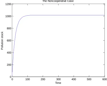
The pollution stock evolves according to the equation
𝑃𝑛𝑐∗ (𝑡) = 1.0133×10³ + 1.0335×10⁴𝑒−0.05𝑡 (50)
Figure 2: The optimal pollution stock evolution with no cooperation.
4.2 The cooperative scenario
For the cooperative transboundary pollution problem with emission trading, the optimal emission levels of the two countries are
𝐸𝑐𝑖∗(𝑡) = 50 − 3 − 5
0.15= 13.67 (51)
0 100 200 300 400 500 600
0 200 400 600 800 1000 1200
The Noncooperative Case
Time
P
o
llu
ti
o
n
s
to
c
𝐸𝑐𝑗∗ (𝑡) = 40 − 3 − 5
0.15= 3.67
The optimal number of emissions sold/bought by each country is as follows:
𝑌𝑐𝑖∗(𝑡) = 9.667
𝑌𝑐𝑗∗(𝑡) = −1.333
(52)
We remark that while country i is buying emission permits, country j has excess initial emission units that completely satisfy the optimal production schedule. Country j will therefore sell 1.333 units at each time t (under cooperation, country j does not buy any emission).
The revenues generated under the cooperation scenario could then be retrieved:
𝐽𝐶 = 771.1111 (53)
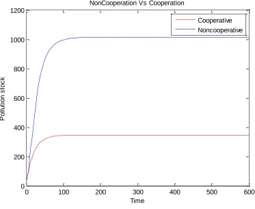
The pollution stock follows the equation below:
𝑃𝑐∗(𝑡) = 346.6667 + 2.2335×10⁴𝑒−0.05𝑡 (54)
Figure 3: The optimal pollution stock evolution with cooperation.
4.3 Comparison
After these results, we can compare the cooperative and non-cooperative scenarios to verify whether our findings are coherent with the numerical example. The difference in the emission strategies for countries i and j:
0 100 200 300 400 500 600
0 200 400 600 800 1000 1200
The Cooperative Case
Time
P
o
llu
ti
o
n
s
to
c
∆𝐸𝑖∗ = 𝐸𝑐𝑖∗ − 𝐸𝑛𝑐𝑖∗ = −20
∆𝐸𝑗∗ = 𝐸𝑐𝑗∗ − 𝐸𝑛𝑐𝑗∗ = −13.33
(55)
Countries that do not cooperate tend to release more emissions and produce more goods. The difference in emissions bought/sold by countries i and j are found as follows:
∆𝑌𝑖∗ = 𝑌𝑐𝑖∗(𝑡) − 𝑌𝑛𝑐𝑖∗ (𝑡) = 𝐸
𝑐𝑖∗(𝑡) − 𝐸𝑛𝑐𝑖∗ (𝑡) = −20
∆𝑌𝑗∗ = 𝑌𝑐𝑗∗(𝑡) − 𝑌𝑛𝑐𝑗∗ (𝑡) = 𝐸
𝑐𝑗∗(𝑡) − 𝐸𝑛𝑐𝑗∗ (𝑡) = −13.33
(56)
Now, the difference in the total discounted revenues (Cooperation vs Noncooperation) is
∆𝐽∗ = 𝐽
Figure 4: The optimal pollution stock evolution with and without cooperation.
4.4 With banking
The optimal emission strategy for the countries i and j remain unchanged as the noncooperative case,
𝐸𝑏𝑖∗ (𝑡) = 𝐴𝑖 − 𝜌 − 𝐷𝑖̇
𝑟 + 𝜃= 33.67 (58)
0 100 200 300 400 500 600
0 200 400 600 800 1000 1200
NonCooperation Vs Cooperation
Time
P
o
llu
ti
o
n
s
to
c
k
𝐸𝑏𝑗∗ (𝑡) = 𝐴𝑗− 𝜌 −
𝐷𝑗̇
𝑟 + 𝜃= 17.00
We now determine the optimal saving strategy for the countries i and j. For that let’s compute
the critical point
𝐿𝑐𝑟𝑖𝑡𝑖𝑐𝑎𝑙 = 𝑟 + 𝛾 − 1
𝑟 + 𝛾 =
0.1
1.1= 0.09 (59)
As a result, as 𝐿𝑖 = 0.08 < 𝐿𝑐𝑟𝑖𝑡𝑖𝑐𝑎𝑙 and 𝐿𝑗 = 0.12 > 𝐿𝑐𝑟𝑖𝑡𝑖𝑐𝑎𝑙 , country i will not be interested
in banking and 𝑆𝑖∗(𝑡) = 0, ∀𝑡 and 𝐵𝑖∗(𝑡) = 0, ∀𝑡. On the contrary, country j will be interested in banking and 𝑆𝑗∗(𝑡) = 20, and 𝐵𝑗∗(𝑡) = 20(1 − 𝑒−𝑡).
The optimal pollution stock remains the same as in the noncooperative case, namely,
𝑃𝑏∗(𝑡) = 1.0133×10³+ 1.0335×10⁴𝑒−0.05𝑡 (60)
The optimal number of emissions sold/bought by each country remains the same for country i
but changes for country j,
𝑌𝑏𝑖∗(𝑡) = 29.67
𝑌𝑏𝑗∗(𝑡) = 17.00 + 20 − 20(1 − 𝑒−𝑡) − 5 = 12 + 20𝑒−𝑡
(61)