The Characterization and Impact of Fluidized Zone Geometry and the Application of Impinging Jet to Estimate Soil Erosion.

ABSTRACT

KEBEDE, YULIAN ABAY. The Characterization and Impact of Fluidized Zone Geometry and the Application of Impinging Jet to Estimate Soil Erosion. (Under the direction of Dr. Mohammed A. Gabr).

The Characterization and Impact of Fluidized Zone Geometry and the Application of Impinging Jet to Estimate Soil Erosion

by

Yulian Abay Kebede

A thesis submitted to the Graduate Faculty of North Carolina State University

in partial fulfillment of the requirements for the degree of

Master of Science

Civil Engineering

Raleigh, North Carolina 2014

APPROVED BY:

_______________________________ ______________________________ Mohammed A. Gabr, PhD Roy Borden, PhD

Committee Chair

DEDICATION

BIOGRAPHY

Yulian Abay Kebede was born in Addis Ababa, Ethiopia to Abay Kebede Gebremariam (Father) and Elfinesh Tuffa Debele (Mother). After completing his secondary education at Dandii Boru School, located in his home town, he decided to pursue high school education in

the United States and enrolled at the Piney Woods School, located in Piney Woods, Mississippi. Yulian continued to receive his Bachelor of Science in Civil Engineering in May

2012 from Jackson State University located in Jackson, Mississippi. In August 2012, Yulian enrolled in the Masters of Science program with an emphasis in Geotechnical Engineering at North Carolina State University. Yulian plans to practice as a geotechnical engineer in the

ACKNOWLEDGMENTS

I would like to begin by thanking my professor and academic adviser, Dr. Mo Gabr, for his patience and continued guidance through my graduate studies. I would also like to thank my committee members and professors Dr. Brina Montoya and Dr. Roy Borden for their continued support.

I would like to thank my friend and fellow graduate student, Mohammad Kayser, for his help and contribution towards this research project. I would also like thanks to William Ruff, Ian McMillan, Shawn Anderson, Hamed Mousavi, Jinfu Xiao and Casey Shanhan for their assistance in various areas of this research project. Special thanks for Jerry Atkinson the all the staff members at the Constructed Facilities Laboratory.

NCDOT has offered a great deal of support for this project by offering test sites and improvement ideas. I would like to thank Mohammed Mulla for facilitating our relationship with NCDOT and for the design and fabrication of various ISEEP parts. I would also like to thank Pablo Hernandez and Wayne Currie for their logistical support when performing field tests in their regions.

TABLE OF CONTENTS

LIST OF TABLES ... vii

LIST OF FIGURES ... viii

CHAPTER 1: INTRODUCTION ...1

1.1: BACKGROUND ...1

1.2: OBJECTIVE ...2

CHAPTER 2: LITRATURE REVIEW ...3

CHAPTER 3: METHODOLOGY AND DATA REDUCTION ...11

CHAPTER 4: LABORATORY AND FIELD EXPERIMENTS ...16

4.1: LABORATORY EXPERIMENT ...18

4.2: ISEEP FIELD EXPERIMENT ...22

CHAPTER 5: NUMERICAL MODELING AND LABORATORY RESULTS ...26

5.1: NUMERICAL MODELING ...26

5.1.1: SCOUR MODEL ...26

5.1.2: SIMULATION DOMAIN ...29

5.1.3: NUMERICAL MODELING RESULTS ...31

5.2: FLUIDIZATION ZONE GEOMETRY...33

5.3: SKIN FRICTION REDUCTION...41

CHAPTER 6: FIELD RESULTS AND APPLICATION...47

CHAPTER 7: SUMMARY AND CONCLUSIONS ...59

LIST OF TABLES

Table 4.1: Test Soil Properties ...18

LIST OF FIGURES

Figure 1.1: Illustration of Scour Damages...1

Figure 2.1: Vertical Jet Apparatus & Resulting Stresses ...6

Figure 3.1: Penetration Depth vs. Time Plot ...12

Figure 3.2: Penetration Rate vs. Stream Power Plot ...14

Figure 4.1: Stainless Steel Probe w/t Sheathing & Tip ...16

Figure 4.2a: Pump-Tank Connection...17

Figure 4.2b: ITT PumpSmart Controller ...17

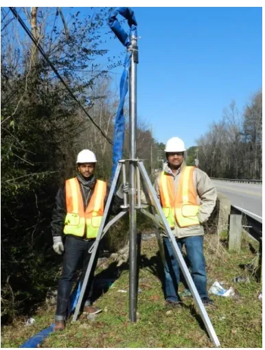
Figure 4.3: The ISEEP Device during Field Testing ...17

Figure 4.4: Plan View of Horizontal Test Setup ...19

Figure 4.5a: Cross Sectional View of Horizontal Test Setup A ...20

Figure 4.5b: Cross Sectional View of Horizontal Test Setup B ...20

Figure 4.6: Cross Sectional View of Vertical Test Setup ...21

Figure 4.7a: Map View of Jennette’s Pier Test Site...23

Figure 4.7b: Satellite view of Jennette’s Pier Test Site ...23

Figure 4.8: Jennette’s Pier ...24

Figure 4.9: Nortek Acoustic Scour Monitor Illustration ...24

Figure 4.10: Grain Size Distribution for Jennette’s Pier Soil ...25

Figure 5.1: Discretized Domain for Fluidization Zone Geometry Simulation...30

Figure 5.2a: Numerical Simulation of Fluidization Development with Time a t 10 sec...32

Figure 5.2d: Numerical Simulation of Fluidization Development with Time at 90 sec...32

Figure 5.3: Stress Contour at Jet Velocity of 2.3 m/s ...34

Figure 5.4: Stress Contour at Jet Velocity of 2.7 m/s ...34

Figure 5.5: Stress contour at jet velocity of 3.8 m/s ...35

Figure 5.6: Stress contour at jet velocity of 4.2 m/s ...35

Figure 5.7: Stress contour at jet velocity of 4.5 m/s ...36

Figure 5.8: Vertical Fluidization Phases at 2.4 m Probe Embedment ...38

Figure 5.9: Horizontal Fluidization Phases at 0.8 m Probe Embedment...38

Figure 5.10: Vertical Expansion of Fluidization Zone ...40

Figure 5.11: Attachable External Probe Weight with Handle ...45

Figure 5.12: Attachable Probe Weight Being Used as an Extraction Handle ...45

Figure 5.13: Reduced vs. Unreduced Skin Friction Forces at 6 m/s Jet Velocity ...46

Figure 6.1: Penetration Rate vs. Stream Power Plot for Jennette’s Pier ...47

Figure 6.2: Hourly Water Depths and Corresponding Wave Heights ... 48

Figure 6.3: Wave Period vs. Wave Height at Jennette’s Pier... 49

Figure 6.4: Erosion Rate vs. Wave Period for Varying Wave Heights (Top Layer) ...53

Figure 6.5: Erosion Rate vs. Wave Period for Varying Wave Heights (Bottom Layer) ....54

Figure 6.6: Wave Height vs. Erosion Duration for 5.5 meters Erosion Depth (Top Layer) ...57

Figure 6.8: Wave Height vs. Erosion Duration for 1 meter Erosion Depth

(Top Layer) ...58 Figure 6.9: Wave Height vs. Erosion Duration for 1 meter Erosion Depth

CHAPTER 1 INTRODUCTION

1.1 BACKGROUND

1.2 OBJECTIVE

Understanding the fluidization zone geometry along with the effect that it has on the penetration of the ISEEP probe is needed to refine the data analysis process of the ISEEP methodology and make it a more effective tool. The mapping and characterization of deep impinging jet fluidization zone geometry in an effort to calculate the magnitude of skin friction reduction that occurs during the penetration of the ISEEP probe is the primary objective of this research. Validation of the ISEEP testing and data reduction methodology was also another objective of this research. This was achieved through comparison of the ISEEP’s predicted scour values with measured scour values recorded from a single storm

event in the coast of North Carolina.

CHAPTER 2 LITRATURE REVIEW

Major forms of soil erosion include surface erosion, mass erosion, and fluidization as presented, for example, by Partheniades (1965) and Mehta (1991). During bed erosion, all three modes may be present in some proportion, though one typically dominates (Mehta, 1991). For coarse, non-cohesive materials, surface erosion occurs when the applied shear stress is at or above the sediment’s critical shear stress. For surface erosion, Briaud et al

(2001) reported the dominant means of particle motion (erosion) are sliding, rolling, and plucking. For cohesive soils, much of the erosion occurs in a process known as mass erosion. In mass erosion, material is transported away from the bed in the form of flocs or pods (cohesive groups) of grains. The rate of surface erosion also increases with the app lied shear stress. Partheniades (1965) identified the macroscopic shear strength of the bed at which the sediment can fail along an entire plane below the surface, allowing all of the material above the failure plane to be transported downstream. Briaud et al (2001) and Seed et al (2006) reported that sands may erode at rates of 10,000 mm/hr versus clay-type soils that may erode at 1 to 1,000 mm/hr.

maximum scour depth as the jet is held stationary on the surface. There is, however, a need for a better documentation of the erosion behavior produced by a jet that is embedded internally to the material. Niven and Khalili (1998a, 1998b, 2001, and 2002) discussed the mechanics and application of vertical, internal jets in a series of papers with their analysis mainly concerned with in situ fluidization of sand beds for environmental site remediation. In this case, the internal diameter of the jet was 75 mm and it was operated at relatively high flow rates on the order 5-13 l/s (80-206 gpm). They showed that jet penetration depth (fluidization zone depth) is proportional to the jet velocity and is a function Froude number.

Soil erodibility is defined as the rate of erosion that soil continues to experience once erosion process begins. This property is used to measure and predict erosion rates for different soil types. In the case of a vertical impinging jet, when fluid exiting the jet impacts the soil with a high enough velocity to induce shear stress higher than the soils shear strength, the flow is able to displace the local soil causing erosion. Vertical jetting techniques have been researched in relation with erosion; nevertheless, the main focuses of these studies a re scour depth and scour geometry not scour rate Chatterjee et al (1994).

To be able to correlate jet flow velocity with the critical level of shear stress that needs to be applied in order to cause erosion, the following properties must be known:

Briaud (2001) reported that the critical shear stress and the average particle size of a particle are proportional and within an approximate value of one another. This observation agrees with the relationship developed by Shields (1935) shown in Equation 2.1.



Where:



D50 = Median Grain Size (mm)

The Shields (1935) equation was letter modified by Julien (1995) to represent a dimensionless critical shear stress as shown in Equation 2.2. It can be concurred that particle size distribution has a significant effect in determining the magnitude of critical shear stress with directly relates with the soil erodibility.



* =



u*

/[(



-



)d)]

Where: u*= Critical Shear Velocity m = Density of Fluid Mixture

s= Unit Weights of the Sediment

mUnit Weights of the Fluid Mixture

The use of water jets in the study of erosion and scouring can be traced back as early as Rouse (1939). From the early studies of scour and water jets, it can be concluded that scour can be directly correlated with jet velocity and the depth of erosion caused by the water jets can be considered as scour (Utley, 2008). Hanson and Simon (2001) performed an analysis and determined that the commonly shields (1939) diagram, derived from Equation 2.1, overly conservative when used to determine critical shear stress for cohesive soils. Soon after, Hanson and Cook (2004) presented the resulting stress distribution from impinging jet as shown in Figure 2.1.

"Potential core" is the part of the jet where water does not lose its initial velocity. Once the potential core distance has been achieved by the water jet, a linear loss of velocity with distance occurs. The relationship between the applied shear stress and the potential core distance is expressed as follows:



Where:



U0 =Average jet velocity (m/s)

Water Density (kg/m3

),

Cf =Friction coefficient = 0.00416





Where:



Zp = Erosion Depth < Potential Core Depth

Zt = Total Scour Depth



E = kd (c(Mehta, 1991)   Equation 2.5

Where:  = Erosion Rate

Kd = Detachment Coefficient



Applied Shear Stress >

The detachment coefficient (Kd) is the normalized erosion rate with respect to shear stresses

exceeding the critical shear stress value hence, causing erosion. This erosion analysis method can be found as ASTM standard D5852.

The concept of stream power to measure the magnitude of the induced flow erosive potential was introduced by Annandale (1995). This concept is able to better predict turbulent flow regimes. Annandale (2006) also expressed P in terms of shear stressEquation2.6for the

case of impinging jet and indicated that such an approach accounts for the near boundary turbulent effect and should be used for reducing data from the impinging jet configuration. Based on derivations from the boundary layer theory, Annandale (2006) recommended that the Cf (Equation 2.3) to estimate the shear stress value is taken equal to 0.016.

P = qH = Uo (Annandale, 2006) Equation 2.6

Where: P =Stream Power (Watts/m2)

(1 Watt = 1 N*m per sec or Kg*m2 per sec 3)

= Unit Weight of Water

q = Discharge per Unit Area H = Energy Head

Internal fluidization is defined as the process in which granular soils behave fluid- like due to the loss of shear strength (Alsaydalani and Clayton, 2013). The study of internal fluidization can be applied in various geotechnical scenarios such as Leakage from water distribution pipes (Van Zyl et al, 2013); leakage through the clutches of sheet piles (Cashman and Preene, 2001); jetting tp facilitate pile penetration (Tsinket, 1988) and Jetting to aid jack-up spudcan extraction (Purwana et al., 2011). Granular materials are the focus of fluidization research because they are most susceptible to fluidization; other soil types are more resistant to fluidization due to the nature of their chemical composition.

CHAPTER 3

METHODOLOGY & DATA REDUCTION

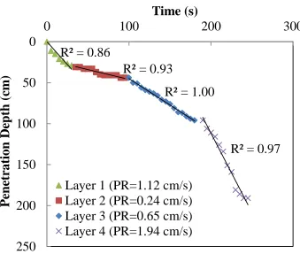
In previous publications, Gabr et al. (2013) evaluated critical stream power value by extrapolation stream power value from the penetration rate versus stream power plot assuming a linear relationship between penetration rate and stream power. It was later determined that the critical stream power value obtained through this linear relationship assumption ends up being much different than the critical stream power values published by other researchers. This is because the relationship between pe netration rate and stream power plots as a curve as opposed to being linear (Kayser, 2014). The corrected ISEEP data analysis and calculation method is presented as follows:

STEP 1 - Obtaining Penetration Rates For Different Laye rs:

Figure 3.1: Penetration Depth vs. Time Plot (Kayser, 2014)

STEP 2 - Calculate Applied Bed Shear Stress:

Shear stress produced by the jet, bed shear stress, can be calculated using Equation 2.3.

STEP 3 – Calculate Stream Powe r:

R² = 0.86

R² = 0.93

R² = 1.00

R² = 0.97

0

50

100

150

200

250

0

100

200

300

P

en

etr

at

ion

De

p

th (c

m

)

Time (s)

STEP 4 – Calculate Critical Stream Powe r:

Critical stream power, the minimum stream power required to begin the erosion process, can be obtained by multiplying the critical shear stress with the critical velocity as shown in Equation 3.1.



c c c

P  v (Briaud,Kayser, 2014) Equation 3.1

Where, *_cD_{50 }  (Briaud, Kayser, 2014)

v_c 0.35(D₅₀)0.45_{ }(Briaud,Kayser, 2014)

[*

τ

ν

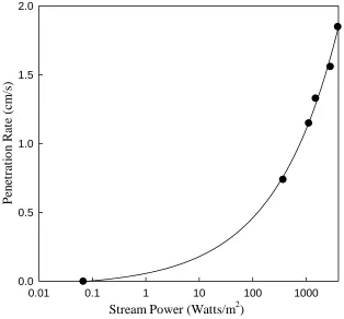
STEP 5 – Generate Stream Power Versus Penetration Rate Plot:

 

Figure 3.2: Penetration Rate versus Stream Power Plot (Kayser, 2014) 

STEP 6 – Calculate Detachment Rate Coefficient:

Detachment rate coefficient (kd') is a function of the applied stream power. For an

applied stream power value,k_d'can be obtained by calculated from the slope of the

erosion rate versus stream power plot that corresponds to the desired stream power. Stream Power (Watts/m2)

0.01 0.1 1 10 100 1000

STEP 7 – Calculate Erosion Rate:

The rate of erosion describes the mass rate of erosion per unit area. Erosion rate (E) as a

function of stream power exceeding the critical stream power value (Pc) can be calculated

using Equation 3.2.

E = kd’ (P - Pc) (Mehta, 1991; Kayser, 2014) Equation 3.2

Where: E = Erosion Rate

kd’ = Detachment Rate Coefficient

P = Applied Stream Power Pc = Critical Stream Power

STEP 5 – Calculate Erosion Magnitude:

CHAPTER 4

LABORATORY AND FIELD EXPERIMNETS

Figure 4.2a: Pump-Tank Connection Figure 4.2b: ITT PumpSmart Controller

4.1: LABORATORY EXPERIMENT

All laboratory tests was conducted in a liquefiable circular sand pit with a diameter of approximately 3m (9.5 ft) and a depth of 6 m (20 ft); Figure 4.1, Figure 4.2 and Figure 4.3 show the ISEEP device and all other attachments. Located within the lowest 0.46 m (18 in) of the pit, one water inlet and one drain outlet are placed for the purpose of infusing and draining water to regenerate the sand bed. These lie within a filter bed consisting of 0.23m (9 in) of #57 stone overlain by 0.23 m (9 in) of 'pea' gravel. The test sand originates from a quarry at Drowning Creek near Hoffman, NC, and is quartzite sand that was mined from an underwater alluvial deposit. Table 4.1 shows the soil and soil interaction properties.

Table 4.1: Test soil Properties (Kebede et al, 2014)

Total Unit Weight (kN/m3) γ 17.8

Median soil grain size (mm) D50 0.3

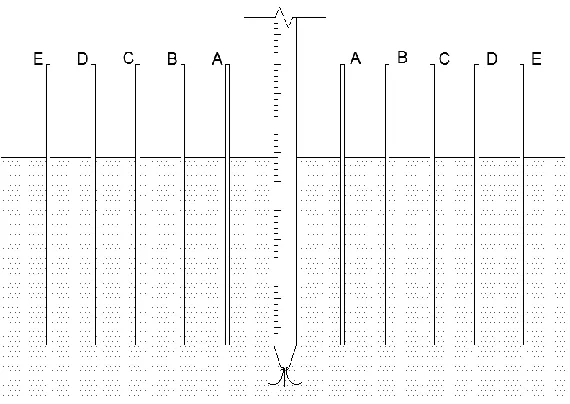
Two sets of experiments were performed to capture the geometry of the fluidization zone. The first experiment was performed by embedding thin transparent tubes around the probe at different depths in order to capture the lateral expansion of the fluidization zone. In this case, 15 thin transparent tubes with inner diameter of 3.175 mm (1/8 in) and outer diameter of 6.35 mm (1/4 in) were vertically embedded around the probe as shown in Figures4.4 and Figure 4.5. The tube embedment depth varied from 0.4m to 1.2m. The water levels in the tube were monitored throughout the test; this data was used to calculate the effective stress at the bottom of each tube which was then used to determine whether or not the soil at that location is fluidized. The exit velocity was varied from 2.3 m/s up to 5.1 m/s for these groups of tests, and the probe was held stationary at a known depth while each test was performed.

A B C D E A B C D E A B C D E

LINE 3 LINE 1

LINE 2

Diameter = 3m (10ft)

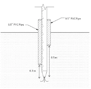
The second experiment was aimed to capture the vertical expansion of the fluidization zone. This experiment was conducted by attaching two and four piezometers at different depths onto the probe as shown in Figure 4.6. PVC pipes (12.3 mm in diameter) were used as the piezometers for these tests. A Geokon 500 water level meter was used to measure the water level in the piezometers during testing at certain time intervals. These measurements were also recorded and used to calculate the effective stress at each depth at a given time and monitor the vertical expansion of the fluidization zone. The water exit velocities were varied from 4.2 m/s to 6.0 m/s for these groups of tests, and the probe was held stationary at a known depth (Kebede et al, 2014).

Figure 4.6 illustrates the test setup; in this experiment, four piezometers were directly attached to the walls of the probe and jetted down to a desired depth of 2.4 m. The probe was then fixed at that depth and testing was performed 24 hours after the jetting process in order to dissipate the jetting effect and allow the soil to settle. Three different tests were performed for three different jet velocities of 4.2 m/s, 5.1 m/s, and 6.0 m/s (Kebede et al, 2014).

4.2: ISEEP FIELD EXPERIMENT

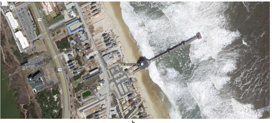
Field testing with the ISEEP was conducted at various locations throughout the state of North Carolina. These tests were conducted in both coastal and inland locations that are susceptible to erosion. This section presents a set of field experiments performed with the ISEEP device at Jennette’s pier located in Nags Head, North Carolina. The results from these tests were

compared and contrasted with scour activity monitored using Nortek acoustic scour monitor installed at Jennette’s pier (Figures 4.8 and 4.9). This monitor was installed on a 0.6 m by 0.6 m square pier pilling on the seaward end of Jennette’s pier on January 24, 2013. Even though

a.

Figure 4.7: (a.) Map View of Jennets Pier Test Site (Source: Google Maps)

b.

25 Soil samples from the site were collected and grain size distribution test was performed in the laboratory to classify the collected soil. As shown in figure 4.10, it was determined that the average grain size distribution (D50) was 0.25mm for the top layer and 0.3mm for the bottom

layer.

Figure 4.10: Grain Size Distribution for Jennette’s Pier Soil (Kayser, 2014)

0

10

20

30

40

50

60

70

80

90

100

0.01

0.1

1

10

P

erc

ent

P

assi

ng

Grain Size (mm)

Top Layer

CHAPTER 5

NUMERICAL MODELING AND LABORATORY RESULTS

5.1: NUMERICAL MODELING

The CFD software, FLOW-3D, is used to perform numerical simulations for mapping fluidization zone geometry. FLOW-3D (2011) is based on the fundamental laws of mass, momentum and energy conservation. It simulates the flow process using the standard Navier-Stokes flow equation. The domain is discretized using finite difference b locks, and the governing equation is solved for each computational cell. The fractional area-volume obstacle representation (FAVOR) method is utilized for modeling solid obstacles within the domain (Hirt and Sicilian, 1985; Kayser and Gabr, 2013).

5.1.1: SCOUR MODEL

The input parameters of the sediment scour model are: diameter and density of the sediment (d, ρ), the critical Shields parameter, entrainment coefficient (Ce), drag coefficient (Cd), bed

load coefficient (Cb) and angle of repose (Φ) (Kayser and Gabr, 2013). When the critical

Shields parameter is not assigned during the numerical simulation, FLOW-3D calculates the value from the Shields curve (Brethour and Burnham, 2010). The definitions of Ce, Cd, and

Cb are as follows:

1. Ce describes the lifting of the sediment in the bulk flow of fluid. According to FLOW-3D

(2011), the entrainment coefficient predicts the rate of sediment erosion at a shear stress higher than the critical shear stress (Kayser and Gabr, 2013).

2. Cd quantifies the resistance of the sand particles to the fluid flow (Kayser and Gabr, 2013).

Engelund and Hansen (1967) proposed Equation 5.1 for natural sands and gravels based on laboratory measurements:

Cd=

+ 1.5 Equation 5.1

3. Cb is related to the transport of heavy particles along the top of the packed bed by the flow

of water; in this process, the bed load coefficient is used to predict the rate of transport at a shear stress higher than the critical shear stress (Kayser and Gabr, 2013). The default value of the bed load coefficient is 8.0 in FLOW-3D (2011) following the Meyer-Peter and Muller (1948) equation. Nnadi and Wilson (1992) reported a Cb value of 12 for a sheet flow regime,

and Ribbernik (1998) suggested a Cb of 5.7 for bed load data that are very close to the incipient motion. A typical Cb value for sand and gravel is 5.7 (Ribbernik, 1998), (Fernandez

and Beek, 1976), (Kayser and Gabr, 2013).

Table 4.2 provides values of the different parameters used for sandy soil. These value ranges are used as input parameters in the sediment scour model. As explained earlier, the ‘Critical Shields Parameter’ value cell is blank in the table for the numerical simulations because the

number is computed from the Shields curve (Brethour and Burnham, 2010). The Cd value

was varied from 1.0 to 2.0 (Rubby, 1933); (Wu and Wand, 2006), the Ce value was varied

from 0.009 to 0.036, and the Cb value was varied from 4 to 8; these ranges are assumed based

Table 5.1: Parameter Values Used in Numeric Simulations (Kayser and Gabr, 2013)

Parameter Value

Density, ρ 1500 Kg/m3

Entrainment Coefficient, Ce 0.009 to 0.036

Drag Coefficient, Cd 1 to 2

Bed Load Coefficient, Cb 4 to 8

Angle of Repose, Φ 31o

5.1.2: SIMULATION DOMAIN

0.7 m

0.7 m

2.0 m

5.1.3: NUMERICAL MODELING RESULTS

(a) (b)

5.2: FLUIDIZATION ZONE GEOMETRY

Effective stress and pore-water pressure values for recorded time intervals were calculated using the soil properties and the experimental data. By designating zero effective stress as a state of total fluidization, the fluidized zone is estimated. To better visualize and understand the horizontal expansion of the fluidization zone, stress contours were generated. The horizontal and vertical axis of these stress contours represent the horizontal and vertical distances from where the probe is vertically embedded into the soil. The color-filled contour map shows the effective stress of the soil at a time where the fluidization bulb forming around the probe reaches steady state, having no further expansion. This time was observed to be greater than 15 minutes (Kebede et al, 2014). The stresses are measure in Pascal (Pa) units and the legends for the contour colors are given on the right side of each stress contour figure.

Figure 5.5: Stress Contour at Jet Velocity of 3.8 m/s (Kebede et al, 2014)

Results from the contour maps illustrate the fluidization zone with increased depth and increased jet velocity. The fluidized zones shown in Figure 5.3 and Figure 5.4 appear to be similar since the increase in the jet velocity is not enough to cause a significant amount of change. After increasing the embedment depth and the jet velocity, a more noticeable expansion in the fluidization zone can be observed in Figure 5.5, Figure 5.6 and Figure 5.7. A jet velocity of 3.8 m/s causes a maximum lateral distance of the fluidization zone that extends 0.3 m from the probe. At jet velocities of 4.2 m/s and 4.5 m/s, the lateral distance of

As explained in the previous section, a different test setup was used to study the vertical expansion of the fluidization zone. Figure 5.8 shows the effective stress versus time recorded at the probe embedment of 2.4 meters below ground surface. These results are used to understand the vertical advancement of the fluidization zone above the jet. Since the horizontal and vertical fluidization zone expansions were studied in two different types of laboratory tests, the results were plotted in separate plots. Figure 5.9 shows the effective stress versus time relationship; but, since the test was ran for a shorter time, only the initial and the transitional phases were able to be shown. Figure 5.8 shows results for fluidization experiments that were able to be continued for an extended amount of time; thus, the phase changes can be clearly observed.

Figure 5.8: Vertical Fluidization Phases at 2.4 m Probe Embedment (Kebede et al, 2014)

4500 5000 5500 6000 6500

60 110 160 210 260 310 360

Effe

ct

ive

St

re

ss

(P

a)

Time (Sec)

From Figure 5.8, the rate of change of the effective stress with time can be categorized to three different phases. The initial phase can be seen as the linear drop starting from the initial time down to where the curve begins to form. This phase represents the formation of a fluidization zone as the jet fluidizes the soil around it. The second phase, which is referred to as the transition phase, occurs when the curve is forming after the sharp drop o f effective stress in the initial phase. This zone demonstrates the gradual increase of the fluidization zone before it reaches its limit. The final phase, which is also referred to as the steady state phase, can be seen as the change in the effective stress gradually decreases and approaches a horizontal line. This phase happens when the fluidization zone has reached its maximum dimensions and is no longer expanding.

Looking at the 1.5 m zone, the 5.1 m/s jet velocity is at the 95% confidence zone, showing that it is very close to the fluidization threshold. The probe tip is located at an embedment depth of 2.44 meters below ground surface in Figure 5.10.

5.3: SKIN FRICTION REDUCTION

The term skin friction also known as side friction is commonly used to refer to the frictional resistance developed between a pile and adjacent soil in an embedded pile foundation system. This frictional resistance along with the toe bearing is utilized to transfer the superstructure load (column load) into the soil. Skin friction ana lysis can be performed using two methods:

1. Total stress analysis also known as the alpha (α) method 2. Effective stress analysis also known as the beta (β) method

Since the effective stress method has been proven to yield a more accurate result, the β-method (effective stress analysis) was used in all skin friction analysis throughout this thesis. The mechanics of skin friction can be described using a simple sliding- friction model as follows:

Fs = σ’h tanϕint Equation 5.2

Where: Fs Skin friction resistance σ’h Horizontal effective stress

= Ka * σ’vertical

Ka Lateral earth pressure (active)

= tan2 (45 - ϕ’ )

ϕint soil-pile Interface effective friction angle

Various studies have been done to better understand interface friction values in the case of an object such as a pile is penetrated into soil. Kulhawy et al (1983) and Kulhawy (1991) suggest that the interface friction angel between a smooth steel surface and surrounding soil equals half of the soil’s effective internal friction angle. To calculate the horizontal effective stress, the lateral earth pressure is multiplied by the vertical effective stress. Kulhawy et al (1983) and Kulhawy (1991) suggests that the coefficient of lateral earth pressure to be reduced by a factor of 0.5 – 0.7 to account for the loosening of the nearby soil due to the jetting effect. After considering these adjustments, the skin friction can be rewritten as follows:

Fs = σ’v* Ko * *tan [ϕ’] Equation 5.3

Where:

Lateral earth pressure reduction factor

= 0.5 for the ISEEP case

Interface friction reduction factor

Using Equation 5.3, a corrected skin friction is calculated and compared with the un-reduced skin friction value in Figure 5.12 and Table 5.1. All the corrected skin friction values shown in Figure 5.12 were generated from the fluidization zone experiment that was presented in Chapter 4 of this thesis. Vertical piezometers were used to monitor the advancement of the fluidization zone. Figure 5.10 illustrates the amount of skin friction reduction that occurs as the fluidization zone forms and expands until reaching the steady state phase. The presented data was calculated from tests performed at 1.2 meter probe embedment depth and 2.4 meter embedment depth with a jet velocity of 6 m/s.

As shown on Figure 5.12, a significant amount of skin friction reduction can be seen throughout the entire test. In comparison of the unreduced skin friction forces with the reduced values, the following conclusion can be made:

1. During the initial fluidization phase at jet embedment of 1.2 meters, a skin friction force reduction of approximately 5 Newton is calculated. This accounts for a 30% reduction of skin friction.

3. During the initial fluidization phase at jet embedment of 1.2 meters, a skin friction force reduction of approximately 17.3 Newton is calculated. This accounts for a 100% reduction of skin friction.

4. During the initial fluidization phase at jet embedment of 2.4 meters, a skin friction force reduction of approximately 3 Newton is calculated. This accounts for a 4% reduction of skin friction.

5. During the transition fluidization phase at jet embedment of 2.4 meters, a skin friction force reduction of approximately 11 Newton is calculated. This accounts for a 17% reduction of skin friction.

6. During the steady state fluidization phase at jet embedment of 2.4 meters, a skin friction force reduction of approximately 21.2 Newton is calculated. This accounts fo r a 31% reduction of skin friction.

Knowing the skin friction value experienced by the ISEEP probe as it penetrates into the sub-surface can be used to calculate the amount of weight that needs to be added on to the probe to achieve a smooth penetration while testing is being conducted. This handle shown in Figure 5.10, is made out of stainless steel and has a weight of approximately 15 Kg, same as the weight of one probe section. This weight also serves as an ext raction handle to pull out the probe after the completion of a penetration test as shown in Figure 5.11.

Figure 5.11: Attachable External Probe Weight with Handle

Table 5.2: Tabulated Values for Reduced and Unreduced Skin Friction Forces at 6 m/s Jet Velocity

Probe Embedment Depth Fluidization Zone Height Skin Friction Force

Unre duced Skin Friction Force

z (m) Fluidized Fs (N) Fs (N)

Initial Phase

1.2 0.2 12.0 17.3

2.4 0.05 66.5 69.3

Transition Phase

1.2 0.4 7.7 17.3

2.4 0.2 58.3 69.3

Steady State Phase

1.2 1.2 0.0 17.3

2.4 0.4 48.1 69.3

0 10 20 30 40 50 60 70

1 1.5 2 2.5

S k in F ri ct ion F or ce ( N )

Probe Embedment (m) Initial Phase

CHAPTER 6

FIELD RESULTS AND APPLICATION

Following the ISEEP data reduction approach mentioned above, critical stream power and detachment rate coefficient values were obtained for the ISEEP field test performed at the Jennette’s Pier test site. Figure 6.1 shows the applied stream power values versus penetration rate values. The detachment rate coefficient (kd’) was then calculated for a corresponding

stream power value using a straight line portion of the curves given in Figure 6.1.

Figure 6.1: Penetration Rate vs. Stream Power Plot for Jennette’s Pier (Kayser, 2014) 0 1 2 3 4 5 6 7 8 9 10

0.01 0.1 1 10 100 1000 10000

P en et rat ion R at e ( cm /s )

Stream Power (Watt/m2₎

Top La yer

Figure 6.3: Wave Period vs. Wave Height at Jennette’s Pier (Dubbs et al, 2014)

Jennette’s pier was conducted before this storm event, the predicted erosion estimations were

compared with the recorded erosion values.

All the wave data were taken from the recorded valued from March 6th 2013 to March 10th 2013.The maximum wave height recorded for this specific storm period was taken as 5 meters (Figure 6.3) and a corresponding wave period of 17 seconds. This was then used to calculate the wave length for the wave with the given height and period. The wave length equation, Equation 6.1, was used to calculate the wave length (Reeve etal, 2012).

(ω2

*d) / g = k*d tanh (k*d) (Reeve etal, 2012) Equation 6.1

Where: ω: Angular Frequency (rad/sec) = (2π) / T

T: Wave Period (sec) d: Water Depth (m)

g: Gravitational Acceleration k: Wave Number (rad/sec)

= (2π) / L

After calculating the wave length, the following step would be to calculate the maximum orbital wave velocity (Um) just above the boundary layer, the top of the bed soil. This can be

calculated using Equation 5.4 given below.

u

(Reeve etal, 2012) Equation 6.2

Where: Um: Maximum Velocity (m/sec)

H: Wave Height (m) T: Wave Period (Sec) d: Water Depth (m) L: Wave Length (m)

fw = 0.04 *

Where: fw: Wave Friction Factor

Um: Maximum Wave Velocity (m/s)

T: Wave Period (sec) kb: Bed Roughness Factor

= 3* D50

D50: Average Grain Size Distribution (mm)

τ

Where:

τ

After the applied bed shear stress is calculated, this value is then converted to a stream power value by using Equation 6.5.

P =

τ

Where: P: Applied Stream Power (Watts/m2)

τ

Um: Maximum Applied Wave Velocity (m/sec)

From this calculation, an applied stream power value can be obtained. The straight line plot for the corresponding stream power value from Figure 6.1 can now be used to calculate a kd’. This process was done for the top and bottom soil layers and corresponding detachment rate coefficient (kd’) values were obtained. Using the kd’ value along with Equations 3.1 and 3.2,

the rate of erosion for the Jennette’s pier at this specific storm event is calculated. The

Figure 6.4: Erosion Rate vs. Wave Period for Varying Wave Heights (Tope Soil Layer) 0.000 1.000 2.000 3.000 4.000 5.000 6.000 7.000 8.000

7 9 11 13 15 17

E ros ion R at e ( cm /s ec )

Wave Period (sec)

Wave Height = 5m

Wave Height = 4m

Wave Height = 3m

Wave Height = 2m

Figure 6.5: Erosion Rate vs. Wave Period for Varying Wave Height (Bottom Soil Layer) 0.000 1.000 2.000 3.000 4.000 5.000 6.000 7.000 8.000

7 9 11 13 15 17

Er os ion R at e ( cm /s e c)

Wave Period (Sec)

Wave Height = 5m

Wave Height = 4m

Wave Height = 3m

Wave Height = 2m

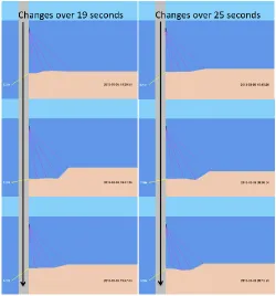
From Figure 6.2, a 5.5 meter of maximum erosion magnitude was reported for the March 6 2013 storm event (Dubbs et al, 2014). By converting the wave forces to stream power values, erosion rates were able to be calculated for the wave heights and wave periods that occurred within the storm period reported by Dubbs et al (2014). Figures 6.6 and 6.7 show the time it takes to causes a 5.5 meter of erosion depth which is the maximum amount of erosion that occurred during the reported storm event at Jennette’s pier. Figures 6.8 and 6.9 show the time it takes to cause a 1 meter erosion depth at Jennette’s pier for the recorded water wave characteristics. A 5.5 meters erosion depth could occur within 1.2 minutes at the top soil layer and 4.2 minutes at the bottom soil layer for maximum wave height and minimum wave period. A 1 meter erosion depth could occur within 15 seconds at the top soil layer and 55 seconds at the bottom soil layer for maximum wave height and minimum wave period.

Figure 6.6: Wave Height vs. Erosion Duration for 5.5 meters Erosion Depth (Top Layer)

Figure 6.7: Wave Height vs. Erosion Duration for 5.5 meters Erosion Depth (Bottom Layer)

0 1 2 3 4 5 6

0.001 0.010 0.100 1.000 10.000 100.000 1000.000

W av e H e ig ht ( m )

Erosion Duration (Hours)

Wave Period = 8 sec

Wave Period = 17 sec

0 1 2 3 4 5 6

0.001 0.010 0.100 1.000 10.000 100.000 1000.000

W av e H e ig ht ( m )

Erosion Duration (Hours)

Wave Period = 8 sec

Figure 6.8: Wave Height vs. Erosion Duration for 1 meter Erosion Depth (Top Layer) 0 1 2 3 4 5 6

0.001 0.010 0.100 1.000 10.000 100.000 1000.000

W av e H e ig ht ( m )

Erosion Duration (Hours)

Wave Period = 8 sec

Wave Period = 17 sec

0 1 2 3 4 5 6

0.001 0.010 0.100 1.000 10.000 100.000 1000.000

W av e H e ig ht ( m )

Erosion Duration (Hours)

Wave Period = 8 sec

CHAPTER 7

SUMMARY AND CONCLUSIONS

The objective of this research can be divided into two main categories:

1. The mapping and characterization of deep impinging jet fluidization zone geometry through laboratory tests and numerical modeling in an effort to calculate the magnitude of skin friction reduction that occurs during the penetration of the ISEEP probe.

2. Validation of the ISEEP testing and data reduction methodology by comparing the ISEEP’s predicted scour values with measured scour values from laboratory and field tests.

Laboratory test and numerical modeling results on jet induced vertical and horizontal fluidization zone at different depths are presented. Stress contours to map the geometric expansion of the fluidization zone are developed. Based on the results obtained in this study, the following conclusions are advanced:

is categorized as the steady state phase, is reached when there is no further effective stress reduction with time and is used herein to indicate the point when maximum fluidization zone is reached (Kebede et al, 2014).

ii. The size of the fluidized zone that was monitored with the laboratory tests linearly

proportional with the applied jet velocity. A jet velocity of 3.8 m/s resulted in a maximum lateral distance of the fluidization zone that extended 0.3 m from the probe. At jet velocities of 4.2 m/s and 4.5 m/s, the lateral distance of the fluidization zone reached about 0.40 m and 0.45 m, respectively (Kebede et al, 2014).

iii. The vertical extent of the fluid ized zone that was monitored in the laboratory was

approximately 15 times the jet diameter but also increased with the magnitude of the jet velocity; at a velocity of 4.2 m/s, it was measured as 0.3 m, and at jet velocities of 5.1 m/s and 6 m/s, the fluidization zone vertically extended 0.9 m above the jet tip (Kebede et al, 2014).

iv. At a depth of embedment of 2.4 m, this maximum fluidization zone occurs as a closed

fluidization. The dimensions of this zone are a function of the applied jet velocity (considering the values used in this study) (Kebede et al, 2014).

was concluded that a minimum runtime of 70 seconds is needed to achieve steady state fluidization. For a jet velocity of 4 m/s, the fluidization zone extended 0.3 meters above the probe tip and horizontally expanded with a radius of 0.25 meters. The obtained results matched closely with the laboratory experiment results; however, more simulations should be performed for a better understanding of the fluidization zone.

CHAPTER 8 FUTURE WORK

This thesis focused on laboratory and field tests in attempt to improve and validate the ISEEP device and methodology. The laboratory tests focused on understanding the fluidization geometry in order to better estimate the issue that skin friction has on the penetrat ion of the probe. As discussed in Chapter 3, multiple piezometers were inserted systematically around the probe at different depths in the soil to monitor the pressure as the fluidization zone expands. The water level in the piezometers was monitored visua lly by the author and other graduate students. The author highly recommends an automated monitoring system for future research in order to gather a more accurate data by eliminating human errors. The author was also limited in the number of piezometers since visual monitoring becomes very difficult as the number of tubes increase. An automated monitoring system can eliminate this issue and more piezometers or pressure sensors can be installed to improve the mapping of the fluidization zone. This could allow for the horizontal and vertical expansion of the bulb to be mapped in every test which will allow for a better understanding of the nature of expansion of the fluidization bulb.

Standardized Operation-Decisions” was submitted in response to DHS Center of Excellence Partners funding opportunity announcement (FOA).

Various modifications and improvements were made to the ISEEP device within the time frame of this research but more improvements are needed. The ISEEP probe has markings on its outer skin that is used to monitor the penetration rate. These marking usually are erased after one or two penetration tests. The author suggests a more permanent engraved markings the will potentially expedite testing time. The ISEEP pump and controller also has shortcomings and needs improvement. For the future, a smaller pump tha t offers a wider water output velocity can benefit the ISEEP field tests.

REFERENCES

Aderibigbe, O. and Rajaratnam, N. (1996). “Erosion of Loose Beds by Submerged Circular Impinging Vertical Turbulent Jets.” Journal of Hydraulic Research, 34(1), 19-33.

Alsaydalani, M. O. A., Clayton, C.R.I. (2013). “Internal Fluidization in Granular Soils.” Journal of Geotechnical and Geoenvironmental Engineering, 1090-241.

Annandale, G. W. and Parkhill, D. L. (1995). “Stream Bank Erosion: Application of the

Erodibility Index Method.” International Water Resources Engineering Conference - Proceedings, 2 1570-74.

Annandale, G.W. (2006). “Scour technology: mechanics and practice.” McGraw Hill, New

York. 430 pp.

Beltaos, S. and Rajaratnam, N. (1974). “Circular Turbulent Impinging Jets.” Journal of

Hydraulic Engineering, ASCE 100 (10), 1313-28.

Brethour, J., and J. Burnham.“Modeling Sediment Erosion and Deposition with the FLOW- 3D Sedimentation & Scour Model.”Flow Science Technical Note, FSI-10-TN85, 2010,

pp. 1-22.

Briaud, J. L., et al. (2001). “Erosion Function Apparatus for Scour Rate Predictions.” Journal of Geotechnical and Geoenvironmental Engineering, 127 (2), 105-13.

Briaud, J. L. (2002). TTI Researcher, V38, #4.

Chatterjee, S. S., S. N. Ghosh, and M. Chatterjee (1994). “Local scour due to submerged horizontal jet,” Journal of Hadraulic Engineering, 120, 973 – 992.

Dubbs, L., Edge, B., Gamiel, K. and Muglia, M. (2014). “Scour Monitoring in an Energetic Open Ocean Environment.” Proceedings of the 2nd

Marine Energy Technology Symposium.

Engelund, F., and E. Hansen,“A Monograph on Sediment Transport to Alluvial Streams.”

Copenhagen, Tenik Vorlag, 1967.

Fernandez, L. R., and R. Van Beek. Erosion and Transport of Bed-Load Sediment. Journal of Hydraulic Research, Vol. 14, No. 2, 1976, pp. 127-144.

FLOW-3D. (2011).User Manual. Flow Science, Inc.

Gabr, M., Caruso, C., Key, A. and Kayser, M. (2012). “Assessment of In Situ Scour Profile in Sand Using a Jet Probe.” Geotechnical testing journal, 36 (2), 0149-6115.

Hanson, G. J. and S. L. Hunt. (2007). "Lessons Learned Using Laboratory Jet Method to Measure Soil Erodibility of Compacted Soils." Applicatio n of Engineering in

Agriculture, 23 (3), 305-12.

Hanson, G. J. and K. R. Cook. (2004). "Apparatus, Test Procedures, and Analytical Methods to Measure Soil Erodibility in Situ", Ap. Engr. in Ag., 20 (4), 455-62.

Hanson, G. J., Robinson, K. M., and Cook, K. R. (2002). “Scour Below an Overfall: Part 2. Prediction.” Transactions of the American Society of Agricultural Engineers, 45 (4),

Hirt, C., and J. Sicilian.“A Porosity Technique for the Definition of Obstacles in Rectangular Cell Meshes.” In Proc. Fourth International Conf., Ship Hydro., National Academy of

Science, Washington, D.C., 1985.

Julien, P. Y. (1995). “Erosion and sedimentation.” Press Syndicate of the University of

Cambridge, New York, NY

Kayser, M. (2014). “Investigation of Soil Erodibility using In Situ Erosion Evaluation Probe

(ISEEP).” Doctoral Thesis, North Carolina State Univeristy, Raleigh, 126pp.

Kebede, Y. A., Gabr, M.A. and Kayser, M.F. (2014). “Scour Zone Characterization by Deep Impinging Jet.” Proceedings of the 33rd

international Conference on Ocean, Offshore and Arctic Engineering, San Francisco, California.

Kulhawy, Fred H. (1991). “Drilled Shaft Foundations.” Chapter 14 in Foundation

Engineering Handbook, 2nd ed., Hsai-Yang Fang, Ed., Van Nostrand Reinhold, New York

Kulhawy, F.H., Trautmann, C.H., Beech, J.F., O’Rourke, T.D., McGuire, W., Wood, W.A. and Capanco, C., (1983). ‘Transmission Line Structure Foundation for

Uplift-Compression Loading.” Report No. EL-2870, Electric Power Research Institute, Palo

Alto, CA

Mehta, A. J. (1991). “Review notes on cohesive sediment erosion In: N.C. Kraus, K.J. Gingerich, and D.L. Kriebel.” (eds.), Coastal sediment 1991, Proceedings of Specialty

Mehta, A., and Christensen, B. (1983). “Initiation of sand transport over coarse beds in tidal entrances.” Coastal Eng., 7, 61–75.

Meyer-Peter, E., and R. Mueller. “Formulas for Bed-Load Transport.” In. Proc. Second Meeting of the International Association for Hydraulic Research, IAHR, Stockholm, Sweden, 1948, pp. 39-64.

Niven, R. K. and N. Khalili. (1998). “In Situ Fluidization by a Single Internal Vertical Jet.”

Journal of Hydraulic Research, 36 (2), 199-228.

Niven, R. K. and N. Khalili. (1998). “In Situ Multiphase Fluidization (Up flow Washing) for the Remediation of Hydrocarbon Contaminated Sands.” Canadian Geotechnical Journal,

35 (6), 938-60.

Niven, R. K. (2001). “In Situ Fluidization for Solids Addition to Permeable Reactive

Barriers.” 2001 International Containment and Remediation Technology Conference and

Exhibition, Orlando, FL, June, 10-13.

Niven, R. K. and N. Khalili. (2002). “In Situ Fluidization for Peat Bed Rupture, and Preliminary Economic Analysis.” Journal of Contaminant Hydrology Research, 36(2),

199-288.

Nnadi, F. N., and K. C. Wilson. “Motion of Contact-Load Particles at High Shear Stress.”

Journal of Hydraulic Engineering, Vol. 118, No. 12, 1992, pp.

Partheniades, E. (1965). “Erosion and Deposition of Cohesive Soils.” Journal of the

Hydraulics Division, ASCE, 91 (1), 105-39.

Reeve, D., Chadwick. A. and Fleming, C. “Coastal Engineering: Processes, Theory and

Ribberink, J. S. “Bed-Load Transport for Steady Flows and Unsteady Oscillatory Flows.”

Coastal Engineering, Vol. 34, 1998, pp. 59– 82.

Rouse, H. (1939). “Criteria for Similarity in Transportation of Sediment.” State University of

Iowa, 33-39.

Rubey, W. Settling. “Velocities of Gravel, Sand and Silt Particles.” American Journal of

Science, Vol. 25, No. 148, 1933, pp. 325–338.

Tsinker, G. P. (1988). “Pile Jetting.” Journal of Geotechnical Engineering, 10.1061/(ASCE)

0733-9410(1988) 114:3(326), 326-334

Utley, B. C. and Wynn, T.M. (2008). “Cohesive Soil Erosion: Theory and Practice.” World Environment and Water Resources Congress 2008: Ahupa’a, May 12, 2008 – May 16,

2008, American Society of Civil Engineers, Honolulu, HI, United States, Environmental and Water Recourses Institute.

Van Zyl, J.E., Alsaydalani, M.O.A., Clayton, C.R.I., Bird, T., andDennis, A. (2013). “Soil Fluidization outside Leaks in Water Distribution Pipes Preliminary Observations.”

Proceedings Institute of Civil Engineering, Water Management, 166(10), 546-555. Vardoulakis, I., Stavropoulou, M. and Papanastasiou, P. (1996). "Hydro- mechanical aspects

of the sand production problem." Transport in Porous Media 22, 225–244.

Wu, W., and S. S. Y. Wang. Formulas for Sediment Porosity and Settling Velocity. Journal of Hydraulic Engineering, Vol. 132, No. 8, 2006, pp. 858-862.

Yakhot, V., and S.A. Orszag. “Renormalization Group Analysis of Turbulence. I. Basic