FUNFITS data analysis and statistical tools for estimating functions

't

<':1.'"

,

...-: r~;::!'\_

.

,

.

--.;

FUNFITS: Data Analysis and Statistical Tools

for Estimating Functions

Douglas Nychka, Barbara Bailey and Stephen Ellner

Perry Haaland and Michael O'Connell

Institute of Statistics Mimeo Series #2289

(~----)

I

Mimeo Series # 2289 I

FUNFITS, Data Analysis and II Statistical Tools for Estimating

Functions .I

i

Douglas Nychka, Barbara Bailey,

1

and Stephen Ellner, Perry Haaland

1

and Michael O'Connell

1

'---:::-

-=-~I

I

I: Kame Date f

I

: I

l

I

i

I

I

J

;;:-'"

;:,

...

...

...

FUNFITS: data analysis and statistical tools for

estimating functions

Douglas Nychka, Barbara Bailey and Stephen Ellner*

North Carolina State University

Perry Haaland and Michael O'Connell

Becton Dickinson Research Center

Abstract

A module of functions has been created to simplify and extend the fitting of curves and surfaces to data. Some important applications include estimates of the mean value of a measured response over some space of interest, response surface methods for designed experiments and the modeling of nonlinear dynamic systems. The core methods that are implemented in FUNFITS include prediction, plot and summary functions that help the user interpret results and visualize the estimate. FUNFITS is written mainly in the S programming language with some support from FORTRAN subroutines. All sourceisavailable and easy to modify.

Contents

1 Introduction

2 What's so special about FUNFITS?

2.1 An example .

3 A Basic model for regression

4 Thin plate splines: tps

4.1 Determining the smoothing parameter

4.2 Approximate splines for large data sets .

4.3 Standard Errors. . . .

5 Spatial process models: krig

5.1 Specifying the Covariance Function.

5.2 Some examples of spatial process estimates.

6 Generalized ridge regression

6.1 Details oftps andkrig . . . .

6.2 Computation of the ridge regression estimator.

7 Fitting single hidden layer neural networks

7.1 Details on fitting the model .

7.2 Confidence sets for the model parameters

8 Nonlinear Autoregressive Models

8.1 Lyapunov exponents

8.2 Confidence regions

8.3 State vector form . .

9 Model components and graphics options

10 Partial listing of FUNFITS functions and datasets

10.1 Surface Fitting and Design .

10.2 Response Surface Methods and Spatial Design. 10.3 Other Regression Methods and Statistics.

10.4 Nonlinear Time Series .

10.5 Plotting Functions and Graphics . 10.6 Statistics, Summaries and Printing 10.7 Supporting Functions for Methods

10.8 Numerical functions .

10.9 Data and Object Manipulation 10.10 Help, FUNFITS and System

10.11 Data Sets .

11 Listing of the README installation file

1

Introduction

FUNFITS is a suite of functions that enhance the S_PLUS™ statistical package and

facili-tate curve and surface fitting. This software grew up as a project to augment S-'PLUS with additional nonparametric fitting strategies. Part of this effort was to focus on three areas rich in applications of function estimation and inference: spatial statistics, response surface methodology and nonlinear time series/dynamical systems. This activity has also lead to methods for spatial sampling and design of experiments when the response is expected to be a complex surface. Implementation of these methods with an object oriented approach gives a high level of integration within the FUNFITS package. This allows the models to be easily fit, summarized and checked. The main methodological contributions of FUNFITS are

• Thin plate splines

• Spatial process models

• Space filling designs

• Neural network regression

• Response surface methodology using nonparametric regression

• Nonlinear autoregressive process models and the analysis of nonlinear dynamic systems

Where possible the statistical methods are supported by generic functions that provide predicted values and derivatives, diagnostics plots and simple ways to visualize the functions using contour and surface plots. In addition there are generic functions to optimize the estimated function and to find a path of steepest ascent. Some discipline has been kept to implement the methods in the S language, however a few of the numerically intensive steps are completed using FORTRAN subroutines. All the source code is included in the distribution so it is possible to examine the algorithms when needed. The emphasis on S code and the organization of the FORTRAN objects helps to make parts of the package easy to modify.

This manual gives an overview of the FUNFITS package and provides some background to the statistical models and the computations. Besides the general treatment given herein the user is referred to help files for each of the functions that provide more detailed infor-mation. At the end of the manual are two sections that list the README file for installing the FUNFITS package and an selected of FUNFITS functions and data sets.

2

What's so special about FUNFITS?

This project was started with an interest in implementing surface and curve fitting methods that provide a global representation for the estimated functions. This form is complementary

to local methods such asloess already supported by S-PLUS. By a global method we mean

that the function has a specific (closed form) formula depending on a set of parameters. For example

M

..

where {1/Jk} are a set of basis functions and {Ck} are estimated parameters. Of course the

nonparametric flavor of this estimate means that M is similar in size to the number of data

points and the estimates of the parameters are constrained in such a way that the resulting estimate is smooth. Global methods are especially useful for smaller sample sizes, low noise situations or applications where some inferences are required.

Although the use of this package requires some knowledge of S-PLUS, many of the FUN-FITS functions are easy to use and require a minimum of S-PLUS commands. Also, there are additional functions in FUNFITS that help to round the corners of what we perceive to be rough edges in S-PLUS. Faced with the unpleasant task of learning a new program-ming/data analysis language, the reader should keep in mind that no system will make function and curve fitting a trivial exercise. The data structures can be fairly complicated and some scrutiny and interaction with the data is always required to prevent nonsensical results. Because S-PLUS already supports many statistical functions and has very flexible graphics it is a natural platform for FUNFITS. For a gradual introduction to S-PLUS the reader might take a look at S-Lab (Nychka and Boos, 1994), a series of labs teaching data analysis and some of the some of basic functions of S-PLUS incrementally. The overview by Ripley and Venables (1994) is also helpful.

2.1

An example

Another project goal is to use the object oriented features of the S language to make the functions easier to use. To illustrate these ideas here is an example of fitting a thin-plate spline surface to the summer 1987 ozone averages for 20 stations in the Chicago urban area. The data is in the S data set, ozone with the components: x a 20 x 2 matrix with

approximate Cartesian coordinates! for the station locations, a vector y with the average

ozone values for each station, and lon .lat, a matrix with the geographic locations of the

stations. The text following the S-PLUS prompt: > is what has been typed in (comments

follow the pound sign).

> ozone # print the ozone data to the screen

> plot(ozone$lon.lat) #plot locations of stations

> US(add=T) # with medium resolution US map overlaid

> ozone.tps<- tps(ozone$x, ozone$y) # thin plate spline fit to data

The results from fitting the thin plate surface to the 20 mean ozone values are now stored in the output data set ozone. tps. Since a smoothing parameter has not been specified the default is to estimate the amount of smoothness in the surface by cross validation.

The next step is to look at a summary of the fit:

Call:

tps(x = ozone$x, y = ozone$y)

Number of Observations: 20

Degree of polynomial null space ( base model): 1

Number of parameters in the null space 3

1To make this example simpler and the smoothing comparable in the north-south and east-west directions,

2, 2, 4, 1

4.5 15.5 4.047

IA

4.4594

21.17

0.3521 0.07126 -0.1868 397.7244 -0.034

L. '

Effective degrees of freedom: Residual degrees of freedom: Root Mean Square Error: Pure Error:

RMSE (PRESS):

GCV (Prediction error) Mutiple R-squared: Adjusted R-squared: Q-squared:

PRESS:

Log10(lambda): m, power, d, cost: Residuals:

min 1st Q median 3rd Q max

-6.712 -1.426 -0.4725 1.326 7.912

Method for specifying the smoothing parameter is GCV

This summary indicates some basic features of the regression. With approximately

4.5 degrees of freedom estimated for the surface one can expect that the fit is similar to a quadratic fit ( 5 parameters) but must have more structure than just fitting a linear function. To assess the quality of the fit one can look at residual plots and the GCV function:

> plot(ozone.tps)

This graphical output is given in Figure 1. Based on the two plots of fitted values and resid-uals, we see that the estimate has some problems with over-fitting ozone at the lower values. Good models tend to have small values of the cross-validation function, and we see on the lower plots that models with higher effective numbers of parameters (or equivalently smaller values of the smoothing parameter lambda) also do not predict as well. One alternative in this case is to use the variances based on the daily ozone values as a way to determine the appropriate amount of smoothness.

One can also examine the fitted surface (see Figure 2):

> surface(ozone.tps, 'Fitted ozone surface')

As expected from the summary we see that the estimated surface is similar to a quadratic function in shape. The surface has been restricted to the convex hull of the stations and so, for example, it is not extrapolated over Lake Michigan (the upper right corner of the region).

Besides a plot of the fitted surface, it is also easy to get some rough measure of uncertainty in the estimate. This involves two steps, first evaluating the standard errors at a grid of locations and then passing these evaluations to one of the surface plotting programs in S. Here is an example that gives the image plot in Figure 3.

> ozone.se <- predict. surface. se(ozone.tps)

> image(ozone.se, 'SE of fit') # or use contour or persp

> points( ozone$x) # add in the station locations

> contour( predict.surface( ozone.tps), add=T) # add contours of the

':::

..

tps(x

=

ozone$x, y

=

ozone$y)

RMSE =4.047

•

RI\2

=

35.21%

•

Ql\2

=

-18.68%

•

_•

\l) It)

_•

'V

en

• •

_•

Q)

•

::J

_•

(ij en

>

0 as_::J ••

..

"C 'V

_•

_{"C 0}

•

Q)

~

•

..

'en

Q)

•

•

•

_•

•

Q)

•

a:

•

en

_•

.0 _It)

0 ('I)

,

•

• •

It)

•

I

•

_•

35 40 45

Predicted Values 39 40 41

Predicted values

GCV

Eft.df.=4.5 Re . df.=15.5

/

C\I 0

"

co

•

"as

_•

•

E 0

_•

•

C) ...

•

'en

_•

•

+ 0

•

-

co

_•

w

•

rn

_«

₀

_•

•

w It)

•

•

-

_"C

•

0

•

*

'V

•

•

•

E

•

•

:;::::; 0 ••

en ('I)

,

w 0 C\I

>

(.) ~ o co o ... o co o It) o C\I GCV Lambda

=

0.92477

\

_•

•

_•

•

••

_•

•

••

••

••

••

_•

•

_••

5 10 15 0.001 0.100 10.000

Effective number of parameters Lambda

...

... ... ...

...

~~WA

...

0

C"')

0

C\I

~

-

::J

0 0

~

...

oJ::

~ 0

0

z

0

...

_I

0

C\I

I

..,

r

..

·20 -10

o

East.West

10 20 30

.-•

0

('I)

0

C\I

0

•

T"""

>-0

0

T""" I

0

C\I

I

-30 -20 -10 0 10 20 30

X

•

•

Thus with a minimal amount of work it is possible to fit, check and interpret a fairly complicated nonparametric regression method. The main intent of FUN FITS is that

func-tions such as surtace or predictshould work with a variety of methods. The burden is

on the software to sort out salient differences between the objects that are passed to the

function and still produce sensible results. In this example, the ozone. tps object contains

the description of the estimated spline function but the ozone. se object consists of

stan-dard errors evaluated on a (default) grid of points. In either case a perspective or contour

plot of the function makes sense and thus the surfacefunction is designed to handle both

types of objects. An another important principle in this example is that the rich set of S-PLUS graphics functions are being leveraged to interpret the spline estimates found by a FUNFITS function. In this way the FUNFITS module is small and takes advantage of the many standard functions in S-PLUS.

3

A Basic model for regression

The suite of FUNFITS regression functions assume observations from the additive model:

Yi

=

I(:l:i)

+

{i for 1~ i ~ n (1)

where

Yi

is the observed response at the ith combination of design variables :l:i E ~d

and

1

is the function of interest. The random components, {{i}, usually associated with

the measurement errors, are assumed be independent, zero-mean random variables with

variances, {0"2

fWd.

One efficient strategy for representing

1

is as the sum of a low order polynomial and a

smooth function:

1(:1:)

=

p(:I:)

+

h(:I:)

In the case of thin plate splines (Wahba 1990, Silverman and Green 1994) the degree ofp

implies a specific roughness penalty on h based on integrated squared (partial) derivatives.

Under the assumption that

1

is a realization of a spatial process, p can be identified as the

"spatial trend" or "drift" andh is modeled as a mean zero Gaussian process (Cressie 1991).

Spline and spatial process models are sensitive to the dimension of :I: because they

attempt to represent all possible interactions among the different variables. This feature is the well known "curse of dimensionality" and can be tied to an exponential increase in the number of interactions as the dimension of:l: increases. Neural network regression (Cheng and Titterington 1994, Ripley and Venables 1994) is less sensitive to fitting high dimensional functions. For regression problems, a useful form is a single hidden layer, feed forward network

where

M

1(:1:)

=

f30

+

'Ef3k¢(J.lk

+

'Yf:l:)

k=l

(2)

eU ¢(u)= - - .

1

+

eU

and f3, J.l and 'Yk , 1~ k ~ M are parameters to be estimated. In this form the dimension

reduction is achieved by only considering a small number of projections (M).

Another way to simplify the structure of

1

is by assuming that it is additive in the

(3)

• _d

f(z) =

2:

fk(Zk)

k=1

In FUNFITS the full interactive model (1) can be estimated by the functions tps and

krig, the neural net model (2) is fit bynnreg and the additive model (3) by addreg. In

addition there is a fast, one dimensional cubic spline function, sreg. It should be noted

that as part of S-PLUS there exist excellent functions for fitting additive models and

one-dimensional functions using splines (gam , smooth. spline). The main advantage of the

FUNFITS version of these methods are efficiency and access to the all of the source code.

4

Thin plate splines:

tps

This section gives some back ground for the two surface fitting functions, tps and tpsreg.

Both of these fit thin plate splines the main difference beingtpsis written essentially all in

the S language and tpsreghas less options and executes a FORTRAN program outside of

S-PLUS.

Splines are usually defined implicitly as functions that solve a variational (minimization)

problem. The estimator of

f

is the minimizer of the penalized sum of squares

for .x

>

O. The thin plate spline is a generalization of the usual cubic smoothing spline with

a "roughness" penalty function Jm(f) of the form

Jm(f) =

kd

2:

a1!~.!ad! (8Xl~~.~X~d

)

2dz

with the sum in the integrand being over all non-negative integer vectors, a, such that

L:

a1

+ ... +

ad

=

m, and with 2m

>

d. Note that for one dimension and m

=

2,

J2(1) =

J

(J(/I)(x)) 2

dx ,giving the standard cubic smoothing spline roughness penalty.

An important feature of a spline estimate is the part of the model that is unaffected by the roughness penalty. The set of functions where the roughness penalty is zero is termed the null space, and for Jm , consists of all polynomials with degree less than or equal to

m-l.

The minimization ofS>.. results in a function that tracks the data but is also constrained

to be smooth. A more Bayesian viewpoint is to interpret S>.. as the negative of a posterior

density for

f

given the dataY. The roughness penalty then is equivalent to a prior

dis-tribution for

f

as a realization from a smooth (almost m differentiable) Gaussian process.

This is the basis for the connection between splines and spatial process estimates.

4.1

Determining the smoothing parameter

r

•

dependent variable. Let A(>.) denote the n xn smoothing or "hat" matrix that maps the

Y vector into the spline predicted values.

Given this representation, the trace ofA(>') is interpreted as a measure of the number

of effective parameters in the spline representation. The residuals are given by(I - A(>.))Y

and thus n - trA(>.) is the degrees of freedom associated with the residuals. The estimate

of the smoothing parameter can be found by minimizing the GCV function

One variation on this criterion is to the replace the denominator by

(1- (C(trA(>') - t)

+

t)jn)2.

Heretis the number of polynomial functions that span the null space ofJm andCis a cost

parameter that can give more (or less) weight to the effective number of parameters beyond

the base polynomial model (null space of the smoother). Once

X

is found, u2 _{is estimated}

by

,2 yT(I - A(X))TW(I - A(X))Y

u

=

, .

n - tr(A(>.))

and is analogous to the classical estimate of the residual variance from linear regression.

4.2

Approximate splines for large data sets

The formal solution of the thin-plate spline has as many basis functions as unique:evectors.

Except in one-dimension, this makes computation and storage difficult when the sample size exceeds several hundred. The basic problem is that the spline computation includes a singular value decomposition of a matrix with dimensions comparable to the number of basis functions. A solution to this problem in FUNFITS is to use a reduced set of basis functions, described by a sequence of "knot" locations possibly different from the observed

:e values. Given below is a short example that goes through the steps of using a reduced

basis.

The data set flame is an experiment to relate the intensity of light from ionization of

Lithium ions to characteristics of the ionizing flame. The dependent variables are the flow rate of the fuel and oxygen supplied to the burner used to ionize the sample and data consists of 89 points. Here is the fit to these data using a spline where the base model is a cubic polynomial:

flame.full.fit<- tps( flame$x, flame$y, m=4)

To reducing the number of basis functions, one could construct a grid of knots that are different from the observed values and smaller in number. The first step is to create the new grid of knots ( a 6 x 6 grid in the example below) and then refit the spline with these

knots included in the call to tps.

> g.list <- list(Fuel=seq(3,28,,6), 02=seq(15,39,,6»

> knots.flame <- make.surface.grid(g.list)

•

--Here the grid list and the function make. surface. grid have been used to construct

the two dimensional grid. As an alternative, one could consider a random sample of the

observed X values,knots. flame<- flame$x[sample(1: 89,36),J or chose a subset based

on a coverage design,knots.flame<- cover.design( flame$x, 36). Of course in either

of these cases the number of points, 36, is flexible and is based on choosing the number large enough to accurately represent the underlying function but small enough to reduce the computational burden.

4.3

Standard Errors

Deriving valid confidence intervals for nonparametric regression estimates is still an active area of research and it appears that a comprehensive solution will involve some form of smoothing that can vary at different locations. To get some idea of the precision of the estimate, in FUNFITS, a standard error of the estimate is computed based on the as-sumption that the bias is zero. This is not correct and such confidence intervals may be misleading at points on the surface where there is fine structure such as sharp minima or maxima. However, empirical evidence suggests that such intervals provide a reasonable mea-sure of the estimate's average precision if the smoothing parameter is chosen to minimize the mean squared prediction error. The standard error can be adjusted (inflated) by the factor y'tr(A(A))/tr(A(Ap). This makes the average squared standard errors across the design points approximately equal to the average expected squared error. Some theoretical

justification for this seeminglyad hocfix is given in Nychka (1988). Operationally one would

follow the steps:

> ozone.tps<- tps(ozone$x, ozone$y)

> ozone.se <- predict.surface.se(ozone.tps)

To adjust, the $z component of the surface object is multiplied by this inflation factor.

> inflate <- sqrt(ozone.tps$trace/ozone.tps$trA2)

> ozone.se$z <- ozone.se$z*inflate

> contour( ozone.se) # now plot adjusted standard errors

In some extreme cases the actual coverage may drop from the 95% nominal level to 75%. However in most situations such intervals are useful for assessing the order of magnitude of the estimation error.

5

Spatial process models:

krig

The spatial process model used in this section assumes that h(z) is a mean zero Gaussian

process. Let

Cov(h(z), h(z'))= pk(z,z')

be a covariance function where k is a known function and p is an unknown multiplier.

Letting Kij = k(Zi, Zj) the covariance matrix assumed for Y is pK

+

(]'2W-1 and under

the assumption that p and(]'2 are known one can estimatef( z) as the best linear, unbiased

estimate for

f

based on Y (Cressie 1991, Welch et al. 1992). Recall that the basic model

assumes that the measurement errors are uncorrelated with the ith _{observation having a}

variance given by(]'2/Wi. In spatial statistics, the variance of the errors is often referred to

also fine scale variability in the random surface in addition to the larger scale covariance structure modeled by the covariance function.

To make the connection with ridge regression explicit it is helpful to reparametrize the

parameter p as p = A(12. The estimation procedures inkrig actually determine Aand (12

directly and then these estimates are used to derive the estimate for p.

Measures of uncertainty for j(:l!) are found by evaluating

under the assumption that p and (1 are known and k is the correct covariance function.

Becausej(:l!)is a linear function of Y, it is a straight forward exercise to derive the prediction

variance in terms of matrices that have been used to estimate the function. Of course, in practice, one must estimate the parameters of the covariance function, and in FUN FITS the variance estimate is obtained by substituting these estimated values into the variance formula. The user should keep in mind that this is an approximation, underestimating the true variability in the estimate.

5.1

Specifying the Covariance Function

The strength of the krig function is in the flexibility to handle very general covariance

models The key idea is that in the call to krig one must specify an covariance function

written in S-PLUS. This function should compute the cross covariance between two sets of

points. A basic form for the arguments ismy.cov(x1,x2) where xi and x2 are matrices

giving two sets of locations and the returned result is the matrix of cross covariances.

Specifically ifxi isnl xdandx2isn2 xdthen the returned matrix will be nl xn2. where

the i,j element of this matrix is the covariance of the field between the location in the

ith row ofxi and the l h row ofx2. Here is an example using the exponential covariance

function

k(:l!, :l!') = e-II:l!-:l!'1I/9

where the default value for the range parameter, (), is set to 1.0.

> my.cov<- function(x1,x2,theta=1.0) { exp( -rdist(x1,x2)/theta) }

Hererdistis a handy function that finds the Euclidean distance between all the points

in xi with those in x2 and returns the results in matrix form. For geographic coordinates

rdist. earthgives great circle distances for locations reported in longitude and latitude.

A function that has a few more options is the FUNFITS version exp. coyand this could

be used as a template to make other covariance functions. At a more complex level is

EXP . coythat makes use of FORTRAN routines to multiply the covariance function with a vector. Although more difficult to read, these modifications decrease the amount of storage required for evaluating the kriging or thin plate spline estimate at a large number of points.

Most covariance functions also require a range parameter, ego () in the case of the

exponential. The parameters that appear in a nonlinear fashion in k are notestimated by

the krigfunction and must be specified. The parameter values can be given in two ways,

either by modifying the covariance function directly or changing the default value for a

parameter when krig is called. Suppose that one wanted to use an exponential function

with ()

=

50. One could either modifymy. coyso that the default was theta= 60or in the

•

> ozone.krig <- krig(ozone$x, ozone$y, my.cov, theta=50)

In general, any extra arguments given tokrig are assumed to be parameters for the

covari-ance function. Thus, krig makes a copy of the covariance function, substitutes these new

defaults for the parameters and includes this modified function is part of the output object

in the cov. function component. For example, looking at the krig object created above,

> ozone.krig$cov.function

function(x1, x2, theta = 50)

{

exp( - rdist(x1, x2)/theta)

}

This is identical to the orignal version of the function except the default value for theta

has been changed! In this way subsequent computation based on the krig object will use the correct parameter value.

There are well established methodologies for estimating the parameters of the covari-ance function and perhaps the most straightforward is nonlinear least squares fitting of the

variogram. FUNFITS has a variogram function, vgram and many estimation methods are

based on estimating parameters from the variogram using nonlinear least squares. Because S already provides support for nonlinear least squares fitting it is not neccesary to develop specialized variogram fitting routintes within FUNFITS. The example in the next section fits a variogram in this way using the S-PLUS function nls.

In contrast to the nonlinear parameters of the covariance function, the default for krig

is to estimate the parameter A ( u2/p) based on cross-validation2• This difference is based

on the fact that the qualitative aspects of the estimated surface are usually much more

sensitive to the value of the smoothing parameter, A, than the others. Also, this parameter

appears in a linear fashion in the matrix expressions for the estimate, and so it is efficient to evaluate the estimate at different choices of this parameter. Parameters such as the range do not have a similar property, and the matrix decompositions for the estimates must be recalculated for different values of these parameters.

5.2

Some examples of spatial process estimates.

The data set ozone2 contains the daily, 8-hour average ozone measurements during the

summer of 1987 for approximately 150 locations in the Midwest (Figure 4). The component

y in this dataset is a matrix of ozone values with rows indexing the different days and

columns being the different stations. The locations can be plotted by

USC xlim= range( ozone2$lon.lat[,1]), ylim= range( ozone2$lon.lat[,2]» points( ozone2$lon.lat, pch=" o")

Most of the work in this example is identifying a reasonable covariance function for these data. Here is an example of computing and plotting the variogram for day 16.

y16<- c(ozone2$y[16,]

vgram.day16<- vgram( ozone2$lon.lat, y16, lon.lat=T) plot( vgram.day16, xlim=c(0,150»

o

o

c9

o

o

0

o

o

o

o

o

00

~o

o

o

o

or

The variogram in this raw form is not very interpretable and one could use different smooth-ing methods such as loess or spline smoothsmooth-ing to smooth these points.

As an alternative, one could look at the correlogram to get an idea of the general distance scale for the correlations. Under the assumption that ozone over this period has a consistent

spatial covariance from day to day one can consider the different days ~ replicated points

and estimate the correlations directly. The following S code finds the pairwise correlations and plots them against distance.

> ozone.cor<- COR( ozone2$y)

> upper<- col(ozone.cor$cor»row(ozone.cor$cor)

> cgram.oz<- list( d=rdist.earth( ozone2$lon.lat) [upper] ,

+ cor= ozone.cor$cor[upper])

>plot( cgram.oz$d, cgram.oz$cor, pch=".")

Here we have use the FUNFITS function COR because it can handle missing values (in

S-PLUS NA's). This is important because the missing value patterns are irregular and reducing down to a complete data set would exclude many of the days. One disadvantage is

thatCOR is slow because it loops through all pairs of stations. Next one can fit an exponential

correlation function to these sample correlations using nonlinear least squares:

> cgram.fit<- nls( cor - alpha* exp( -d/theta),

+ cgram.oz, start= list( alpha=.96, theta=200»

> summary( cgram.fit)

Formula: cor - alpha * exp( - d/theta)

Parameters:

Value Std. Error t value

alpha 0.931247 0.00366247 264.268

theta 343.118000 2.37364000 144.664

Residual standard error: 0.120286 on 11626 degrees of freedom

Correlation of Parameter Estimates: alpha

theta -0.838

Based on this value for the range one can now remove the missing values for day 16 and

use thekrig function to fit a surface.

> good<-lis.na(y16)

> ozone.krig<- krig( ozone2$lon.lat[good,] , y16[good] ,

+ exp.earth.cov, theta=343.1183)

In this case the nugget variance and the linear parameters of the covariance are found by

GOV. Here is a summary of the results:

> summary(ozone.krig)

krig(x = ozone2$lon.lat[good, ], Y = y16[good], cov.function = exp.earth.cov, theta = 343.1183)

Number of Observations:

Degree of polynomial null space ( base model): Number of parameters in the null space

Effective degrees of freedom: Residual degrees of freedom: MLE sigma

GCV est. sigma MLE rho

Scale used for covariance (rho) Scale used for nugget (sigma~2) lambda (sigma2/rho)

Cost in GCV GCV Minimum Residuals:

min 1st Qmedian 3rd Q max -16.4 -1.697 0.0963 1.686 12.16

147 1 3 108.1 38.9 6.306 6.647 2648 2648 39.77 0.01602 1 166.8

For this particular day the ozone surface has a high degree of variability, more so than a typical day in this period, and this is reflected by the large value of the rho parameter in the summary. Alternatively one could specify sigma2 and rho explicitly in the call, and thus fix them at specific values. More is said about this below.

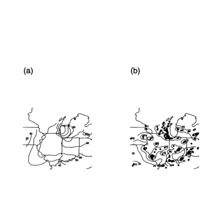
The next set of S calls evaluate the fitted surface and prediction standard errors on a grid of points. These evaluations are then converted to the format for surface plotting and some contour plots are drawn (see Figure 5).

set.panel(2,1)

predict.surface( ozone.krig)-> out.p

US( xlim= range( ozone2$lon.lat[,1]), ylim= range( ozone2$lon.lat[,2]» contour( out.p, add=T)

predict.surface.se( ozone.krig)-> out2.p

US( xlim= range( ozone2$lon.lat[,1]), ylim= range( ozone2$lon.lat[,2]» contour( out2.p,add=T)

points( ozone2$lon.lat)

The last part of this section illustrates how to extend this analysis to a covariance function that is not stationary. One simple departure from nonstationarity is to consider a covariance that has different marginal variances but isotropic correlations. Specifically consider

k(z, z')

=

u(z)u(z')eIlZ-Z/1l18

(a)

(b)

sd.tps<- tps( ozone2$lon.lat, ozone.cor$sd, return.matrices=F)

The return.matrices switch has been set to false so that the large matrices needed to find standard errors are not included in the output object. We do not need to calculate standard errors and using this smaller object in other functions is more efficient.

The next step is to call krig with a covariance function that uses this tps object to evaluate the marginal variances. The function exp. isocor in FUNFITS has been been written to do this, and the reader is referred to the help file for the details of its arguments. The main differences between this function and the other examples that have been given is that it needs the tps object3 passed to it in order to evaluateO'(:ll)and it also has an option to return the marginal variance at a set of locations instead of the covariance. This addition is important for predict. se to work correctly. Another difference is that this covariance builds in the nugget effect.

Here is an example of using exp. isocor based on the parameters found from the nls fitting of the correlogram. In the spirit of doing something useful with the results, the modeled covariances are compared to the observed ones (Figure6). To limit the number of points on this plot only pairs of stations within 250 miles of each other are included.

> hold1<- diag(ozone.cor$sd)y'*y'(ozone.cor$cor)y'*y' diag(ozone.cor$sd)

>upper<- col(hold1» row( hold1)

> hold1<- hold1[upper] # get upper triangle

> hold2<- exp.isocor( ozone2$lon.lat, obj=sd.tps, alpha = .93, theta=343, lon.lat=T)

> hold2<-hold2[upper]

> ind<- cgram.oz$D <= 250

> plot( hold1[ind], hold2[ind], pch='.', xlab='observed COY' , ylab='fitted COY' )

> abline(O,1)

To use krig to fit the surface one has two options. The first is to keep all of the covariance parameters fixed using the values estimated from the correlogram. Here is how to specify this model.

> weights<- 1/exp.isocor(ozone2$lon.lat, obj=sd.tps, alpha=.93, theta=343,

+ marginal =T) # reciprocal marginal variances at the observed locations

> fit.fixed<- krig( ozone2$lon.lat[good,], y16[good],

+ rho=.93, sigma2= (1-.93), weights=weights[good], + cov.function=exp.isocor,obj='sd.tps', theta=343)

The values for rho, sigma and weights are set so that the covariance agrees with the nonstationary model given above. In krig the name of the tps object is passed to the covariance function as a character string to save storage.4

The second approach is to estimate the parameters p and 0'from the data. The S code

below is for finding both parameters using GCV.

30r a character string with thetpsobject's name

4The disadvantage is that subsequent computing withfit. fixedmust also have the objectsd. tpsin

o

o

LO

o

o

-0>('1) 0>0

~u

o

o

C\I

o

o

,...

o

200

observed COV

400

'

..

600

> fit.GCV<- krig( ozone2$lon.lat[good,J, y16[goodJ,

+ weights=weights[good] ,

+ cov.function=exp.isocor,obj='sd.tps', theta=343)

This gives a very different fit to the data, and possibly reflects the fact that for this given day the ozone surface has more variability than on average. To compare the effect on the estimated prediction error using these two models, one can compare the standard errors.

> set.panel(2,2)

> out1.p <- predict.surface.se(fit.fixed)

> out2.p <- predict.surface.se(fit.GCV)

> contour(out1.p)

> contour(out2.p)

> out3.p<- out2.p

> out3.p<- out2.p$z/out1.p$z #relative difference between the SE's

> contour(out3.p)

A compromise between these two models is to specify the ratio of "noise to signal",

0'2/P= A and let0'be determined by estimates based on the data at day 16. The net result

is a covariance model where the average covariances are scaled by these two parameters.

fit.lambda<- krig( ozone2$lon.lat[good,J, y16[goodJ, lambda=(1-.93)/.93,

weights=weights[goodJ,

cov.function=exp.isocor,obj='sd.tps', theta=343)

out4.p<- predict.surface.se( fit.lambda) contour( out4.p)

6

Generalized ridge regression

Both the thin plate spline and the spatial process estimators have a common form as ridge regressions. This general form is at the heart of the numerical procedures for both methods so it is appropriate to outline it in this overview. Assume the model

Y =Xw+e

and suppose that H is a nonnegative definite.

The general form of the penalized (and weighted) least squares problem is minimize

(Y - XwfW(Y - Xw)

+

AWT Hw

over wE1RN

The solution is

(4)

w

=

(XTWX

+

AH)-lXTWY

The details of the computation are given at the end of this section. Given this general framework, the specific applications to thin plate splines and spatial process estimates in-volve identifying the relevant parameterization to get the X matrix and the penalty matrix,

•

Consider a function estimate of the form:

t N

f(a:) =

L

c/>j(a:).Bj

+

L

?Pi (a:)6i

j=l i=l

where {?Pi} are a set ofN basis functions and c/> are t low order polynomial functions5 _For

both thin plate splines and the spatial process estimates, the parameter vectors 6 and.Bare

found by minimizing

(Y - T.B - M6fW(Y - T.B - M6)

+

>'6Tn6

Here>.

>

0,

n

is a nonnegative definite matrix, Tk,j

=

c/>j(a:k), Mk,i

=

?Pi(a:k), and W

is a diagonal matrix proportional to the reciprocal variances of the errors. By stacking the parameter vectors and augmenting the penalty matrix with zero blocks this problem can be written in the same form as a general ridge regression. One important detail of this

correspondence is that when a basis function is defined for each unique a: (e.g n = N),

6 must satisfy the linear constraints

rT

6

=

O. The discussion at the end of this section

explains how this constraint is enforced by reparametrizing to a reduced model.

Note that the penalty or ridge term does not apply to the parameters of the polynomial part of the model and this division corresponds to the fixed part of the spatial model or the

null space for a thin plate spline. Usually

n

is constructed so that the quadratic form6T_n6

measures the roughness of the function. However, in connection with kriging estimators,

n

is the covariance matrix of the random surface.

6.1

Details of

tps

and krig

Given the ridge regression structure of the estimates, it is sufficient to describe the particular basis functions associated with each estimate and how the independent variables are scaled.

Let {a:i} for 1 ~ k ~ N denote a set of knots. In most cases the knot sequence will be

equal to the unique set ofa: values but the only real restriction is that N ~ n. Here we are

using the knot terminology loosely since these are really join points of the function only in the case of thin-plate splines in one dimension. For higher dimensions the knots specify the location of the basis functions.

Fortps let ?Pi (a:) = Emd(a: - a:i) where Emd are the radial basis functions

Emd(r)

=

amd

II

r 1I(2m-d)log(1I r

II)

=

amd

II

r 1I(2m-d)

d even

dodd

andamd is a constant.

The inclusion of the log term may seem mysterious but is necessary for even dimensions. Without this nonlinear term, the basis functions would be the norm raised to an even power and thus would add together to give a single low order polynomial. Before performing the thin-plate spline calculations, the default is to scale each dependent variable to have unit standard deviation. This operation assumes that on a standard scale the function has approximately the same smoothness in each dimension. Other scaling options are also supported. Although a more intensive approach is to estimate a separate smoothing scale for each variable by GCV (Gu 1991), this extension has not been implemented in FUNFITS because of the additional computational burden.

..

The roughness penalty matrix for thin plate splines reduces to the simple form:

Hk,j

=

tPk(Zj)

=

Emd(zj - zk)

and a derivation may be found in Wahba (1990). In approaching this theory the reader

should keep in mind that although a Hilbert Space development simplifies the notation and is elegant, the basic tool to justify this formula is a multidimensional integration by parts formula. One point of confusion in regard to this form of the roughness penalty is that it

is only correct if some specific linear constraints are placed on

o.

However these constraints

arise naturally in restricting the number of parameters when one takes a knot at all unique

values ofZk. In one dimension these constraints are the natural spline boundary conditions

whereby the estimate is forced to be linear beyond the boundary knots.

For the krig function let tPk(Z) = k(z,z;). Because the covariance function should

include the natural scaling of the variables as part of the range parameters, the default for

krigis notto do any scaling of the variables. The roughness penalty matrix for the spatial

process model is

Hj,k

=

tPk(Zj)

=

k(zj, Zk)

The estimates for ..\ , (1'2 and p can be computed using the general form of the ridge

regression problem and by default these are found using GCV and sums of squares of the residuals and predicted values. An alternative approach is to estimate these parameters by restricted maximum likelihood under the assumption of a Gaussian field (O'Connell and Wolfinger, 1996).

6.2

Computation of the ridge regression estimator

This section discusses the details of computing the ridge estimates and concludes with a discussion of the merits of this computational approach over previous work.

Recall the generic quadratic minimization problem for both the spline and spatial process

estimates in equation 4. Taking partial derivatives with respect to 0and j3 and simplifying

gives the following system of equations that characterize the minimizer.

-MTW(y - Tj3 - Mo)

+

..\00

-TTW(y - Tj3 - Mo)

o

o

(5)

In the case thatM

=

0 and has full rank, with some substitutions these may be simplified to

WTj3

+

(..\I

+

WO)O

=

TT O

Wy

o

(6)

This latter case is the usual form for the thin plate spline and kriging estimators and the standard way of solving this special case is discussed in Bates et al. (1987). The Bates et

al. (1987) solution is implemented in the FUNFITS functiontpsregbut the simplification

is not used for the general case when M is not equal to O. To enforce the constraint on

o

implied by the second equation, let T = FiR denote the QR decomposition of T where

F

=

[Fi

I

F2] is an orthogonal matrix, Fi has columns that span the column space ofT

and R is upper triangular. Reparametrizing by 0= F2W2 for W2 E~n-t now enforces the

We now write the general minimization problem in ridge regression form. Let, {3

==

Wl and wT

=

(Wl,W2)T. The following linear system ofn equations now describes the minimization:

xTwxw +>'Hw = XTWY

where

H =

(~ Fi~F2)

and X

=

[T

I

M F2] Clearly, once w is found this can be translated back into the original

({3,8) parameterization.

The computational approach for solving this system is based on the need to find w

over many values of

>..

Also there is an interest keeping the numerical strategy simple so

the source code is accessible to others. Let B denote the inverse symmetric square root

ofXTWX. Currently B is constructed from the singular value decomposition ofXTWX

but a Cholesky square root is equally reasonable. Now let UDUT be the singular value

decomposition of BHB and set G

=

BU. With these decompositions and notation the

system of ridge regression equations is

B-l(I

+

>.BHB)B-1w B-1(I

+

>.UDUT)B-1w B-1U(I

+

>.D)UT B-1w

giving the solution

(7)

Note that the matrix inverse is conveniently evaluated because it is diagonal.

This numerical approach is closely related to constructing a Demmler-Reinsch basis for

the smoothing problem. This basis is denoted by {gv} and is defined by the three following

properties.

1. {gv} for 1~ v ~ N spans the same subspace as {<Pi},{1/;i}

2. Lkg~(:l:k)Wkgv(:l:k)= 8~,v where 8~,v is Kronecker's delta function.

Technically this basis is orthogonal with respect to the inner products derived from weighted residual sums of squares and the roughness penalty. Let

N

1(:1:)

=

L c¥vgv(:I:)

v=l

and assume that N = n (there are as many knots as unique:I: values). Then

n n

L(Yk - 1(:l:k))2Wk= L(uv - c¥v)2

--

and

n Jm(f) =

L:

DvCi~

v=l

where U_v = L:~=lgv(Zk)WA'yk. Based on these relationships it is easy to show that the

spline solution has the simple representation:

N

, ~ Uv

/(z) = L..J l+AD gv(z)

v=l v

Moreover, assuming the basic observational model, the random vector u has an identity

covariance matrix. Although the Demmler-Reinsch basis is not explicitly used in the tps

function is it easy to recover and the FUNFITS functionmake. drbevaluates this basis using

the output object from tps. In terms of the matrix expressions, gv(Zk)

=

(XGh,v.

Based on the decompositions outlined above, there are also simple forms for A(A), the

trace of this matrix and the GCV function

Straight forward algebra verifies that aTxTWXG = UTBXTWXBU = UTU = I and

thus

There is also a simple formula for the weighted residual sums of squares. Add and subtract

A(O)

=

XGGT XTW from A(A) and one can derive

yT(I - A(A))W(I - A(A))y

yT(I - A(O))TW(I - A(O))Y

+

yT(A(O) - A(A))TW(A(O) - A(A))Y)

SSpure

+ IIA(I +

AD)-luIl2

N

(A

)2

SSpure

+ {;

1

+

~~k

whereSSpure

=

yT(I - A(O))W(I - A(O))Y andu

=

aT XTWY.

Thus we see that the residual sums of squares can be evaluated in order N operations

for different values ofA provided that the decompositions u and SSpure have been found.

The residual sums of squares attributable to pure error, SSpure, is the result of the

weighted regression on the full basis without any smoothing. If N ~ n and there are no

replicated points then this is zero. However, in the presence of replicated observations this will be the usual sums squares based on (weighted) differences between group means and the replicated points.

The simple form of the solution in (7) is appealing but comes with some numerical

disadvantages. The most serious is that XT_{WX may not have full numerical rank and so}

constructing the inverse square root is problematic. Our experience is that a large condition

number usually occurs for one-dimensional problems (try auto.paint) or when the data

points have similar dependent values

(lIz, -

Zj

II

is small). A natural solution to this problem

•

used in FUN FITS although the problem is that once this is done one can longer interpolate the data or fit models that have a very fine resolution. For most applications involving some measurement error this is not an issue.

Another draw back is that two intensive matrix decompositions are done instead of one.

The first is computing the inverse square root ofXTWX and the second is a singular value

decomposition of a matrix related to to the roughness penalty. In the case whenM = none

can avoid the first decomposition using the thin-plate spline algorithms of Bates et al. (1987) as implemented in the FUNFITS function tpsreg. In fact, even the second decomposition can avoided by working with tridiagonal systems (Gu 1991). In either case, one must work with a complete set of basis functions and so even with this efficiency the computation of a thin plate spline is practically limited to several hundred observations (not counting replications). By contrast, the FUNFITS tps algorithm provides approximate estimates for much larger sample sizes and is particularly efficient when one expects a moderate random component in the model. This is the case when the number of knots is much smaller than the number of observations.

7

Fitting single hidden layer neural networks

The form of the feedfoward single layer neural network is

M

f(z)

=

f30

+

'Ef3k¢(J1.k

+

If

z) k:l

where ¢(u)= (etl_)j(l

+

etl

) is the logistic distribution function. The parameter vectors are

f3, Pk and Ik , 1~k ~ M giving a total number of parameters equal to 1

+

M

+

M

+

dM =

1+M(d+2).These parameters are estimated by nonlinear least squares and the complexity

of the model, i.e. the number of hidden units M, is chosen based on generalized

cross-validation: GCV(p)= RSS(p)j(l- Cpjn)2. The usual procedure is to fit a range of hidden

units, for example one to five, and choose the model with the minimum value of the GCV function. This is the default model as saved in the nnreg object. We prefer a cost value,

C= 2, to guard against the over fitting that is inherent with neural network representations.

7.1

Details on fitting the model

The parameter space has a very large number of local minima when nonlinear least squares is used to estimate the neural net parameters. Thus, a conservative computational strat-egy is to generate many parameter sets at random and use these as starting values for the minimization procedure. To make this search procedure clear, we refer to the default num-bers and argument names from the nnreg function. Minimization of the residual sums of

squares is done independently for each value ofM. A rectangular region offeasible

param-eter values (with respect to the properties of the logistic function) is divided into a series of 250 (ngrind) nested boxes about the origin. For each box, 100 (ntry) parameter sets are generated at random from a uniform distribution. The parameter set with the lowest RMSE is used as the initial point in the iterative minimization of the RMSE and we refer to

the results of these 250 (ngrind) trial fits as grinds. The best 20 (npolish) of these grinds,

based on RMSE, are then used for a more refined minimization with a much smaller

.

-

•

polished parameter set with the smallest RMSE is taken to be the least squares solution. The nnreg function also returns the other polished models for examination.

The care in searching the parameter space reflects our experience with the pathologies of the neural network sum of squares surface and is necessary for reproducible results. Because this fitting procedure may be computationally intensive, the nnreg function does most of its computation outside of S-PLUS. The nnreg function sets up some input files, executes a stand alone FORTRAN program in the UNIX shell and then reads in an output file when the program is done. This structure has the advantage that the fitting procedure can be run in the background independently of an S-PLUS session and the nnreg function has switches to set up the input file or read in the output file independently of executing the program. This may seem like a throwback to FORTRAN programming days, but for this application it seems appropriate. Along these lines the print function for the nnreg object lists the summary output file from the FORTRAN program.

Another point of possible confusion is the form of the logistic function (the squasher function) used by nnreg. The exponential form has been approximated by a rational poly-nomial. This approximate form (see nnreg. squasher) does not change the approximation properties of the neural network and is much faster to evaluate.

7.2

Confidence sets for the model parameters

The construction of confidence intervals for the neural net regression estimates is based on the identification of a joint confidence region for the model parameters using the likelihood ratio statistic. To simplify notation, it is helpful to stack the parameters in a single vector, (). In this form, the approximate confidence set is all the values of () such that

S«(})

~

S(O)

[1

+

-P-F(p,

n-

p,

ex)]

n-p (8)

where S«(}) is the residual sum of squares,

0

is the least-squares estimate of (). For the F

distribution, p is the total number of parameters in the model, n is the sample size and ex

is the probability level.

By default, the nnregCI function computes a set of 500 parameter vectors which satisfy

the inequality of (8) with ex

=

.05 (95% level of confidence). Some attempt is made to

choose these representative vectors to fill out the confidence region for () and the confidence set for any function of the parameters can be approximated using these representatives. Let

If'«(}) be some functional of the neural network model that is of interest. For example, If'«(})

could be the predictions of the mean function at specific x values. A more complicated

functional is to consider the Lyapunov exponent when the neural network has been used to fit an autoregressive time series model. The confidence set (or interval) is approximated

by evaluating If' at all the representative parameter vectors found by nnregCI. When If'is

univariate, a reasonable simplification of the confidence set is to report the interval given by the minimum and maximum of these values. An example of the nnregCI function will be included in the next section as an application of confidence intervals for Lyanpuov exponents.

8

Nonlinear Autoregressive Models

•

where

f

is a smooth function, {St} a sequence of covariates and {et} are mean zero

inde-pendent random variables. The obvious approach is to consider this time series model as a regression problem. Once a suitable "X" matrix has been created involving the lagged Y series and the covariates, this can be passed to the regression functions. The function nlar (and object class) is a convenient function that accomplishes these manipulations. To make these operations explicit, an example for fitting a model to a times series from the Rossler system (rossler) follows. The user should keep in mind that this example is given for exposition of the methods. The nlar function while more of a "black box" gives the same analysis with fewer steps. For the Rossler time series, the present value is modeled as

a function of the past three lags and

f

is estimated using a neural network model with 4

hidden units. The plots from this example are given in Figure 7.

> rossler.xy <- make.lags(rossler.c(1.2.3»

> rossler.nnreg <- nnreg(rossler.xy$x. rossler.xy$y. 1. 4) # this takes awhile

> plot(rossler.nnreg)

> acf(rossler.nnreg$residuals) # plot autocorrelation function of the

# residuals

8.1

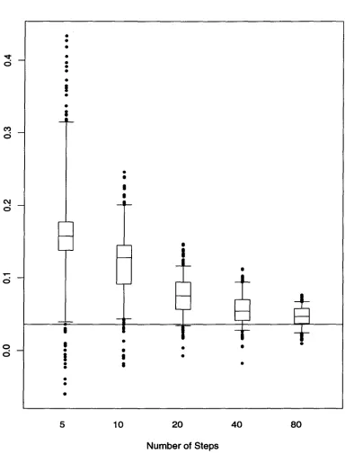
Lyapunov exponents

A typical analysis of a nonlinear system includes examination of the local and global Lya-punov exponents (Bailey et al. 1996). Based on a first order Taylor series, these quantities measure the effect of a small perturbation on the state of the system a specific number of

time steps into the future. The FUNFITS function llecalculates these statistics from the

partial derivatives of the estimated function,!. For the Rossler example:

> rossler.jac <- predict(rossler.nnreg. dervative=1)

> rossler.lle <- lle(rossler.jac)

> summary(rossler.lle)

estimated global exponent 0.03516533 summary of QR estimate

R mean Std.Dev. Q1 median Q3

5 steps 393 0.164280 0.073891 0.138140 0.157240 0.176960 10 steps 388 0.121440 0.045294 0.091214 0.127710 0.144920 20 steps 378 0.076239 0.026980 0.066031 0.074700 0.093949 40 steps 358 0.066560 0.020770 0.040733 0.063489 0.069473 80 steps 318 0.046032 0.013269 0.036481 0.046988 0.067106

> plot(rossler.lle)

.

-nlar(Y

= rossler, lags = c(1, 2, 3), k1 = 1, k2 = 4)

.-.

-R**2 =99.84% RMSE=0.3186

•

10

_•

•

--

•

••

•

•

•

Il)

..

•

•

0 _c:i

--10 rn

a; 0

:::::l

>-

"0 _c:i

0 °Cii

CD

r-IO

•

I Il)

_•

c:iI

_•

•

• • •

•

••

_•

•

_•

-

•

10 _q

•

--

I

...

I

-15 -5 0 5 10 -15 -5 0 5 10

predicted values predicted values

GCVand GCV2 Root Mean Squared Error

~

##par=:

•

0 ##units=

C"':i ~

_...

-~

N

>

0 _"!

0

c:J N

w

...

"0 en

c::: _::::i:

as

_a:

_•

-

_--

co

-

_>

C! c:i

0

...

c:J

'''It

2 c:i

•

0

•

ci

10 15 20 10 15 20

Number of Parameters Number of Parameters

'0

range of significantly positive and negative local exponents are found suggesting that in some regions of the state space the system is more sensitive to small perturbations and in other regions the system is more stable.

Finally this analysis is repeated using thenlar function:

> rossler.nlar <- nlar(rossler, lags=c(1,2,3), method="nnreg", k1=1, k2=4)

# this takes a while

> plot(rossler.nlar)

> rossler2.lle <- lle(rossler.nlar)

Note that the main job ofnlar is to keep track of the time series structure. Also the

lle function has been overloaded to use the information directly from the returned nlar object.

8.2

Confidence regions

The FUN FITS functionnnregCI will be used to calculate a 95% confidence interval for the

global Lyapunov exponent of the Rossler example. To construct a confidence interval for the global Lyapunov exponent, it is necessary to evaluate the global exponent for all 500 neural

net modelsretruend bynnregCI. The range of these values is taken to be an approximate

confidence interval for the global exponent estimate.

> rossler.Clfit <- nnregCI(rossler.nnreg) # 500 representative fits

# based on the best 4 hidden unit fit

# this takes awhile!

> hold<- rep(NA,500)

> for (i in 1:500){

# loop through all the representative parameter vectors

jac <- predict(rossler.Clfit$model[[i]],rossler.Clfit$x,derivative=1)

hold[i] <- lle(jac,nprod=NA)$glb # calculate global LE

# but not the locals

}

> rossler.le.CI <- range(hold)

The estimated global exponent is 0.035 with a 95% CI (0.017,0.036).

8.3

State vector form

Often a system is described in terms of a state vector and a map that updates this vector from the present time step into the next.

HereWt E~duniquely describes the state at timet, F :~d-+ ~dand the stochastic terms,

Et are assumed to be uncorrelated random vectors. This section ends by briefly explaining

how FUNFITS can be adapted to fit nonlinear state space models.

As an example, the usual state vector form for the Rossler system is in terms of a three

dimension vector: _Wt = _{(Xt ,}yt,Ztf. The data set rossler. state gives a realization

".

•

•

•

•

C\I

ci

•

I

•

,...

ci

o

ci

I

•

•

I

••

••

•

5

•

•

•

•

10

•

•

20

Number of Steps

•

•

40 80

-.

directly it is not difficult to fit models for each component ofF separately and combine these to estimate local Lyapunov exponents. First one needs to create the lagged set of values and fit separate (one dimensional models) for each component ofW.

> out<- make.lags(rossler.state. nlags=c(1»

> tit.ross.X<- nnreg( out$x. out$y[.1]. k1=4.k2=4)

> tit.ross.Y<- nnreg( out$x. out$y[.2]. k1=4. k2=4)

> tit.ross.Z<-nnreg( out$x. out$y[.3]. k1=4. k2=4)

Here the regression methods are neural networks fixed at 4 hidden units. However, any fitting method can be used here and the methods may be different among the different components. To find the local exponents one needs to create the Jacobian matrices for F evaluated at each state vector and pass them in the correct format to lle. In this step the important point is to string each Jacobian matrix row by row into a single long row at each time point. The resulting matrix is then the object passed to 11e.

> tempx<- predict( tit.ross.X. derivative=1)

> tempy<- predict( tit.ross.Y. derivative=1)

> tempz<- predict( tit.ross.Z. derivative=1)

> ross.jacobian<- cbind( tempx. tempy. tempz)

> ross.lle.state<- lle( ross.jacobian. statevector=T)

In this example ross. jacobian will have 9 columns and the Jacobian matrix at say the

t = 25 could be constructed by

matrix(ross.jacobian[25.]. ncol=3.byrow=T)

Those familiar with state space models will also realize that the autoregressive model based on one time series also has a (trivial) state vector form. For the Rossler example presented in the beginning of this section, letWt

=

(Yi,Yi-bYi_2)T and

Given this form, one could construct the Jacobian elements explicitly and call11e with the statevector format.

> jac<-predict( rossler.nnreg. derivative=1)

> test<- matrix( O. ncol=9.nrow=nrow(jac» # till a matrix with zeroes

> test[.1:3]<-ross.jac

>test[,4]<- 1 > test[.8]<-1 > # the rest of the elements are zero!

> ross.lle<- lle( test)

9

Model components and graphics options

The nnreg, krig, and tps functions produce fitted objects having a component best . model. For the nnreg function, this is the number of the model with the minimum GCV function value for cost=2. The best.model component for tps is the value of lambda used in the fit, and, for krig the best.model component is a vector containing the value of lambda, the estimated variance of the measurement error and the scale factor for the covariance used in the fit. The plot functions for nnreg, krig, and tps by default will use the best.model component for the summary plot.

The FUNFITS plotting functions have some intelligence in controlling the layout of

the graphs. If the plotting window has already been divided up into a panel then the

FUNFITS functions will use this layout when it produces multiple plots. To signal that the function should not alter the plotting panel parameters one uses the logical argument graphics. reset. For example the following examples will produce summary plots from two tps fits on a single page.

> ozone.tps1 <- tps(ozone$x.ozone$y) # thin plate spline fit to data

> ozone.tps2 <- tps(ozone$x.ozone$y.lambda=.1) # tps fit with lambda=.1

> set.panel(3.2) # sets plotting array

> plot(ozone.tps1.graphics.reset=F.main=·tps fits')

# summary plot of first fit

> plot(ozone.tps2.graphics.reset=F.main=· .)

# summary plot of second fit

Besides changing the number of plots per panel, the graphics functions may also make other modifications to the default graphical parameters. For example the type of plotting region or the size of labels might be changed to produce a special plot. After the function is finished plotting there is the option of restoring the graphical parameters to their original val-ues or leaving them in their new states. This decision is also controlled by graphics. reset argument and has the default value of true, resetting the parameters to their old values. Although this is usually what one wants, it does not make it easy to add additional features to a graph produced by a FUNFITS function. Here is an example using graphics. reset=F to add the ozone station locations onto a contour plot of the fitted surface.

> surface(ozone.tps1.graphics.reset=F)