Generating a base linear referencing system for roads and highways

GENERATING A BASE LINEAR REFERENCING

SYSTEM FOR ROADS AND HIGHWAYS

Technical Report

North Carolina Department of Transportation

June, 2000

by

William Rasdorf

Angella Janisch

Acknowledgements

TABLE OF CONTENTS

LIST OF TABLES

LIST OF FIGURES

1.0

Introduction

1.4 Case Studies 1.5 Research Approach

1.6 Context and Study Justification 1.7 Database Presentation Format

2.0

The Role of Tools

2.1 Spatial and Non-Spatial Data 2.2 Data Interoperability

2.3 Integration Inhibitors 2.4 Software Inhibitors

3.0

Referencing Systems

3.1 Topology, Geometry, and Attributes 3.2 Generic Link Node System Definition 3.3 Posted Route System Definition 3.4 Mile Post System Definition

3.5 Linear Referencing System Definition 3.6 Linear Referencing System Concepts 3.7 Referencing System Adoption

3.8 LRS IDs

4.0

System Architecture

5.0

Database Schema

5.1 PMU Link Node Referencing System

5.1.1 Link Node Spatial Topology Tables 5.1.2 Link Node Non-Spatial Attribute Table 5.1.3 Observations on the PMU Tables

5.2 LRS Implementation Example

5.2.1 LRS Spatial Data

5.2.2 LRS Non-Spatial Attribute Data 5.2.3 Other Tables

5.3 Study Goals

5.4 Study Generalizability

6.0

General Constraint and Database Table(s) for LRS Algorithms

7.0

Primary Route Algorithms for generating LRS IDs

7.2 Manual Algorithm

7.2.1 Manual Algorithm Constraint

7.3 Matching Posted Route Algorithm

7.3.1 Matching Posted Route Algorithm Constraint

7.4 Longest Posted Route Algorithm

7.4.1 Longest Posted Route Algorithm Constraint

7.5 Long Route Algorithm

7.5.1 Long Route Algorithm Constraint

7.6 Longest Route Algorithm

8.0

Secondary Route Algorithms for generating LRS IDs

8.2 Manual Algorithm

8.2.1 Manual Algorithm Constraint

8.3 Matching County Posted Route Algorithm – Stop at County Boundary and New Route

8.3.1 Matching Posted Route Algorithm Constraint

8.4 Matching State Posted Route Algorithm – No Stop at County Boundary and New Route

8.4.1 Matching Posted Route Algorithm Constraint

8.5 Long County Route Algorithm – Stop Only at County Boundary

8.5.1 Long County Route Algorithm Constraint

8.6 Long State Route Algorithm – No Stopping at County Boundary

8.6.1 Long State Route Algorithm Constraint

8.7 Longest County/State Route Algorithm

9.0

Algorithm Comparison

9.1 Quality Measures for LRS Routes

9.1.1 Length of LRS Routes 9.1.2 Number of LRS Routes 9.1.3 Processing Time 9.1.4 Other Measures

9.2 Quality Measure Results

9.2.1 Length of LRS Routes 9.2.2 Number of LRS Routes 9.2.3 Processing Time 9.2.4 Other Measures

9.3 Evaluation Outcome and Analysis

9.3.1 Primary Route Algorithm Outcome and Evaluation

10.0

Conclusions and Recommendations

10.2 Transition and Correlation 10.3 Additional Testing

10.4 Gap Roads

10.5 Errors in Database 10.6 LRS Mileposts

11.0

References

Appendix A.0 – New Hanover & Pender Road Maps

Appendix B.0 – Resulting LRS Road Maps

Appendix C.0 – Links Sample Data

Appendix D.0 – Chains Sample Data

Appendix E.0 – Locator Sample Data

Appendix F.0 – Primary Matching Posted Route Algorithm

F.2 Procedure DoPrimary

F.3 Posted Route Traversal Procedures F.4 Function CrossCB

Appendix G.0 – Primary Longest Posted Route Algorithm

G.2 Main Program

G.3 Procedure SumLength G.4 Procedure UpdateLRS G.5 Procedure ChainTraversal

G.6 Posted Route Traversal Procedures G.7 Function CrossCB

Appendix H.0 – Primary Long Route Algorithm

H.2 Procedure GrabStartLink H.3 Procedure FindConectedLink

Appendix I.0 – Primary Matching County Route Algorithm

I.2 Procedure DoSecondary

Appendix J.0 – Secondary Matching State Route Algorithm

J.2 Procedure DoSecondary

J.3 Posted Route Traversal Procedures J.4 Function CrossCB

Appendix K.0 – Secondary Longest County Route Algorithm

K.2 Procedure GrabStartLink K.3 Procedure FindConectedLink

Appendix L.0 – Secondary Longest State Route Algorithm

L.2 Procedure GrabStartLink L.3 Procedure FindConectedLink

Appendix M.0 – LRS/Link Node Figures

LIST OF TABLES

Table 3.1 Link Node System Table 3.2 Posted Route System Table 3.3 Milepost System Table 3.4 LRS System Table 3.5 Linear Locations Table 3.6 Point Locations Table 3.7 Intersections Table 5.1 Chains Table Table 5.2 Links Table Table 5.3 Locator Table Table 5.4 LRS Table Table 5.5 Places Table Table 5.6 Intersections Table Table 5.7 County Boundaries Table Table 5.8 Posted Routes Table Table 5.9 Railroad Crossings Table Table 5.10 Posted Route Classifier Table Table 5.11 Pavement Condition Table Table 5.12 Node Coordinates Table Table 5.13 Route Type Table Table 5.14 Counties Table Table 5.15 Urban Areas Table Table 5.16 C & U Areas Table Table 6.1 LRSChains Table

Table 7.1 Primary Algorithm Constraints Table 8.1 Secondary Algorithm Constraints

LIST OF FIGURES

Figure 3.1 Link Node System Figure 3.2 Posted Route System Figure 3.3 Milepost System Figure 3.4 LRS System

Figure 4.1 Overall System Architecture

Figure 5.1 Route Generation System Architecture Figure 7.1 Primary Posted Route Chain Traversal

Figure 7.2 LRS Configuration for Matching Posted Route Algorithm Figure 7.3 LRS Configuration for Longest Posted Route Algorithm Figure 7.4 LRS Configuration for Long Route Algorithm

Figure 8.1 The Fork Problem

Figure 8.2 Secondary Posted Route Chain Traversal

Figure 8.3 LRS Configuration for Matching County Posted Route Algorithm Figure 8.4 LRS Configuration for Matching State Posted Route Algorithm Figure 8.5 LRS Configuration for Long County Route Algorithm

Figure 8.6 LRS Configuration for Long State Route Algorithm Figure 9.1A Primary – Matching Posted Route Algorithm Lengths

Figure 9.1B Primary – Matching Posted Route Algorithm Average Lengths Figure 9.2A Primary – Longest Posted Route Algorithm Lengths

Figure 9.2B Primary – Longest Posted Route Algorithm Average Lengths Figure 9.3A Primary – Long Route Algorithm Lengths

Figure 9.3B Primary – Long Route Algorithm Average Lengths

Figure 9.4A Secondary – Matching County Posted Route Algorithm Lengths Figure 9.4B Secondary – Matching County Posted Route Algorithm

Average Lengths

Figure 9.5A Secondary – Matching State Posted Route Algorithm Lengths

Figure 9.5B Secondary – Matching State Posted Route Algorithm Average Lengths Figure 9.6A Secondary – Long County Route Algorithm Lengths

Figure 9.6B Secondary – Long County Route Algorithm Average Lengths Figure 9.7A Secondary – Long State Route Algorithm Lengths

Figure 9.7B Secondary – Long State Route Algorithm Average Lengths

1.0

Introduction

The need to share information both within and outside transportation agencies is rapidly increasing. As this need increases, the need to maintain road and highway information in a homogeneous manner also increases.

One of the many problems associated with maintaining highway and road information is the lack of a unique way to reference a particular road or section of road. That is, how do we uniquely name a place on a roadway? Or given the node of a place, how do we exactly know where that place is? This problem arises because of the lack of permanent, fixed street and road naming standards. Although using “real-world” names as a means of referencing roadways within an organization may be acceptable, problems occur as names change over time and as non-unique names arise once agencies go outside of the organization and into different jurisdictions [Butler 1996].

This indicates a need for a standardized location referencing system (LRS), that is, a means of accurately describing the location of a physical entity. A linear location referencing system (LLRS) is a means of describing a physical location on a linear network. This is the type of location referencing system most useful in transportation, as the highway system is a linear network [Adams 1995]. The acronym LRS is used herein to encompass both LRS and LLRS.

A linear referencing system utilizes an LRS ID, which is simply a unique individual identification number for roadways that can be used for identification or naming purposes. This identifier would be used in much the same way that a social security number is used for unique identification.

The intent of this study was to explore different referencing systems, their definitions, and the information structures associated with each, as well as to clearly state the study goals. Alternative methods for generating a Linear Referencing System are also presented as well as the constraints imposed on the various methods. The different methods are then compared and the best LRS system is recommended.

1.1 Background

Departments of Transportation (DOTs) collect and store vast amounts of data. Surveys are conducted to gauge accident-prone intersections, pavement conditions, traffic load, etc. Although each individual survey is conducted for a specific purpose, all have a common thread – location.

The primary goal, when referring to transportation data, is to relate that data back to a specific place. Since all survey data share location as a common thread, the way in which different departments refer to specific locations should be the same. Quite often, each department within DOTs collects and stores locational data differently. This results in significant amounts of money and man-hours being spent on redundant efforts for collecting and storing such information [Rasorf 2000, Rasdorf A1999].

To minimize or eliminate these redundant efforts, DOTs must organize a system that all departments may use to refer to locational data. This paper describes such a system and refers to it as a Linear Referencing System (LRS). An LRS is an approach used to refer to location. Once an agreed upon LRS is accepted as a standard, all departments may use this information to refer to specific places within the roadway network.

1.2 The Purpose of the Study

This study introduces and describes both the link node system and the linear referencing system. It briefly mentions several other referencing systems as well. The purpose of the study is to explore and define several different algorithms, which can be used to generate a linear referencing system based on a preexisting link node system.

That is, we devised a set of algorithms that use as input a network of data currently stored in a link node format. The algorithms generate as output that same network of data, but this time in an LRS format. This study then compares and evaluates each algorithm against a set of predefined criteria that measure their quality or desirability of the different outcomes of each algorithm. The objective of the work is to provide DOT with a picture of what the ideal (for NC DOT) LRS might look like, for various alternative configurations, and to provide a set of measures for each configuration, thus, enabling DOT to select a suitable one for permanent implementation.

1.3 Goals

This study explores several different LRS configuration algorithms. Each algorithm explores various constraints and how they affect the final outcome. After evaluating the outcome of the algorithms, we recommend a strategy for evaluating the design and implementation of a Linear Referencing System, provide measures for impact (based on the testing of various criteria), and recommend implementation tools (such as a geographic Information System (GIS), database, or other tools and environments) and strategies.

1.4 Case Studies

roughly 195,000 for the entire state to about 1,200 for Pender County and about 2,500 for New Hanover. Both data sets contain primary and secondary roads. The smaller sample sets allow for faster processing, ease of checking the preliminary designs, and ease of evaluation of the results.

It should be noted that it is not yet possible to execute an algorithm on a statewide basis for two reasons. First, the data sets for each county’s data are presently being “cleaned” and are not in a state that the algorithms could operate on them successfully. What this means is that the database contains errors that would not permit the algorithms to run properly. Second, even if the first problem were solved, there are still county-to-county data inconsistencies that need to be resolved that would also effectively disable the algorithm. However, this cleanup is underway and two very high quality data sets are emerging: a tabular file containing accurate attribute data and a CAD file containing accurate graphics and linework for the roadway network.

Using these files, and the algorithm developed as a result of the work reported herein, will enable NCDOT to generate its permanent base LRS and standardize all state locational data. This standard will then be adopted for the development of all new data sets. Legacy data sets will either migrate to the new data standard or utilize conversion routines to translate between the two.

North Carolina’s Department of Transportation provided the GIS road coverage and Oracle database tables for Pender and New Hanover County, as well as the attributes associated with the file. The files provided are 95% error free. This represents a measure, meaning that the data have already been “cleaned” as noted above.

1.5 Research Approach

The overall goal of the NCDOT is produce and implement a fully functional linear referencing system, which can be used by a variety of its internal organizational units. The goal of this study is to identify and name the LRS routes comprising that LRS network. However, for this to happen, a research approach had to be developed and a sequence of activities had to be defined and completed.

The first of these activities involved a clear definition and understanding of the existing link node system. An understanding of the problems and limitations associated with such a system was crucial in order to achieve effective problem definition and identification. A link node a data set was acquired from North Carolina’s DOT for New Hanover and Pender counties. This provided a clear picture of the existing data and it’s link node format.

measures was developed and each algorithm was assessed based on these measures. The “best” algorithm was chosen and recommended for implementation.

1.6 Context and Study Justification

As noted earlier, the context of this study is two of North Carolina’s 100 counties. Although this is a small number of counties, the number of records for these two counties is significant enough to generate interpretable results. This is even truer in light of the fact that some very computationally intensive algorithms are used to process this data. In order to run multiple tests with a number of algorithms and get results in a reasonable time frame, we limited the test case size. However, when the study is complete, when the factors affecting the algorithm have been evaluated, and when the final algorithm has been selected, designed, and coded the context will be expanded from the test case to all 100 counties.

1.7 Database Presentation Format

This report uses a relational database schema for representing the data. The schema in is designed to work with the data as it currently exits and as it incorporates the proposed linear referencing system.

The format of the proposed design is presented in two ways. One way is purely textual and is achieved by identifying the table name along with the primary key(s) and attributes in an enumerated fashion, as follows:

TABLE NAME (Primary Key, Attribute 1, Attribute 2, Attribute 3, …, Attribute n)

Another way is tabular in which the column headings identify the type of data in that column and the rows contain the actual data. Both of these representations are used herein.

Table # – TABLENAME

2.0 The Role of Tools

Geographic Information Systems (GISs) have emerged as useful and powerful tools for storing and using spatial data. They incorporate capabilities that enhance one’s ability to perform complex spatial analysis over some geographic region. Database management systems also have emerged as useful and powerful tools. They store what we refer to as tabular data, or data that describes that attributes and characteristics of other data or of physical objects.

2.1 Spatial and Non-Spatial Data

Both of these tools are finding ever increasing uses in Departments of Transportation (DOTs) and other transportation and infrastructure areas and applications, and rightly so [Primer 1994, Butler 1996]. They support improved performance of engineering systems by providing new and unique views of those systems through the spatial and attribute data that describe them. But historically GISs have been used primarily for spatial analysis and databases, or files, have been used primarily for data analysis.

Fortunately, the spatial and tabular data worlds are coming closer and closer together. GISs support some limited tabular data management and analysis capabilities. Some Database Management Systems (DBMSs) support limited spatial data management and analysis capabilities. But for large production oriented transportation and infrastructure applications, each tool needs to be used in such a way that its strength is maximized. Quite frankly, neither tool can do the other’s job very well. Thus the ultimate optimal use of these tools is in unison, in an integrated environment, where each uses the same underlying data set to do the type of work it does best.

2.2 Data Interoperability

In a traditional setting, the most common scenario has been that production programs use large data sets without making use of a geographical analysis and display capability. Likewise, GIS departments initially focus on maps and spatial representation development and often do not access engineering attribute data. This is a reality and it must simply be recognized and accounted for or system improvements will not be forthcoming.

What is desired is a way to develop, manage, and maintain data sets that can be used by both GISs and by application programs and can be moved between them with ease. Furthermore, the data sets must be designed in such a way that spatial data is inherently contained within them regardless of whether they reside in the GIS, the DBMS, or elsewhere [NCHRP 1998]. Such data interoperability is a key objective for the NC DOT.

2.3 Integration Inhibitors

seamless GIS/DBMS integration and, most often, there wasn’t even a concept of the need to share the data they contained. Thus, localized decisions were made regarding the spatial referencing system associated with the data. The result is that legacy systems have widely varying spatial referencing systems that actually inhibit data exchange.

Another problem in achieving seamless integration is that GIS and DBMS tools themselves have not historically been integrated. These products have been highly successful commercially as stand-alone products just like many engineering software products. Customers have been so happy to gain the productivity enhancement offered by popular programs (MicroStation for drafting, Oracle for DBMS, etc.) that they were satisfied with stand-alone operation. However, as that became the norm, and as their competitors come up to speed with similar software, customers began seeking a new computing productivity enhancement – integration.

2.4 Software Inhibitors

Integration also is particularly useful where an apparently stand-alone software program turns out to less stand-alone than originally thought. Consider CAD, for example. Its purpose has largely been to automate the process of creating complex sets of architectural and engineering drawings. It has fully met this need and many of the other software products have done the same.

However, some software is limited in its usefulness, although that may not be apparent initially. GIS software is turning out to be such software. GIS software is much like CAD in that it has great value as a presentation tool. Unfortunately, because presentation is not really its purpose, users have discovered that the true utility and value of GIS comes from attaching data to the geographic entities represented by GIS [Miles 1999]. Yet GISs strength lies in its spatial representation and spatial analysis, not in its ability to store and process data.

3.0 Referencing Systems

Location referencing systems may include geodetic or geographic points of reference. A geodetic referencing system defines placement on the earth’s sphere with latitude, longitude and elevation. A geographic referencing system uses planar coordinates to define a location on the earth’s surface.

Transportation poses a unique problem with respect to spatial representations and location [Adams 1995]. In the case of a state roadway network, for example, the focus of interest is on the linear nature of the network. Location is defined with respect to the lines of the network. Thus, the term linear referencing system is applicable. Furthermore, any interest in points is usually with respect to points on or close to the lines. Thus, the focus is on only a very limited portion of the overall planar space. It is this distinction that differentiates general GIS applications from GIS-Transportation applications.

The idea of linear referencing systems is not new. In fact, many linear and location referencing systems and models exists; among them are the county/route/milepost referencing system, intersection offsets, street addresses, link node system, and linear referencing system. This study focuses mainly on two – link node and linear referencing system (LRS). A brief description of each is provided and will be discussed in this section. Some fundamental principles will be presented as well. For additional details the reader is referred to any number of authors who have documented LRSs including [Dueker 1996], [Vonderohe 1995], and [Kiel 1999].

3.1 Topology, Geometry, and Attributes

A Referencing System is made up of three distinct parts: topology, geometry, and attributes [Rasdorf D1999]. Topology describes the connectivity of the components of the system and geometry describes the precise location in space of the components of the system. Taken together topology and geometry describe the spatial aspect of a component. In most cases that spatial aspect is location or position, but it may also be a measurement such as length or distance as well.

Attribute information, on the other hand, is descriptive information. For example, pavement condition, number of lanes, etc., are used to describe the characteristics of a particular link or segment of a link. The following sections will provide some specific terminology associated with topological, geometric, and attribute information.

3.2 Generic Link Node System Definition

link is defined as arc that connects two node points. Therefore, nodes are connected through a series of links.

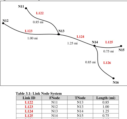
Consider an example. Figure 3.1 displays a link node topology and Table 3.1 defines that same link node topology in tabular form. Each link is provided with a unique identification number, Link ID, and is associated with its FNode and TNode. The

FNode (From Node) is a node that defines the “beginning” point of a link. The TNode

(To Node) defines the “ending” point of a link. The topology, or connectivity, is defined by matching a link’s TNode to another link’s FNode or vice versa.

Figure 3.1: Link Node System

Table 3.1: Link Node System

Link ID FNode TNode Length (mi)

L122 N11 N13 0.85

L123 N12 N13 1.00

L124 N13 N14 1.25

L125 N14 N15 0.75

L126 N14 N16 0.85

Note that Figure 3.1 and Table 3.1 inherently imply directionality. Words like from and

to imply a starting and ending point and, in the example shown, the Node ID and Link ID sequencing increases in order of FNode to TNode. But this is not a necessary constraint on the link node system. It could be that in lieu of FNode and TNode we used “node at one end” and “node at other end” as identifiers. In doing so, directionality

L123

L126 L125 L124

L122

N12

N16 N15 N14

N13 N11

1.00 mi 0.85 mi

1.25 mi

0.75 mi

becomes irrelevant and node and link numbering need not imply any sequencing or directionality. Such is the case in the NC DOT Pavement Management Unit database.

3.3 Posted Route System Definition

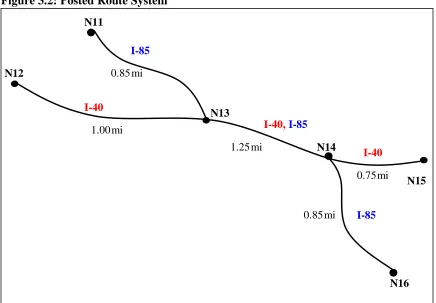
The posted route system is a naming convention widely used by state DOTs. The posted route system refers to roads and highways by the name given to links, segments of links, or multiple connected links. Its advantage is that posted route naming is used in the field on all signs and on maps and is nearly universally understood. Still, the posted route system referred to here retains the use of nodes to assist in delineation of portions of roads.

As mentioned previously, problems arise when organizations use posted route names. These problems are a result of the overlap in road naming conventions. For example, one portion of roadway may have several different posted route names (previous link 123 is now both I-40 and I-85). If one department or organization refers to this portion of roadway as I-40 and another department or organization refers to the same portion of roadway as I-85, the systems may not have the ability to combine the information gathered to form a complete analysis of the route or link. Furthermore, they may be referring to entirely different portions of I-40 and I-85. Finally, as the names of roads change over time, vital historical data may be lost.

Figure 3.2: Posted Route System

mi mi

mi

mi

0.75 I-40

I-85

I-40 I-40,I-85

I-85

N12

N16 N15 N14

N13 N11

1.00 0.85

1.25

mi

Table 3.2: Posted Route System

Posted Route FNode TNode Length (mi)

I-85 N11 N13 0.85

I-40 N12 N13 1.00

I-40 N13 N14 1.25

I-85 N13 N14 1.25

I-40 N14 N15 0.75

I-85 N14 N16 0.85

Figure 3.2 displays the posted route system and Table 3.2 defines the posted route system in tabular form. What is different here from the link node system is only that the Link ID field in the Link Node system is now replaced with a Posted Route field. All other items in the figure and table remain the same for the Posted Route system as for the Link Node system.

3.4 Milepost System Definition

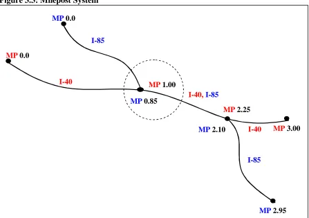
The milepost system makes use of the posted route system and simply assigns a milepost marker at each node. Figure 3.3 displays the milepost system and Table 3.3 defines the milepost system in tabular form. The milepost marker indicates a running sum of distances along a posted route or assigned LRS. MP1 stands for milepost one and indicates the first milepost marker for a given link. MP1 starts at zero at the beginning of each new posted route. It also starts at zero at each county boundary. MP2 stands for milepost two and denotes the distance to some other location along the roadway such as an intersection.

Figure 3.3 obviously differs from Figures 3.1 and 3.2 in the way the nodes are labeled. Instead of being assigned a node number, the nodes are assigned a milepost marker. Note that at some nodes more than one milepost is shown. For example, the node inside the circle has mileposts MP 0.85 and MP 1.00. This indicates that two different posted routes share the node. Posted route 85 has a milepost of 0.85 miles and posted route I-40 has a milepost of 1.00 miles at that node.

Table 3.3 is also different from Tables 3.1 and 3.2 in an important way. The use of mileposts in Table 3.3 eliminates the need to store lengths. Lengths are now calculated rather than stored. Yet at the same time, the concept of links is still implied by the new table structure in that each row in the table mimics a link.

Figure 3.3: Milepost System

Table 3.3: Milepost System

Posted Route MP1 MP2

I-40 0.0 1.00

I-40 1.00 2.25

I-40 2.25 3.00

I-85 0.0 0.85

I-85 0.85 2.10

I-85 2.10 2.95

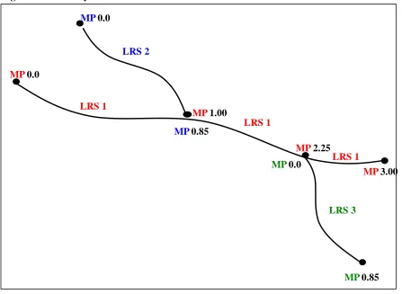
3.5 Linear Referencing System Definition

A linear referencing system is similar to the posted route system in that it groups multiple links together with the same name or ID. It is also the similar to the milepost system in that it provides each node with a milepost marker instead of a node number. However, a linear referencing system, unlike the posted route or milepost system, provides a unique and flexible way of referencing links, segments of links, and multiple links within roads and highways. Thus, an LRS provides a means for data transfer between and among organizations. It also allows for historical analysis because once a link is designated with

an LRS ID it is permanent.

I-40

I-85

I-40 I-40, I-85

I-85 MP 0.0

MP 2.10 MP 1.00

MP 2.95 MP 0.0

MP 3.00 MP 2.25

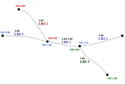
Figure 3.4 displays the LRS and Table 3.4 defines the LRS in tabular form. Any portion of road has only one identifier (LRS 1, LRS 2, LRS 3). There is no overlap of names or identification. Thus, mileage does not overlap either, except at nodes. For example, the portion of roadway on LRS 1 between MP 1.00 and MP 2.25 had no other possible MP or mileage specification. Additionally, fewer records are needed in the database to describe location as shown in Table 3.4. (Note that it is merely coincidence that LRS 2 and LRS 3 are of the same length).

Milepost markers are assigned to nodes and represent the total length of the LRS route up until that point. The total length of the LRS route is the result of the summation of the individual link lengths that comprise the LRS route. Table 3.4 provides not only the LRS ID, but also MP1 and MP2. MP1 represents an LRS Route’s very first milepost marker, which should always be 0.00. MP2 represents an LRS Route’s very last milepost marker and should always equal the sum of all the individual link lengths that comprise the LRS route.

Figure 3.4: LRS System

Table 3.4: LRS System

LRS Route MP1 MP2

LRS1 0.0 3.00

LRS2 0.0 0.85

LRS3 0.0 0.85

LRS 1

LRS 3

LRS 1 LRS 1

LRS 2 MP 0.0

MP 0.0 MP 1.00

MP 0.85 MP 0.0

MP 3.00 MP 2.25

3.6 Linear Referencing System Concepts

This section presents the most fundamental conceptual schema for implementing the spatial topology of the recommended base LRS. A centralized approach is recommended for NCDOT, but a distributed approach is also presented so that the reader can better understand the concepts and see how they represent essentially the same solution.

In the database, linear elements, such as pavement type and speed limits, are spatially defined using the base LRS. This requires a unique LRS ID for each road in the route system and a MP1 and MP2 to mark the beginning and ending locations along the specified road. Table 3.5 shows the general table structure for linear elements. Point features, such as railroad crossings, are spatially defined with the unique LRS ID and

Milepost measurement along that route as shown in Table 3.6.

Table 3.5: Linear Locations

LRS ID MP1 MP2 Any Linear Attributes

515 0.00 1.00 X

623 68.00 69.40 X

623 69.40 71.50 X

Table 3.6: Point Locations

LRS ID Milepost Any Point Attributes

623 69.20 X

624 106.20 X

Table 3.7 represents an example of the spatial topology of intersections in the LRS route system. Anywhere an LRS route crosses another LRS route an intersection occurs. The easiest way in which to identify an intersection is by using a node identifier. Thus we incorporate one of the characteristics of both the link node and posted route systems. The

Milepost field is used to represent the distance along the LRS route where the

intersection is positioned. Each intersection must be represented by at least two records containing the same Node ID. This is because there are at least two LRS routes required to form an intersection and the node will be located at a different milepost distance for each.

Nodes are not the only way that intersections can be represented in the topology. However, they do present the database with an easier query option. Information related to each intersection could be queried using the Node ID as the primary key. Nodes are separately identified because they represent a unique and distinct part of the network topology. Table 3.7 is included here to illustrate the concept of nodes and their relationship to the LRS.

Other features that interact with or intersect the roadway, such as railroad crossings, do not need to be assigned nodes because they can be located solely on the basis of the

Milepost measure shown in Table 3.6. That is, an intersection is a topological

a single road. A database designer may choose to name a railroad crossing, thus providing it with an identifier. However, that identification has nothing to do with the topology of the network. This is the key difference between the LRS and the Link Node systems. In the LRS, nodes can only be placed at intersections and represent a topological entity (intersection). In the Link Node system, nodes can be placed anywhere and represent either a topological entity or some other non-topological entity (railroad crossing). The LRS system thus demonstrates simplicity, elegance, and completeness.

Table 3.7: Intersections

LRS ID Milepost Node ID

643 32.2 N25

643 38.9 N89

745 4.7 N25

745 7.8 N89

Tables 3.5, 3.6, and 3.7 are intended to conceptually demonstrate how the spatial topology of the LRS works. In actuality there will be an assortment of non-spatial attributes linked to these spatial tables. However, the database will not always use the

LRS ID and Mileposts as keys. In some instances, other keys will be required, such as

“Station Number.” In such a case, the LRS ID and Milepost fields, while still serving as candidate keys, will also serve as attributes linked to the primary key.

3.7 Referencing System Adoption

It should be emphasized that each organizational unit may choose to use a different location referencing method in their data collection and reporting. For example, the Traffic Safety Systems Unit describes accident locations based on a distance from a particular intersection along a roadway (anchor point or intersection offset reference). They currently use parameters such as POSTED ROUTE, INTERSECTION, and DISTANCE to locate accidents.

As noted earlier, and as described in Section 3.2, the Pavement Management Unit uses a link node referencing system. Thus, there are many alternative referencing systems currently in place, in large databases, throughout NC DOT. The goal is to have these units migrate to the LRS system, replacing their current system. However, if a unit chooses not to adopt the proposed LRS in its data collection and reporting activities, then a conversion mechanism must be developed to convert a particular referencing system into the proposed LRS. These conversion mechanisms are often referred to as filters.

3.8 LRS IDs

pavement in the field. An LRS ID does not replace a posted route name, just as one’s social security number does not replace one’s name. However, it does provide a unique and efficient way of storing information in a database relative to the named pavement.

Note that in the examples provided in the previous subsections, we used two different representations for LRS Ids: a simple integer (515, 724, etc.) and an alphanumeric value (LRS 1, LRS 2, etc.). The latter is used only for presentation purposes in the text and figures of this documentation. In reality, LRS IDs are arbitrarily assigned permanent integer identifiers.

4.0 System Architecture

Currently, all relational tables of the Pavement Management Unit are stored in an Oracle database. The tables store both spatial and attribute information. (The details of the PMU database will be fully illustrated in the next section.) This PMU database information is available to other applications such as ArcInfo or Arcview, which are Geographic Information Systems (GISs) that have the ability to store non-spatial information using a relational database format. They provide a limited capability to manipulate tables and values. Since ArcInfo and Arcview are GIS software packages, they obviously allow the user to robustly display the information stored within the tables.

Tables stored in a database management system such as Oracle can seamlessly be linked to ArcInfo or ArcView with a join command through a common identifier (key attribute value) located in both the Oracle table and the ArcInfo or Arcview table. With these tools in mind, the LRS algorithms described herein are implemented in Delphi 5, which is a combination of Pascal and SQL. Delphi provides the elegant programming functionality of Pascal and the database access and manipulation capabilities of SQL The combination of Arcview and ArcInfo are used to display the roadway network and the LRS IDs. Figure 4.1 illustrates how a database management system is linked to other applications such as GIS.

Figure 4.1: Overall System Architecture

GIS

Applications

5.0 Database Schema

This section presents North Carolina Department of Transportation’s Pavement Management Unit (PMU) highway network database schema. Pavement Management currently uses the link node referencing system to store all information pertaining to the highway network. In addition to the link node system, the proposed LRS database schema is also provided. The reader is thus afforded the opportunity for a “side-by-side” comparison. Both the link node system and the LRS system have the following components: tables related to topology and geometry, tables related to attribute information, and other tables whose purpose is later explained.

5.1 PMU Link Node Referencing System

Currently the NCDOT Pavement Management Unit stores all highway/roadway information using the concept of a link node referencing system. A node point is placed at each intersection of a road. Node points are also placed at the beginning and ending points of bridges, at railroad crossings, and at county boundaries. Lines or arcs, referred to as links, connect one node to another with a line and approximate the path of the road network.

Once the links and nodes are defined, they are given a statewide unique link number (for all links) and a countywide unique node number (for all nodes). The assignment of these numbers is arbitrary, which means that no numbering pattern can presumed to be followed. The tables listed below are examples of the tables that the Pavement Management Unit uses to implement its link node system. Although the tables represent only a portion of the complete database, they are the only tables used to define the topology and geometry of the roadway network. It is from these tables that the proposed LRS algorithms originate.

5.1.1 Link Node Spatial Topology Tables

As mentioned earlier, topology describes the connectivity of a network. The following table(s) provide the structure of the topological aspects of the system. In addition to the table and the description of its attributes, Figures M.1 and M.2 from Appendix M illustrate the composition of the network.

The CHAINS table provides the topology of the roadway network by connecting each

CHAINS (Link, County, Route, Beg_MP, Prev_Link, Next_Link, MP_Node)

Link – The statewide unique link identification number given to each arc with a beginning and ending node.

County – The county the link is located in.

Route – An 8-digit number that provides information such as route classification (Interstate, US, State, or Secondary road), type of route (Business, Alternate, Regular), Direction, and Posted Route Number.

Beg_MP – Indicates the Posted Route Milepost marker at the beginning node of the link.

Prev_Link – The link number of the link directly preceding the current link. Next_Link – The link number of the link directly following the current link. MP_Node – The node number of the Beg_MP marker.

The LINKS table provides information about each individual link including its beginning

and ending nodes, the county that each is contained within, the length of each node, as well as information about whether it crosses a county boundary. The links are essentially the basic building blocks of routes.

LINKS (Link, B_Node_Cnty, B_Node, End_Node_Cnty, End_Node, Sec_Length, Gap)

Link – The statewide unique link identification number given to each arc with a beginning and ending node.

B_Node_Cnty – A number representing the county where the beginning node is located.

B_Node – A countywide unique number representing the beginning of the link. End_Node_Cnty – A number representing the county where the ending node is

located.

End_Node – A countywide unique number representing the ending of the link. Sec_Length – The length of the link (in miles).

Gap – The county that a link crosses into.

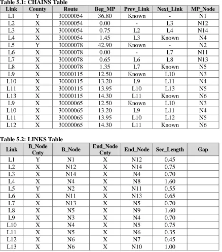
The following data tables provide a better understanding of the type of information stored in the tables defined above. The information in Table 5.1, the CHAINS table, is taken from the Link Node Figure M.1 in (Appendix M) and the Posted Routes and Posted MP Figure M.2 (in Appendix M). The information in Table 5.2, the LINKS table, is taken from the Link Node Figure M.1 (in Appendix M). Furthermore, Appendices C, D, and E each contain a subset of actual data from the PMU’s LINKS, CHAINS, and LOCATOR

tables, respectively.

Table 5.1: CHAINS Table

Link County Route Beg_MP Prev_Link Next_Link MP_Node

L1 Y 30000054 36.80 Known - N1

L2 X 30000054 0.00 - L3 N12

L3 X 30000054 0.75 L2 L4 N14

L4 X 30000054 1.45 L3 Known N4

L5 Y 30000078 42.90 Known - N2

L6 X 30000078 0.00 - L7 N11

L7 X 30000078 0.65 L6 L8 N13

L8 X 30000078 1.35 L7 Known N5

L9 X 30000115 12.50 Known L10 N3

L10 X 30000115 13.20 L9 L11 N4

L11 X 30000115 13.95 L10 L13 N5

L13 X 30000115 14.30 L11 Known N6 L9 X 30000065 12.50 Known L10 N3

L10 X 30000065 13.20 L9 L11 N4

L11 X 30000065 13.95 L10 L12 N5

L12 X 30000065 14.30 L11 Known N6

Table 5.2: LINKS Table

Link B_Node

Cnty B_Node

End_Node

Cnty End_Node Sec_Length Gap

L1 Y N1 X N12 0.45

L2 X N12 X N14 0.75

L3 X N14 X N4 0.70

L4 X N4 X N8 1.60

L5 Y N2 X N11 0.55

L6 X N11 X N13 0.65

L7 X N13 X N5 0.70

L8 X N5 X N9 1.60

L9 X N3 X N4 0.70

L10 X N4 X N5 0.75

L11 X N5 X N6 0.35

L12 X N6 X N7 0.45

L13 X N6 X N10 1.00

5.1.2 Link Node Attribute Table

Attribute data, as mentioned earlier, describes a feature or an entity. Attribute data does not provide information about the connectivity (topology) or precise location (geometry) of an item. However, attribute information is essential in providing descriptive information and is needed to make the database complete and significantly more useful.

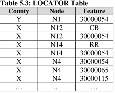
The LOCATOR table provides a description of every feature (road, bridge, etc.) at a

LOCATOR (County, Node, Feature)

County – A statewide unique number that represents the county the link is in. Node – A countywide unique number representing a roadway intersection, county

boundary, or bridge beginning or ending.

Feature – Represents every item (road, bridge, etc.) at the node; there is a separate record for each feature at a node.

Table 5.3, the LOCATOR table, provides a better understanding of the type of information stored in the table defined above. The information is taken from Figure 1B in Appendix M.

Table 5.3: LOCATOR Table County Node Feature

Y N1 30000054

X N12 CB

X N12 30000054

X N14 RR

X N14 30000054 X N4 30000054 X N4 30000065 X N4 30000115

… … …

5.1.3 Observation on the PMU Tables

Some observations about the Pavement Management Unit’s link node system implementation are in order. At first glance, one may misinterpret the B_Node and

End_Node fields in the LINKS table as denoting directionality. However, this is not the

case. As mentioned in Section 3.2, the B_Node and End_Node identifiers are assigned arbitrarily and do not provide any directional information.

Still, some general directionality can be determined through the highway naming convention adopted nationwide. This naming convention states that all posted routes with an even number generally run east and west and all posted routes with an odd number generally run north and south.

More specific direction information can be determined from the CHAINS table. This table defines all routes as a chain of multiple links. Following the links in a chain traverses a posted route. A link is listed in the CHAINS table once for each of its assigned posted routes. Therefore, a link may be listed more than once if it lies on the path of more than one posted route.

The Beg_MP provides the mile marker location for one of the nodes of the link in

The MP_Node is the node identifier where the milepost marker is posted. The

MP_Node does not necessarily match a link’s B_Node (in the LINKS table).

It should also be noted that the mile posting of all routes in the PMU link node system begins with 0 and ends with the total length of the route within a county. This is unlike the mile posting as seen on highway markers, which begins with 0.00 and ends with the total length of the posted route statewide.

In addition to providing information about the beginning point of a link, the CHAINS

table also provides the network topological information by providing information about a link’s previous and next link. The Prev_Link field is assigned a value of null at the beginning of a posted route chain. Likewise, the Next_Link field is assigned a value of null at the end of a posted route chain. The Next_Link field is assigned a value of null when a link encounters a county boundary. The Prev_Link field is assigned a value of null when the chain crosses the county boundary. Normal chain traversal occurs by following Next_Link after Next_Link until the end of the chain is reached (or

Prev_Link to the beginning). In the case of county boundaries, however, where no next

(or previous) link is identified (even though one exists), traversal can still continue. This is done simply by matching on the B_Node and End_Node of the links.

Another observation of interest regarding the PMU database lies in the county field. This field holds a numerical value (0-99) for each of the 100 counties in North Carolina. This study used county 64, New Hanover, and county 70, Pender as test cases.

The reader should further note the LOCATOR table. At first glance this would appear to be an attribute table providing attribute information about nodes. However, it is actually, subtly, a topological table. It identifies every route that passes through a node.

For example, consider Node 4 Figure M.2 in Appendix M. The LOCATOR table tells us that NC 54, NC 115, and NC 65 pass through this node. Using this information one can enter the LINKS table and search both the B-Node and the End_Node fields to find every link that touches this node (we find L3, L4, L9, and L10).

5.2 Linear Referencing System Implementation Example

This section provides examples of a set of LRS database tables. Figure M.2 in Appendix M represents a sample route system with posted routes and intersections shown. Nodes, again, are used to represent intersections, county boundaries, railroad crossings, and bridges. Figures M.1 and M.2 show the intersection and county nodes. The following tables illustrate a generic representation of how the topology and some of the attributes might be laid out in NC DOT’s ORACLE database.

5.2.1 LRS Spatial Data

terms in this section. A set of relational model database tables is presented and used to represent the spatial and geometric data of this roadway network.

All figures represent the same physical roadway networks – a simple example selected for illustration only. The example includes roadways, a county boundary, and a railroad crossing. Figure M.2 shows all of the conventional posted route information. Figure 2 shows the data for the same area in terms of the NCDOT base LRS. Finally, Figure 4 adds information to the network regarding places. Note that the data is intended more to illustrate the database design rather than to portray any actual scenario.

The following tables are used to provide the tabular data for the information shown in the figures located in Appendix M. Following these table descriptions are the actual spatial data tables that contain all the data represented in the figures located in Appendix M.

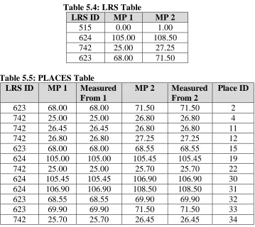
The LRS table, Table 5.4, defines the LRS routes. LRS routes are identified by each route’s LRS ID, the route’s beginning milepost (Beg_MP), and the route’s ending milepost (End_MP). Thus the route is defined in its entirety, but the definition does not include intermediate nodes or segments of the LRS route (which are defined in a separate

PLACES table).

LRS (LRS ID, Beg_MP, End_MP)

LRS ID – the statewide unique LRS identification number assigned to the road Beg_MP – the beginning LRS milepost value, which will always be 0 since it

marks the beginning milepost for each LRS route

MP 2 – the ending LRS milepost value, which will always be the LRS route’s total length

The PLACES table, Table 5.5, allows for the identification of arbitrary segments of any

road. These are identified by the road’s LRS ID, beginning milepost (MP1) and ending milepost (MP2). Thus, each table entry identifies a linear segment of roadway by establishing a relationship between places and the LRS referencing system. The Place ID is the name given to each of these roadway segments. A place may occur at any arbitrary location on the roadway network.

PLACES (LRS ID, MP1, Measured From 1, MP2, Measured From 2, Place ID)

LRS ID – the statewide unique LRS identification number assigned to the road MP 1 – the beginning LRS milepost value

Measured From 1 – The LRS milepost of the intersection/node from which the beginning milepost was measured

MP 2 – the ending LRS milepost value

Measured From 2 – the LRS milepost of the intersection/node from which the ending milepost was measured

The INTERSECTIONS table, Table 5.6, stores the nodes that represent an intersection. It gives the node identification number for each intersection, the LRS that the intersection occurs on, and the milepost it occurs at. Thus, nodes may be queried to reveal information about each intersection. Note that in the Figures in Appendix M, nodes have been placed at the ends of each route as they are drawn. These routes are actually continuous even though nodes are shown. This is only for demonstration purposes and will not occur in the actual database representation, except for roads crossing the boundaries of the State.

INTERSECTIONS (Node ID, LRS ID, LRS MP, Posted Route, PR MP, County Name)

Node ID – name/identification given to the point of intersection

LRS ID – the statewide unique LRS identification number assigned to the road LRS MP – the milepost of the intersection using LRS values

Posted Route – the name (number) of the posted route

PR MP – the posted milepost of intersection on the posted route County Name – the county in which the intersection is located

The COUNTY BOUNDARIES table, Table 5.7, stores the nodes that represent county

boundaries. This table gives the posted route, posted route milepost and county name for each county boundary, depending upon the LRS ID, the LRS MP and the Node ID of the boundary intersection.

COUNTY BOUNDARIES (Node ID, LRS ID, LRS MP, Posted Route, PR MP, County

Name)

Node ID – name/identification given to the point of intersection

LRS ID – the statewide unique LRS identification number assigned to the road LRS MP – the milepost of the intersection using LRS values

Posted Route – the name (number) of the posted route

PR MP – the posted milepost of intersection on the posted route County Name – the county in which the intersection is located

Note that a node is being assigned to county boundaries here. This is not in line with a topological entity, but was requested by NC DOT. Although it is not pure, it is not harmful.

The POSTED ROUTES table, Table 5.8, stores the names of posted routes that are

associated with a particular LRS route. The POSTED ROUTES table establishes the definition of roadway segments in terms of posted routes and posted mileposts. That is, this table establishes the relationship between the LRS and the posted route referencing system. There may be one or more posted routes associated with a given LRS route.

MP1 and MP2 fields are used to record the LRS measure along the LRS route for which the specified posted route designation applies.

POSTED ROUTES (LRS ID, Posted Route, Posted MP1, County Name 1, Posted

MP2, County Name 2)

Posted Route – the name (number) of the posted route

Posted MP 1 – the beginning posted milepost of the route for this segment

County Name 1 – the name of the county where the beginning milepost is located Posted MP 2 – the ending posted milepost of the route for this segment

County Name 2 – the name of the county where the ending milepost is located

The RAILROAD CROSSINGS table, Table 5.9, catalogs the locations of all railroad

crossings in the sample route-system. The Milepost field is used to reference this point feature. Any number of additional attribute fields could be added to this table or a unique identifier could be added for each crossing.

RAILROAD CROSSINGS (LRS ID, Milepost)

LRS ID – the statewide unique LRS identification number assigned to the road Milepost – the milepost of the railroad intersection using LRS values

Data Tables 5.4 through 5.9 represent the type information stored in the tables described above. All information is taken directly from Figures M.3 and M.4 in Appendix M. The reader is referred to these figures.

The reader should note that the MP1 values in Table 5.4 do not necessarily start with 0.00. This reflects what is depicted on Figure M.3 in Appendix M and would not be the case with actual LRS routes. All LRS routes will start with 0.00, but Table 5.4 is merely the tabular representation of Figure M.3 (in Appendix M).

Table 5.4: LRS Table

LRS ID MP 1 MP 2

515 0.00 1.00 624 105.00 108.50 742 25.00 27.25 623 68.00 71.50

Table 5.5: PLACES Table

LRS ID MP 1 Measured

From 1

MP 2 Measured

From 2

Place ID

Table 5.6: INTERSECTIONS Table

Node ID LRS ID LRS MP Posted

Route

PR MP County

Name

N1 624 105.00 54 36.8 Y

N4 624 106.90 54 1.45 X

N8 624 108.50 54 3.05 X

N2 623 68.00 78 42.90 Y

N5 623 69.90 78 1.35 X

N9 623 71.50 78 2.95 X

N6 515 0.00 115 14.30 X

N10 515 1.00 115 15.30 X

N3 742 25.00 65 12.50 X

N3 742 25.00 115 12.50 X

N4 742 25.70 65 13.20 X

N4 742 25.70 115 13.20 X

N5 742 26.45 65 13.95 X

N5 742 26.45 115 13.95 X

N6 742 26.80 65 14.30 X

N6 742 26.80 115 14.30 X

N7 742 27.25 6 14.75 X

Table 5.7: COUNTY BOUNDARIES Table

Node ID LRS ID LRS MP Posted

Route

PR MP County

Name

N12 624 105.45 54 0.00 X N12 624 105.45 54 37.25 Y N11 623 68.55 78 0.00 X N11 623 68.55 78 43.45 Y

Table 5.8: POSTED ROUTES Table

LRS ID Posted

Route

Posted MP1

County Name 1

Posted MP2

County Name 2

515 115 14.30 X 15.30 X

742 115 12.50 X 14.30 X

742 65 12.50 X 14.75 X

623 78 42.90 Y 2.95 X

624 54 36.80 Y 3.05 X

Table 5.9: RAILROAD CROSSINGS Table

LRS ID Milepost

623 69.20

A number of observations are in order. First, the general topology of the roadway network is captured using these tables and the concepts embodied in the NCDOT base LRS. The tables are compact and implement efficiently. They centralize topology and geometry to enhance maintenance. They also contain appropriate references to adjust the geometry if corrections need to be made and they allow this to be done without jeopardizing the integrity of the database. Finally, they contain the appropriate correlation with the county/route/milepost referencing scheme. This, then, is a direct representation that allows appropriate transformations between the posted route and LRS database representations.

As a reminder, the data contained in these tables is shown for illustrative purposes only. All data is derived from the example network shown in the figures.

5.2.2 LRS Non-Spatial Attribute Data

The previous tables stored information fully describing the topology and geometry of the route system. Tables 5.10 through 5.12 illustrate the storage of non-spatial attribute information on this network.

The POSTED ROUTE CLASSIFIER table, Table 5.10, reports the type, or

classification of the posted route.

POSTED ROUTE CLASSIFIER (Posted Route, Classifier)

Posted Route – the posted name (number) of the posted route Classifier – the type of route (interstate, us, state, etc.)

Table 5.10: POSTED ROUTE CLASSIFIER Table Posted

Route

Classifier

115 state 78 state 54 state 65 state

The PAVEMENT CONDITION table, Table 5.11, stores the pavement condition found

along each route in the sample route-system for the distributed approach. Pavement condition is a linear attribute so it uses an MP1 and an MP2 as a spatial delineation.

PAVEMENT CONDITION (LRS ID, MP1, MP2, Pavement Condition)

LRS ID – the statewide unique LRS identification number assigned to the road MP1 – the beginning posted milepost of the route for this segment

MP2 – the ending posted milepost of the route for this segment

Table 5.11: PAVEMENT CONDITION Table

LRS ID MP1 MP2 Pavement

Condition

515 0.00 1.00 Good

623 68.00 69.40 Moderate 623 69.40 71.50 Good 624 105.00 106.70 Good 624 106.70 108.50 Excellent 742 25.00 26.45 Poor 742 26.45 26.80 Moderate 742 26.80 27.25 Poor

Finally, one additional attribute table is illustrated. This table deals with GPS data; it identifies those points within the overall highway network whose precise geometric location is known. The form of this data is shown below in the NODE

COORDINATES table, Table 5.12.

NODE COORDINATES (Node ID, N, E, Z)

Node ID – name/identification given to the point of intersection N – the northing coordinate value location of the node

E – the easting coordinate value location of the node Z – the elevation of the node

Table 5.12: NODE COORDINATES Table

Node ID N E Z

N1 121 412 312

N2 115 513 336

N3 201 378 420

N4 203 459 378

N5 207 488 245

N6 209 569 365

N7 214 642 398

N8 298 449 425

N9 299 502 403

N10 296 523 397

C1 136 414 357

C2 145 516 437

5.2.3 Other Tables

The next five table formats are not actually needed for the database. However, they provide NCDOT with archival historical information, even though the data represented are no longer used as they once were. The last table, C & U AREA NAMES, is a combination of the URBAN AREAS and COUNTIES tables.

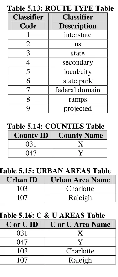
The ROUTE TYPE table, Table 5.13, associates a code with each type of roadway

classifier.

ROUTE TYPE (Classifier Code, Classifier Description)

Classifier Code – numerical value given that relates to a specific type of route Classifier Description – the type of route (interstate, us, state, etc.)

The COUNTIES table, table 5.14, establishes a linkage between the county name and a

standard numerical NC County ID.

COUNTIES (County ID, County name)

County ID – identification number given to a specific county County name – name of the county of interest

The URBAN AREAS table, Table 5.15, gives the urban area name, or city name, for a

numerically designated NC urban area ID.

URBAN AREAS (Urban ID, Urban Area Name)

Urban ID – identification number for a specific urban area, or city Urban Area Name – name of the city or urban area

The C & U AREAS table, Table 5.16 gives the name for a county or urban area when

given a specific county or urban ID.

C & U AREAS (C or U ID, C or U Area Name)

C or U ID – identification number for a specific county or urban area C or U Area Name – name of a specific county or urban area

Table 5.13: ROUTE TYPE Table Classifier

Code

Classifier Description

1 interstate

2 us

3 state

4 secondary 5 local/city 6 state park 7 federal domain

8 ramps

9 projected

Table 5.14: COUNTIES Table

County ID County Name

031 X

047 Y

Table 5.15: URBAN AREAS Table

Urban ID Urban Area Name

103 Charlotte 107 Raleigh

Table 5.16: C & U AREAS Table

C or U ID C or U Area Name

031 X

047 Y

103 Charlotte 107 Raleigh

5.3 Study Goal

Section 5.1 has provided the structure of Pavement Management’s existing link node system. The goal of this study is to devise ways to move from the existing system described in Section 5.1 to the linear referencing system described in Section 5.2 (as shown in Figure 5.1). This move from the link node system to the LRS system can be accomplished by utilizing the existing link node tables in the Pavement Management Unit database.

The work described herein makes use of the link node database tables to create the LRS routes by generating LRS IDs for all links in the roadway network. This study does not create new database tables with the new LRS. Figure 5.1 shows how the LRS algorithms move from the link node system to the LRS.

Figure 5.1: Route Generation System Architecture

It should be emphasized that it was not a goal of this study to determine whether there is a need for the new LRS system. In a study prior to this it was already concluded that a base LRS system was needed. This work builds on that recommendation by providing insight into how to do it. What this study does is provide the DOT with several LRS configurations to choose from. In addition to multiple configurations, this report also provides an interpretation of the analysis results of the various configurations so that the process of choosing an approach is well founded.

5.4 Study Generalizability

Other states could use this base LRS definition. But, how would they do it? In North Carolina the Pavement Management Unit had a link node database that was available and could be used to generate the LRS routes. Given the results of the study, the selected algorithm can be run using the link node database as input and generating the LRS routes and IDs as output.

Other states might choose a manual approach. In North Carolina the total road mileage is approximately 78,000 miles and the number of roads in the link node database is approximately 195,000. With these large numbers a manual approach is not feasible. However, for a state with fewer roads, a manual approach may indeed be a reasonable approach.

Other ways might exist to create the base LRS. The NC DOT study started with a link node referencing system. Other location referencing systems could be used as the starting point as well. If another state had a different referencing system implemented, that system could be used to generate the LRS.

Link Node Chains

LRS Routes LRS