| INVESTIGATION
The Spread of an Inversion with Migration
and Selection
Brian Charlesworth*,1and Nicholas H. Barton†
*Institute of Evolutionary Biology, School of Biological Sciences, University of Edinburgh, EH9 3FL, United Kingdom and†Institute of Science and Technology Austria, 3400 Klosterneuburg, Austria ORCID IDs: 0000-0002-2706-355X (B.C.); 0000-0002-8548-5240 (N.H.B.)
ABSTRACTWe re-examine the model of Kirkpatrick and Barton for the spread of an inversion into a local population. This model assumes that local selection maintains alleles at two or more loci, despite immigration of alternative alleles at these loci from another population. We show that an inversion is favored because it prevents the breakdown of linkage disequilibrium generated by migration; the selective advantage of an inversion is dependent on the amount of recombination between the loci involved, as in other cases where inversions are selected for as a result of their effects on recombination. We derive expressions for the rate of spread of an inversion; when the loci covered by the inversion are tightly linked, these conditions deviate substantially from those proposed previously, and imply that an inversion can then have only a small advantage.
KEYWORDSinversion; linkage disequilibrium; migration; recombination; selection
K
IRKPATRICK and Barton (2006) proposed an influential model for the spread of an inversion that suppresses re-combination between two or more loci that are under selection in a local population, in the face of the introduction of disfavored alleles by geneflow. Up to now, direct evidence for this model has been lacking, but a recent paper on the highly self-fertilizing plantBoechnera strictaclaims to provide an example (Leeet al. 2017). In this case, an inversion has become common in a hybrid zone between two ecologically distinct subspecies, over an esti-mated time of between 1000 to 4000 generations. But it is hard to see how recombination suppression could confer a significant selective advantage when there is a high level of inbreeding within a population, where the effective recombination rate be-tween a pair of loci is greatly reduced (Nordborg 1997), because the advantage of recombination suppression must depend on the rate of recombination in the initial population.Equation 3 of Kirkpatrick and Barton (2006) was intended to describe the selective advantage to a rare inversion, in terms of the rate of recombinationrbetween adjacent loci, the selective disadvantagessuffered by an immigrant allele, and the rate of
migrationm. For the case of two loci, this equation states that the selective advantage of an inversion,sl, is approximately equal to
2rm/(2r+ms). Ifms,,r,slm, and is only weakly dependent
onr. Atfirst sight, this suggests that theB. strictaexample could indeed be explained by their model, although Kirkpatrick and Barton did point out that the selective advantage of an inversion should tend to zero as the recombination rate becomes small.
This note re-examines the Kirkpatrick-Barton model. Two main conclusions are reached. First, the condition for the spread of an inversion is similar to that derived by Charlesworth and Charlesworth (1973) for the case of a randomly mating popula-tion at equilibrium under epistatic selecpopula-tion—linkage disequilib-rium (LD) must be present among the loci subject to selection. Second, Equation 3 of Kirkpatrick and Barton is wrong, presum-ably because of an error in its derivation (the existence of an error in this equation was previously pointed out by Bürger and Akerman (2011)). The denominator is (2r+ms), which is dimensionally inconsistent in the continuous time version of the model, in which the coefficientsr,mandsall have dimensiont21. Using the correct
expression, the selective advantage of an inversion becomes very small when the effective recombination rate is small. This casts some doubt on the interpretation of their data by Leeet al.(2017). Following Kirkpatrick and Barton (2006), we use a model of a haploid species with a focal deme subject to migration from a source deme, with migration rateminto the focal deme. Alleles at two or more loci are assumed to be atfixation in the source Copyright © 2018 by the Genetics Society of America
doi:https://doi.org/10.1534/genetics.117.300426
Manuscript received October 23, 2017; accepted for publication November 14, 2017; published Early Online November 20, 2017.
1Corresponding author: Institute of Evolutionary Biology, School of Biological
deme, and are disfavored by selection in the focal deme. While this model does not fully describe what happens with diploidy, it should provide a good approximation to the dynamics of a highly inbred population, where selection is predominantly among homozygous genotypes. We assume that migration is sufficiently weak in relation to selection that the disfavored alleles in the focal population are kept rare, which greatly sim-plifies the calculations. With this low migration assumption, the model is equivalent to the case of two demes with selection in opposite directions (Moran 1962, pp. 173–175; Charlesworth and Charlesworth 2010, p. 146). Wefirst consider the case of a pair of selected loci, allowing for the possibility of epistasis in
fitness, and then analyze the multi-locus case with additive
fitness effects. A treatment that relaxes the assumption of low migration is given in the Appendix, which is equivalent to the analysis of the diploid model with no dominance or epistasis by Bürger and Akerman (2011). Our mainfindings for the two-locus case when epistasis is absent are equivalent to those of Bürger and Akerman with weak migration.
Results for Two Selected Loci with Low Migration
The state of the initial population
Here, we assume two loci, 1 and 2, with alleles Aiand aiat locusi.
The relativefitnesses of the four haplotypes A1A2, A1a2, a1A2
and a1a2in the focal deme are 1, 12s2, 12s1, and 12s12s2+e,
respectively, wheresiis the selection coefficient against the
dis-favored allele at locusi, andeis a measure of epistasis. Let the frequencies of the four haplotypes in the focal demeibex1,x2,
x3, andx4; the frequencies of alleles Aiand aiat locusiarepiand
qi, respectively. The coefficient of LD isD=x1x42x2x3.
Selec-tion is assumed to be sufficiently strong compared with migra-tion that second-order terms in the frequencies of the disfavored haplotypes can be neglected, but sufficiently weak that second-order terms in the selection parameters are negligible. We writeli = m/sias a measure of the relative strength of
migra-tion and selecmigra-tion at locusi; given our assumptions,li ,, 1.
Even with an additivefitness model, the changes in allele fre-quencies at one locus are not independent of the frefre-quencies of the alleles at the other locus when there is LD generated by migra-tion. The magnitude of this LD at equilibrium is given in Equa-tion 1 below (a simple derivaEqua-tion is provided in the Appendix):
D* m
rþs1þs22e (1)
Note that asterisks are used to denote the equilibrium values of variables.
Substituting from Equation 1 into Equations A2, we get:
q*
1l1½12ðs22eÞ
rþs1þs22eÞ (2a)
q*
2l2½12ðs12eÞ
rþs1þs22eÞ (2b)
With close linkage, such thatr,,s1+s22e, the equilibrium
frequencies of the disfavored alleles are substantially lower than
the values with D* = 0. Whens1 =s2 =s and e = 0, the
symmetrical additivefitness case considered by Kirkpatrick and Barton (2006), these frequencies approachm/(2s) asrtends to zero. The equilibrium meanfitness of the population is greater than the value with no LD, 122m; it approaches 12masr tends to zero. In general, the equilibrium meanfitness is given by:
w*¼12s1q*
12s2q*2þeðq*1q*2þD*Þ
122mþmðs1þs22eÞ=ðrþs1þs22eÞ (3)
Conditions for the spread of an inversion
We now consider the introduction into haplotype 1 of an inversion that completely suppresses crossing over between the two loci. Let the frequency of the inverted haplotype in the focal deme bexI. Then, assuming that the system is
ini-tially at equilibrium, and, using Equations 3 and A3a to de-termine its change in frequency, we obtain:
DxIxI½ð12w*Þ2m xImr=ðrþs1þs22eÞ
¼xIrD* (4)
This is equivalent to Equation 5.2 of Bürger and Akerman (2011) for the corresponding continuous time model without epistasis. The multiplicand of xIprovides a measure of the
selective advantage of the inversion,sI, which corresponds to
the quantityl 2 1 in Kirkpatrick and Barton (2006). This expression shows thatsIis equal to the difference
be-tween the migration load at equilibrium, ð12w*Þ;and the migration load experienced by the inversion, m. This differ-ence depends on the existdiffer-ence of LD in the initial population, as can be seen from the last term in Equation 4. However, with loose linkage, LD is inversely proportional to the recombina-tion rate, and the rate of increase given by Equarecombina-tion 4 is nearly independent ofr, and equal tom, the value for loose linkage given by Equation 1 of Kirkpatrick and Barton (2006). Positive epistasis (e . 0) increases the selective advantage of an in-version, whereas negative epistasis (e , 0) has the opposite effect. As in other situations where reduced recombination is favored by selection, a rare modifier of recombination cannot have a selective advantage in the absence of LD in the initial population, since recombination has no effect on changes in haplotype frequencies in the absence of LD (Feldman 1972; Charlesworth and Charlesworth 1973).
The selective advantage to the inversion given by the right-hand side of Equation 4 differs substantially from that given by the expression forlin Equation 3 of Kirkpatrick and Barton (2006) for the case whens1 = s2 = sande = 0. That
givessl = 0.00024 compared with 0.0091 from the formula of
Kirkpatrick and Barton. The Appendix gives the exact two-locus solution in the continuous-time limit, for the case of additive selection; essentially the same results were derived previously by Bürger and Akerman (2011) for the diploid model without dominance.
The multi-locus case with additivefitnesses:For simplicity, only the case when each locus has the same selection co-efficient,s, will be considered, as in Kirkpatrick and Barton (2006). The same notation as above is used, except that there are now nloci under selection; the recombination rate be-tween lociiandjisrij, and the coefficient of LD between these
loci in the focal deme isDij. Equations 3 of Barton (1983) can
be used to be obtain an exact solution, assuming weak selec-tion. Here, we provide a heuristic treatment of the problem, assuming additivefitness effects.
With tight linkage, and assuming that migration is much weaker than selection, the focal population will be composed predominantly of haplotype 1, carrying the favored allele Ai
at each of thenloci in the chromosomal region under con-sideration; the immigrant haplotypes all have allele ai at
these loci. With these assumptions, haplotype 1 will be bro-ken down by recombination at rate Rx1x0, where R is the
probability of at least one recombination event in the region in question,x1is the frequency of haplotype 1, andx0is the
frequency of the complementary, immigrant haplotype. For the initial population, we thus have:
Dx1x1ð12w2m2Rx0Þ (5)
At equilibrium, the selective advantage of an inversion in haplotype 1 is thus given by:
sI¼12w*2mRx*0 (6a)
But, with tight linkage, the system behaves very like a single locus with net selection coefficientS = ns, so that:
x* 0
m SþOðRÞ
Substituting this into Equation 6a, we obtain:
sI
mR
S (6b)
If the loci are equally spaced along the chromosome, with distancerbetween each pair,R = (n21)r(assuming that terms inr2can be neglected) and:
sImðn21Þr
ns (6c)
Withn ..2,sIis largely determined by the frequency of
recombination between adjacent loci, and the strength of selection at each locus.
For the opposite extreme of free recombination, the pro-cedure of neglecting LD used by Kirkpatrick and Barton
(2006) can be followed. Because each locus then causes an equilibrium reduction infitness ofm, the equilibrium mean
fitness of the focal population is1 2 nm; substituting this into Equation 6a gives their multi-locus expression forsIwith
loose linkage,sI ðn21Þm:
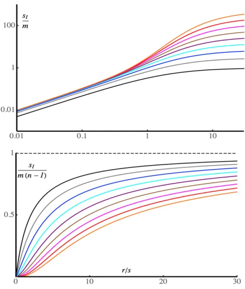
Figure 1 shows how the advantage of the inversion de-pends on the rate of recombination relative to selection, r = r/s. An exact treatment using Equations 3 of Barton (1983) was applied in order to generate the curves. When r , 0.5, we have sI , m and sI approaches at most
mr/(s 2 r) as the number of loci increases. In this regime, all the loci are in strong LD, the migration load is close tom, and the inversion does not have much of an advantage. When r . 1, the migration load, and, hence, the advantage to the inversion, can be much larger (right-hand side of the upper panel in Figure 1), especially when many loci are involved. The advantage is now a substantial fraction ofsI = m(n21),
the limiting value with loose linkage (lower panel of Figure 1).
Discussion
Here, we will briefly consider the implications of these results for the interpretation of the results of Leeet al.(2017) on the Figure 1 The selective advantage of an inversion,sI, in the limit of low
migration, forn = 2, 4, 8,. . ., 256, 512 loci, plotted againstr/s. The upper plot shows sI/m on a log-log scale, with the number of loci
increasing from bottom to top. The lower plot showssI/m(n21), with
inversion polymorphism ofB. stricta. Equations 4, 6c, and A8 imply that, when there is a high rate of self-fertilization in the population, this mechanism can provide only a weak selective advantage for an inversion. This follows from the fact that, with an inbreeding coefficient offresulting from a departure from random mating within a population, the effective re-combination rate that replaces r is (1 2 f)r (Nordborg 1997; Charlesworth and Charlesworth 2010, p. 382). Song et al.(2006) obtained an estimate off = 0.90 forB. stricta, using data on microsatellite genotypes. The effective recom-bination rate for this example is thus about one-tenth of the rate of recombination per meiosis, and the advantage of the inversion would be0.1mr/sif a moderate number of loci were covered by it.
Because extensive differentiation between the two subspecies at loci under selection requiresm , , s, the selective advan-tage to an inversion is likely to be substantially,0.001 if the selected loci are,10 cM apart. This implies a chance of only
0.002 that a single new inversion would become estab-lished in the population as a result of selection (Haldane 1927), so that many independent mutational events gener-ating an inversion in the chromosomal region in question would be needed before one succeeded in spreading to a high frequency. While Lee et al.(2017) provide convincing evi-dence that the inversion is associated with locally adaptive alleles, their interpretation in terms of the Kirkpatrick and Barton (2006) model thus has little or no advantage over a scenario in which an inversion that spread to an intermediate frequency by drift happened to pick up a selectively favorable mutation, and was then driven to a high frequency by hitchhiking.
Acknowledgments
We thank the Edinburgh Evolutionary Genetics Laboratory Group, especially Ben Jackson, for useful comments, and an anony-mous reviewer, Reinhard Bürger, Mark Kirkpatrick, and Thomas Mitchell-Olds for their comments on the draft manuscript.
Literature Cited
Barton, N. H., 1983 Multilocus clines. Evolution 37: 454–471. Bürger, R., and A. Akerman, 2011 The effects of linkage and gene
flow on local selection in a continent-island model. Theor. Popul. Biol. 80: 272–288.
Charlesworth, B., and D. Charlesworth, 1973 Selection of new in-versions in multi-locus genetic systems. Genet. Res. 21: 167–183. Charlesworth, B., and D. Charlesworth, 2010 Elements of Evolu-tionary Genetics. Roberts and Company, Greenwood Village, CO. Feldman, M. W., 1972 Selection for linkage modification: 1.
Ran-dom mating populations. Theor. Popul. Biol. 3: 324–346. Haldane, J. B. S., 1927 A mathematical theory of natural and
artificial selection. Part V. Selection and mutation. Proc. Camb. Philos. Soc. 23: 838–844.
Kirkpatrick, M., and N. Barton, 2006 Chromosome inversions, lo-cal adaptation and speciation. Genetics 173: 419–434. Lee, C.-R., B. Wang, J. P. Mojica, T. Mandakova, K. V. S. K. Prasad
et al., 2017 Young inversion with multiple linked QTLs under selection in a hybrid zone. Nat. Ecol. Evol. 1: 119.
Moran, P. A. P., 1962 The Statistical Processes of Evolutionary The-ory. Oxford University Press, Oxford.
Nordborg, M., 1997 Structured coalescent processes on different time scales. Genetics 146: 1501–1514.
Song, B.-H., M. J. Clauss, A. Pepper, and T. Mitchell-Olds, 2006 Geographic patterns of microsatellite variation inBoechnera stricta, a close relative ofArabidopsis. Mol. Ecol. 15: 357–369.
Appendix
Two-Locus Results: Approximation for Weak Migration Relative to Selection
The difference in the frequency of allele A2at locus 2 between carriers of alleles A1and a1is equal toD/p1q1(Charlesworth and
Charlesworth 2010, p. 410), so that the effect onfitness of substituting A1for a1at locus 1 through its associated effect on
locus 2 is equal to (s2 2 e)D/p1q1; this term can be added to the directfitness effect of the substitutions1. Ifq1 ,, 1, the net
selective advantage of A1over a1is given by:
dw1 ½s1þ ðs22eÞD=q1 (A1a)
Similarly, the selective advantage of A2over a2is:
dw2 ½s2þ ðs12eÞD=q2 (A1b)
The change inqidue to selection is approximately equal toqidwi; the change due to migration is approximately equal tom
whenm ,, si, as is assumed here. At equilibrium (denoted by asterisks), the equilibrium frequencies of the disfavored alleles
are given by:
q*
1l12½ðs22eÞD*
s1 (A2a)
q*2l22½ðs12eÞD*s2 (A2b)
The recursion relations for each haplotype can be used to determineD*. If the source deme isfixed for haplotype 4, the haplotype recursion relations with weak selection are as follows:
Dx1x1ð12wÞ2rD2mx1 (A3a)
Dx2x2ð12s22wÞ þrD2mx2 (A3b)
Dx3x3ð12s12wÞ þrD2mx3 (A3c)
Dx4x4ð12s12s2þe2wÞ2rDþmð12x4Þ (A3d)
wherewis the population meanfitness. We have:
DDx4Dx1þx1Dx42x3Dx22x2Dx3 (A4)
Writing the haplotype frequencies asx1=p1p2+D,x2=p1q22D,x3=q1p22D,x4=q1q2+D, using Equations A1, and
assuming that the population is close to equilibrium, the selection terms in Equation A4 give:
DDsDð222w2s12s2Þ þex4 2Dðs1þs22eÞ (A5a)
Provided that thefitness of A1A2is greater than that of a1a2(so that selection is purely directional), the multiplicand ofDis
negative.
The recombination term isDDr = 2rD. This leaves the migration term to be evaluated, which is given by:
The net change inDnear equilibrium is thus approximately:
DD 2Dðrþs1þs22eÞ þm (A6)
Equating this to zero gives Equation 1 of the main text.
Two-Locus Results: Exact Solution with Additive Selection
Here, we present the exact solution for the case when all processes are slow, withm,rD,s ,, 1, treating the population as evolving in continuous time, as in Bürger and Akerman (2011), whose treatment of the diploid model with semi-dominance is equivalent to this: their Eqs. 2.5 are equivalent to our A7 below. This analysis shows how the advantage of an inversion changes as migration increases, toward a critical value at which it overwhelms selection. In this case, the rates of change of allele frequencies and LD, and the selective advantage of the inversion, are given by:
_
p1¼2mp1þs1p1q1þs2D _
p2¼2mp2þs2p2q2þs1D _
D¼2½rþmþs1ðp12q1Þ þs1ðp22q2ÞDþmp1p2
sl¼s1q1þs2q22m¼m2D
s2
p1þ s1 p2
(A7)
Provided that migration is not too high, both locally favored alleles can be maintained in the focal deme, giving the following equilibrium results:
q*
1¼ ½ðrþs1Þ 22
s22þ4mr2ðrþs12s2ÞA8rs1
q*
2¼ ½ðrþs2Þ 22
s2
1þ4mr2ðrþs22s1ÞA
8rs2
D*¼ mp
* 1p*2
rþmþs1ð122q1*Þ þs1ð122q*2Þ
sl¼ ðrþs1þs22AÞ=4
A¼
ffiffiffiffiffiffiffiffiffiffiffiffiffiffiffiffiffiffiffiffiffiffiffiffiffiffiffiffiffiffiffiffiffiffiffiffiffiffiffiffiffiffi ðrþs1þs2Þ228mr
q
(A8)
The critical migration rate, above which one or both alleles are swamped, is:
mc¼ ðrþs1þs2Þ2
8r (A9)
The maximum advantage to the inversion is when migration is just below this critical value:
slm¼
1
4ðrþs1þs2Þ ¼
ffiffiffiffiffiffiffiffiffiffiffiffiffi
rmc=2
p
(A10)
With loose linkage, such thatm,s,,r, the advantage to the inversion can be written as:
sl
mr