Kernel Machine Regression in Presence of Multivariate Response with Application to Genetic Data.

(1)

ABSTRACT

ZHAO, JING. Kernel Machine Regression in Presence of Multivariate Response with Application to Genetic Data. (Under the direction of Arnab Maity and Jung-Ying Tzeng.)

Genomic association studies involve studying the relationship between genetic covariates and phenotypes. When in presence of multiple phenotypes, it is believed that joint analysis of these phenotypes is more beneficial in detecting genes that might have genetic effects, comparing with univariate analysis. Kernel Machine Regression (KMR) recently has gained its popularity in association studies as a useful dimension reduction tool and an efficient modelling scheme. It models the genetic covariates nonparametrically and aim to capture complicated interactions among the covariates in addition to main effects. However, most of the available literature consider the case when the response variable is univariate. In this dissertation, we develop estimation and testing procedures for kernel machine regression when we have multivariate response variables and analyse various genetic data applications.

Chapter 2 focuses on studying the joint effect of a set of single nucleotide polymorphisms (SNPs) on multivariate phenotypes. In this chapter, we apply the kernel machine framework to model the genetic markers together to capture the underlying genetic structure more precisely, and we use multivariate regression to preserve the possible correlation between the phenotypes. Specifically, we construct a semiparametric regression model with multiple responses, where the demographic and clinic covariates are modelled parametrically and the joint effects of genetic covariates are modelled nonparametrically using kernel machines. We develop estimation and testing procedures in this framework and conduct simulation studies to evaluate the performance of our proposed methodology. To demonstrate the benefits of applying multivariate analysis, we compare our method with Univariate Kernel Machine (UVKM) procedure to evaluate both estimation and testing. The utility of the proposed method is demonstrated using data from a lymphoblastoid cell lines (LCLs) study.

(2)

inves-tigating global association between DNA copy number profiles from multiple myeloma (MM) patients and two relevant biomarkers.

(3)

(4)

Kernel Machine Regression in Presence of Multivariate Response with Application to Genetic Data

by Jing Zhao

A dissertation submitted to the Graduate Faculty of North Carolina State University

in partial fulfillment of the requirements for the Degree of

Doctor of Philosophy

Bioinformatics

Raleigh, North Carolina

2014

APPROVED BY:

Matthew Breen Alison Motsinger

Arnab Maity

Co-chair of Advisory Committee

Jung-Ying Tzeng

(5)

DEDICATION

(6)

BIOGRAPHY

(7)

ACKNOWLEDGEMENTS

First of all, I would like to thank my advisor Arnab Maity for his supervision and professional guidance on my research and dissertation work. None of these would be possible without his patience, time, encouragement and inspiration. I’d like to thank my committee members, Jung-Ying Tzeng, Matthew Breen, Alison Motsinger and Alex Graves. I want to thank Matthew for his great suggestions on CNAs project, and I’d like to express my sincere gratitude to Alison for providing LCLs data and giving me detailed comments on my dissertation.

I’d like to thank my department for the constant financial support to my PhD study and thank Spencer Muse and all the faculty and staff at Bioinformatics Research Center for their patience and kindness in answering my tedious questions and in helping me dealing with school issues.

(8)

TABLE OF CONTENTS

LIST OF TABLES . . . vii

LIST OF FIGURES . . . x

Chapter 1 Introduction . . . 1

1.1 Genome-Wide Association Study (GWAS) . . . 1

1.2 Multi-marker Association Analysis . . . 3

1.3 Multivariate Phenotype Association Analysis . . . 4

1.4 Data Motivations . . . 6

1.5 Summary . . . 7

Chapter 2 Multivariate Kernel Machine Regression with Vector-Valued Co-variates . . . 9

2.1 Introduction . . . 9

2.2 Multivariate Kernel Machine Regression . . . 11

2.2.1 Estimation of model components . . . 12

2.2.2 Standard Error Estimation and Penalty Parameter Selection . . . 13

2.2.3 Prediction . . . 15

2.3 Hypothesis Testing . . . 15

2.4 Simulation Study . . . 16

2.4.1 Estimation . . . 18

2.4.2 Testing . . . 23

2.5 Data Analysis . . . 26

2.6 Discussion . . . 33

Chapter 3 Testing for Effects of Functional Covariates on Multivariate Re-sponses . . . 35

3.2 Methodology . . . 38

3.2.1 Testing in Multi-response Functional Linear Model . . . 39

3.2.2 Testing in Multi-response Functional Nonlinear model . . . 40

3.2.3 Testing in presence of multiple candidate kernels with multivariate responses 42 3.3 Simulation Study . . . 43

3.3.1 Design . . . 43

3.3.2 Results . . . 44

3.4 Data Analysis . . . 48

Chapter 4 Multivariate Kernel Machine SNP Set Tesing Under Multiple Can-didate Kernels . . . 56

4.2 Material and Methods . . . 58

(9)

4.2.2 Testing for the Marker-Set Effect . . . 60

4.2.3 Composite Kernels . . . 60

4.2.4 Perturbation Based Inference . . . 62

4.3 Simulation Study . . . 63

4.4 Results . . . 66

Chapter 5 Conclusions and Future Directions . . . 72

REFERENCES . . . 75

APPENDICES . . . 85

Appendix A Additional Material for Testing for Effects of Functional Covariates on Multivariate Responses . . . 86

A.1 Simulation Results . . . 86

A.2 Penetrance Plots . . . 91

(10)

LIST OF TABLES

Table 2.1 Frequency of genotypes used in the simulation study. . . 17 Table 2.2 Estimation ofβ’s for simulation study in Section 2.4. We report the empirical

bias (Bias), empirical standard deviation (sd), estimated standard errors aver-aged over 1000 simulations (se) and coverage probabilities (Coverage) of 95% confidence intervals. The biases are calculated from comparing the estimated values with the true values of β’s, (0.7,1),(0.7,1),(0.7,1). The original values are multiplied by 100 and rounded to their 2nd decimal places. . . 20 Table 2.3 Model Evaluation for measure the accuracy of the estimate of h. Displayed

are the two M’s defined in Section 2.4, the correlation between the estimated Y and its true value, and the slope and intercept of fitting the simple linear modelhb =h. . . 21

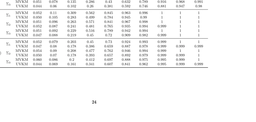
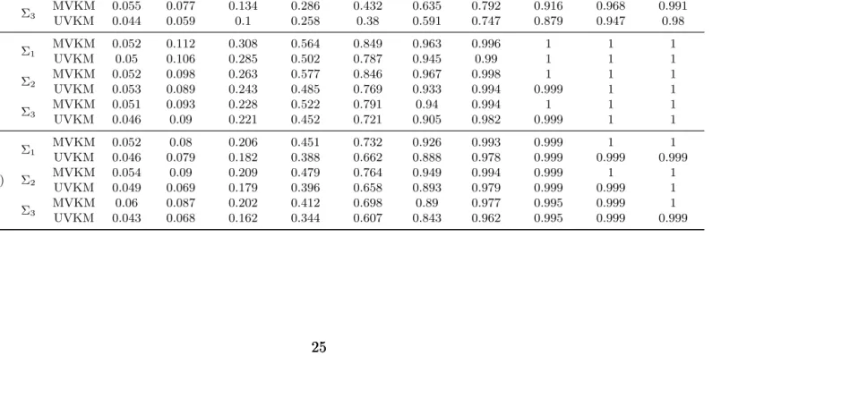
Table 2.4 Simulation results for testing for one h function. Displayed are the power of our test (MVKM) along with multiple univariate testing with Bonferroni correction (UVKM) for different settings (α= 0.05). . . 24 Table 2.5 Simulation results for testing for two h functions. Displayed are the power

of our test (MVKM) along with multiple univariate testing with Bonferroni correction (UVKM) and Type I errors (δ = 0) for different scenarios (α= 0.05). 25 Table 2.6 Summary of the top 10 windows with the most significant results on

Chromo-some 10 . . . 29

Table 4.1 Haplotype frequencies for the Renin gene. . . 64 Table 4.2 Simulation settings forh= (hi1, hi2, hi3)T. . . 65

Table B.1 Simulation results forp= 3 andh=h1 (main effect). Displayed are the power

of MVKM test using linear (Lin), quadratic (Quad), IBS (IBS) kernel, com-posite kernel based on Wu et al. (2013)’s proposed weights (Wu), comcom-posite kernel based on P0 (Comp1), composite kernel based on maximum of

abso-lute entries for each kernel (Comp2) and perturbation-based method (Ptb), as described in simulation section, forα= 0.05. . . 95 Table B.2 Simulation results for p = 3 and h = h2 (interaction). Displayed are the

power of MVKM test using the linear (Lin), quadratic (Quad), IBS (IBS) kernel, composite kernel based on Wu et al. (2013)’s proposed weights (Wu), composite kernel based onP0 (Comp1), composite kernel based on maximum

(11)

Table B.3 Simulation results forp= 3 andh=h3 (main and interaction). Displayed are

the power of MVKM test using the linear (Lin), quadratic (Quad), IBS (IBS) kernel, composite kernel based on Wu et al. (2013)’s proposed weights (Wu), composite kernel based onP0 (Comp1), composite kernel based on maximum

of absolute entries for each kernel (Comp2) and perturbation-based method (Ptb), as described in simulation section, for α= 0.05. . . 97 Table B.4 Simulation results forp= 3 andh=h4 (mix effect). Displayed are the power

of MVKM test using the linear (Lin), quadratic (Quad), IBS (IBS) kernel, , mixed kernel (Mix), composite kernel based on Wu et al. (2013)’s proposed weights (Wu), composite kernel based onP0 (Comp1), composite kernel based

on maximum of absolute entries for each kernel (Comp2) and perturbation-based method (Ptb), as described in simulation section, for α= 0.05. . . 98 Table B.5 Simulation results for p = 3 and h =h5 (complex effect). Displayed are the

of absolute entries for each kernel (Comp2) and perturbation-based method (Ptb), as described in simulation section, for α= 0.05. . . 99 Table B.6 Simulation results for p = 5 and h = h1 (main effect). Displayed are the

of absolute entries for each kernel (Comp2) and perturbation-based method (Ptb), as described in simulation section, for α= 0.05. . . 100 Table B.7 Simulation results for p = 5 and h = h2 (interaction). Displayed are the

of absolute entries for each kernel (Comp2) and perturbation-based method (Ptb), as described in simulation section, for α= 0.05. . . 101 Table B.8 Simulation results forp= 5 andh=h3 (main and interaction). Displayed are

the power of MVKM test using the linear (Lin), quadratic (Quad), IBS (IBS) kernel, composite kernel based on Wu et al. (2013)’s proposed weights (Wu), composite kernel based onP0 (Comp1), composite kernel based on maximum

of absolute entries for each kernel (Comp2) and perturbation-based method (Ptb), as described in simulation section, for α= 0.05. . . 102 Table B.9 Simulation results forp= 5 andh=h4 (mix effect). Displayed are the power

of MVKM test using the linear (Lin), quadratic (Quad), IBS (IBS) kernel, mixed kernel (Mix), composite kernel based on Wu et al. (2013)’s proposed weights (Wu), composite kernel based onP0 (Comp1), composite kernel based

(12)

Table B.10 Simulation results for p = 5 and h =h5 (complex effect). Displayed are the

(13)

LIST OF FIGURES

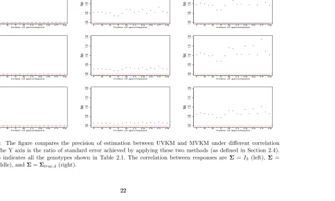
Figure 2.1 The figure compares the precision of estimation between UVKM and MVKM under different correlation settings. The Y axis is the ratio of standard error achieved by applying these two methods (as defined in Section 2.4). The x axis indicates all the genotypes shown in Table 2.1. The correlation between responses are Σ=I3 (left),Σ=Σtrue,3(middle), and Σ=Σtrue,4 (right). . . 22

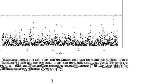
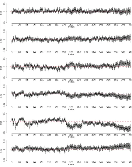
Figure 2.2 Testing results of chromosome 10 on temozolomide. Sliding window scheme is applied and association study is conducted to test for the SNP-set ef-fect within each window on temozolomide at six different concentrations.

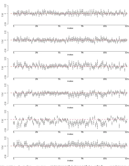
−log₁₀(p-value) is plotted for each corresponding window. The red dashed line indicates the significant level for Bonferroni correction (2.2×10−5) and the red solid line is the significance level for GWAS (5×10−8). . . 30 Figure 2.3 Estimation of window 2192 (131.32Mb - 131.42Mb) of LCLs study. The

fig-ures display the individual point estimates of h1, . . . , h6 along with their 95% confidence intervals. . . 31 Figure 2.4 Estimation of window 2194 (131.42Mb - 131.51Mb) of LCLs study. The

fig-ures display the individual point estimates of h1, . . . , h6 along with their 95% confidence intervals. . . 32

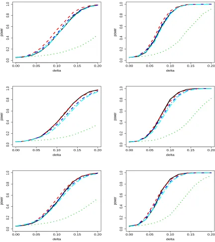
Figure 3.1 Results of simulation for case 1 and p = 2 as described in Section 3.3.1. Displayed are the power curve for LRT (solid black), MVKM test using the linear kernel (red dashed), the quadratic kernel (green dotted), composite kernel method (blue dot-dashed) and perturbation-based method (cyan long-dashed). The left three plots are n = 100 and the right are n = 200. The top two plots are for the cases when responses are independent (Σtrue,1), the

middle ones are for low correlation (Σtrue,2) and the bottom two are for high

correlation (Σtrue,3). . . 46

Figure 3.2 Results of simulation for case 2 and p = 2 as described in Section 3.3.1. Displayed are the power curve for LRT (solid black), our procedure with linear kernel (red dashed), with quadratic kernel (green dotted), average ker-nel method (blue dot-dashed) and perturbation-based method (cyan long-dashed). The left three plots are n = 100 and the right are n = 200. The top two plots are for the cases when responses are independent (Σtrue,1), the

(14)

Figure 4.1 Simulation results for p = 3 and h = h3 (mixed). Displayed are the power

curves of MVKM test using the linear (Lin), quadratic (Quad), IBS (IBS) kernel, composite kernel based on Wu et al. (2013)’s proposed weights (Wu), composite kernel based onP0 (Comp1), composite kernel based on maximum

of absolute entries for each kernel (Comp2) and perturbation-based method (Ptb), as described in simulation section, for α = 0.05. The left three plots are n = 100 and the right are n = 200. The top two plots are for the cases when responses are independent (Σ1), the middle ones are for low correlation

(Σ2) and the bottom two are for high correlation (Σ3). . . 69

Figure 4.2 Simulation results for p= 3 and h =h5 (complex effect). Displayed are the

power curves of MVKM test using the linear (Lin), quadratic (Quad), IBS (IBS) kernel, composite kernel based on Wu et al. (2013)’s proposed weights (Wu), composite kernel based on P0 (Comp1), composite kernel based on

maximum of absolute entries for each kernel (Comp2) and perturbation-based method (Ptb), as described in simulation section, forα= 0.05. The left three plots are n = 100 and the right are n = 200. The top two plots are for the cases when responses are independent (Σ1), the middle ones are for low

correlation (Σ2) and the bottom two are for high correlation (Σ3). . . 70

Figure A.1 Power for Functional Linear Model. The left column is when n = 100 and

n= 200 is on the right. The first row is when the responses are independent, the second row is when there are low correlations between the responses and the third is when they are highly correlated. We applied Wilk’s, Roy, Pillai, Hotelling-Lawley test, as well as univariate test with Bonferroni correction. The plots show that LRT test, Wilk’s, Pillai and Hotelling-Lawley tend to have similar performances. The Roy test has more power but also larger Type I error. The univariate test with Bonferroni correction has similar per-formance as LRT test for independent cases, however, it loses power when the multivariate responses are dependent. . . 87 Figure A.2 Power for case 1,p = 2 andn= 200 (described in Section 3.3.1). Displayed

are the power curve for MVKM test using the linear kernel (red dashed), linear model with the mean of the covariates in the model (black dot-dashed) and linear model with covariates as vector-valued explanatory variables in the model (solid blue). The three plots corresponds to the cases when the responses are independent (Σtrue,1, top left) in low correlation (Σtrue,2, top

(15)

Figure A.3 Results of simulation for case 1 and p = 5 as described in Section 3.3.1. Displayed are the power curve for LRT (solid black), MVKM using the lin-ear kernel (red dashed), the quadratic kernel (green dotted), composite ker-nel method (blue dot-dashed) and perturbation-based method (cyan long-dashed). The left three plots are n = 100 and the right are n = 200. The top two plots are for the cases when responses are independent (Σtrue,1), the

Figure A.4 Results of simulation for case 2 and p = 5 as described in Section 3.3.1. Displayed are the power curve for LRT (solid black), MVKM test using the linear kernel (red dashed), the quadratic kernel (green dotted), composite kernel method (blue dot-dashed) and perturbation-based method (cyan long-dashed). The left three plots are n = 100 and the right are n = 200. The top two plots are for the cases when responses are independent (Σtrue,1), the

Figure A.5 Penetrance plots showing the frequency of gain and loss of genomic regions from MM patients. X-axis represents each chromosome, and the y-axis indi-cates the % gain or loss of the corresponding genomic region. Gains are shown in blue and losses in red. . . 92 Figure A.6 Penetrance plots showing the frequency of gain and loss of selected significant

(16)

Chapter 1

Introduction

In this introduction chapter, I give a brief overview of Genome-Wide Association Study (GWAS). I describe the situation when multivariate phenotypes and multiple genetic markers are involved in association study and the reason why they attract current research interests. I introduce the data sets in Chapter 2 and Chapter 3, which fits the situation, and I explain how the data sets serve as motivations to my work in this dissertation.

1.1 Genome-Wide Association Study (GWAS)

During the past decades, genetic architectures and genetic variations of a variety of complex traits and phenotypes have been studied, such as gene expression, susceptibilities to common disease and response to therapeutic treatment. One of the most powerful tools for investigating the genetic architecture of the traits is Genome-wide association studies (GWAS), in which hundreds of thousands of single nucleotide polymorphisms (SNPs) are assayed among hundreds or thousands of individuals. GWAS in theory provide an unbiased way to demonstrate the relationship between genome-wide genetic variants and the phenotypic traits of interest. They correlate allele frequencies at each of several hundred thousand markers spaced throughout the genome with trait variation in a population-based sample. GWAS is based on the premise that a causal variant is located in a haplotype, and therefore a marker allele in linkage disequilibrium (LD) with the causal variant should show an association with a trait of interest.

(17)

and assured the feasibility and efficiency of GWAS approach to find unknown disease associated variants.

There were various findings in GWAS in succeeding years. One of them was that KCNQ1 was found to be a strong candidate for conferring susceptibility to type 2 diabetes (T2D) (Yasuda et al. (2008)). In the study, they carried out a multistage GWAS of T2D in Japanese individuals, with a total of 1,612 cases and 1,424 controls and a million SNPs, and found that the most significant association was obtained with SNPs in KCNQ1. The association of KCNQ1 with T2D was then replicated in populations of Korean, Chinese and European ancestry. Moreover, a meta-analysis of three GWAS in 13,685 individuals of European ancestry found five genes to be associated with QT interval, which is a heritable risk factor for sudden cardiac death and drug-induced arrhythmias, and KCNQ1 was one of them (Newton-Cheh et al. (2009)). These findings further revealed the pleiotropic effect of gene or genetic locus influences on multiple traits. In 2007, the Wellcome Trust Case Control Consortium (WTCCC) study examined the genetic basis of seven complex diseases. A total of about 17,000 samples, 2,000 cases for each of the diseases and 3,000 shared controls, were genotyped for half a million SNPs (Burton et al. (2007)). This study was established as the landmark GWAS in 2007 because it identified many novel genes and genetic loci that later were replicated in subsequent studies (Parkes et al. (2007), Todd et al. (2007), Rioux et al. (2007)). More importantly, the WTCCC study also addressed some crucial methodological and analytical issues in designing and conducting a GWAS.

It is true that the associations that have been identified so far still have very limited pre-dictive value, but researchers are still in the infancy of understanding the genetics of complex diseases, and what have been uncovered so far has nonetheless been valuable. A great many novel genetic loci for many complex diseases have been found in enormous studies looking at hundreds of thousands of markers throughout the genome, and systematically, independently replicated in subsequent studies using stringent statistical approaches. GWAS is especially suited to the identification of common variants with modest to large effects on phenotype (McCarthy et al. (2008)). In addition, the findings have provided new insights into the biological pathways of several complex disease, even when GWAS largely depend on LD between markers and disease causative variants.

(18)

1.2 Multi-marker Association Analysis

The advances in current high-throughput biotechnology makes large-scale of genetic data avail-able for association studies. For example, Phase II HapMap genotyped over 3.1 million human SNPs in 270 individuals from four geographically diverse populations, which includes 25% -30% of common SNP variation in the populations (Frazer et al. (2007)). The typical strategy is to individually analyse single genetic marker at one time and then apply standard procedures to control for multiple comparisons (Nyholt (2004), Li and Ji (2005)). However, this procedure is not powerful due to its inability to capture the interactions between the variants.

One class of approaches involving association analysis of multiple markers is haplotype-based methods. Association studies based on linkage disequilibrium (LD) offer promising approaches for detecting genetic variants and methods based on haplotypes are believed to provide more power for genetic association mapping (Tzeng and Bondell (2009), Tzeng and Zhang (2007), Huang et al. (2007a), Tzeng et al. (2006), Schaid et al. (2002)). Such haplotype-based methods typically apply multilinear regression to model the effect of the haplotypes on the trait of interest. Unfortunately, the haplotypes for each individuals in studies cannot be easily acquired, and therefore, the haplotype-based methods either have to take extra procedures to deal with the unphased genetic data or have to account for the phase uncertainty in the analysis.

Alternatively, one can use genotype data directly and these methods can be categorized as genotype-based methods. When testing for the joint effect of multiple markers in case-control studies, multivariate HotellingsT2 statistic was proposed by Fan and Knapp (2003), and they compared the mean genotype scores between the cases and controls using theT2 statistic. This procedure is equivalent to a logistic regression. However, the method has its limits in that it suffers from weak power due to large number of degrees of freedom. Later, Schaid et al. (2005) proposed a global statistics that is the maximum of each single marker statistics and obtained the p-value through a permutation procedure. They showed that their method in general performs better than the Hotellings T2 statistic. In their paper, Schaid et al. (2005) also developed another powerful approach, which is basically a non-parametric test based on U-statistics. Their method first measures a score over all markers for pairs of subjects and then compares the averages of these scores between cases and controls. However, note that for these methods, the powers of the statistics are affected by the direction of the genotype scores at each marker (Wang and Abbott (2008)).

(19)

typical dimension reduction approach and can be applied to the association analysis of multiple genetic variants (Wang and Abbott (2008)). Fourier transformation can also be used to reduce the dimension of genetic variants to a set of orthogonal predictors which contain the majority of information found in the markers (Wang and Elston (2007)). However, it is difficult to interpret the result spaces produced by PCA or Fourier transformation.

Another class of methods attempts to address the issue by using notions of pairwise sim-ilarity (Mukhopadhyay et al. (2010), Schaid (2010), Tzeng et al. (2009), Wessel and Schork (2006)), which often is defined as a matrix of genetic similarities for all pairs of subjects. In these methods, the association of the genetic similarities with phenotypes is evaluated in a re-gression framework, typically by variance component methods that treat the similarity matrix as a general covariance structure. Kernel Machine Regression (KMR) methods fall into this class and they compare pairwise similarity in genotypes between individuals with similarity defined through a kernel function, resulting a kernel matrix. Without any specification on the function that models the joint effect of the markers on the traits, KMR approach is able to nonparametrically model the genetic variants based on the kernel matrix.

KMR recently has gained its popularity in association studies as an efficient dimension re-duction tool (Liu et al. (2007), Kwee et al. (2008), Wu et al. (2011), Maity et al. (2012)). In addition, it models the genetic covariates nonparametrically and aims to capture complicated interactions among the covariates in addition to the main effects. In this dissertation, we fa-cilitate the joint evaluation of multiple genetic markers on multivariate phenotypes based on KMR. We develop a semiparametric regression model which models the non-genetic covari-ates parametrically and genetic covaricovari-ates nonparametrically and name it multivariate kernel machine (MVKM) regression.

1.3 Multivariate Phenotype Association Analysis

In genomic association studies, multiple relevant phenotypes are often collected and joint anal-ysis of these phenotypes is preferred with the aim of capturing possible correlation between the phenotypes which will further produce more informative inferences in investigation of disease pathways or larger strengths of association.

(20)

measurements of IgG class antibodies to the exposure of HSV-1, HSV-2 and CMV together can be the traits of interest (Maity et al. (2012)).

It may also be the multiple measurements of the same value for a certain trait of interest. In Chapter 2, the dataset is from a large lymphoblastoid cell lines (LCLs) study, which aims to perform genetic association mapping for 29 chemotherapy drugs (Medina et al. (2008), Brown et al. (2014)). It is known that most chemotherapeutic agents produce cytotoxic effect in cells. To investigate the genetic association of cytotoxicity of the anticancer drugs in different concen-trations, in this study, each cell line was exposed to six different concentrations of each drug and the responses for all the drugs were then assessed. In Chapter 2, the cytoxicity responses to one of the chemotherapy drugs, temozolomide, at six different concentrations are the phenotypes of interest in the analysis.

Another example will be multiple clinical biomarkers that reflect the same characteristic of a disease. In Chapter 3, the data is collected by Multiple Myeloma Research Consortium and we are interested in the prognosis of multiple myeloma (MM) patients, since the range of survival time for MM patients can vary from less than 6 months to more than 10 years. The International Staging System is based on the combination of two clinical biomarkers, β-2 microglobulin and serum albumin, for their three stage classification. Therefore, we consider the two clinical biomarkers as the traits of interest in our analysis on the prognosis of MM patients.

A traditional scheme of testing with multiple phenotypes would be conducting individual test for each phenotype and then correcting for multiple testing. However, the method suffers penalties from multiple testing and result in a decreased power. An alternative to this standard approach is to apply dimension reduction technique to the phenotypes, such as principle com-ponent (PC) approach. It reduces the dimension of the phenotypes into independently principle components of the phenotypes (PCP) and tests for the associations between the markers and the PCP. However, it is quite possible that the PCP have low heritability, and to solve this issue, an alternative method based on principle component of heritability (PCH) has been pro-posed (Klei et al. (2008)), which reduces the phenotypes into a single trait with a heritability higher than any other linear combination of the phenotypes. Nevertheless, the method has the limitation of reducing the effective sample size due to its required cross-validation procedure.

(21)

on them with the ultimate goal of better understanding the etiology of the disease or better capturing the underlying molecular mechanism of the drug cytotoxicity.

1.4 Data Motivations

This research is motivated by two real data applications. The first data set (described in Chapter 2) is from a large LCLs study, which consists of 520 LCLs that are derived from unrelated Caucasian participants of the CAP clinical trail (Medina et al. (2008), Brown et al. (2014)). The main goal of the data analysis is to study the joint effect of SNP-set on cytotoxic response to temozolomide, which can be achieved by applying our proposed multivariate kernel machine (MVKM) framework.

LCLs model recently emerges as a promising model in cancer study. LCLs are established by in vitro transformation of human lymphocytes by Epstein-Barr Virus (EBV). The virus is a human herpesvirus that can infect human B lymphocytes and then drives the cells into perma-nent proliferation, to mimic the status of cancer cells. As described in Section 1.3, cytotoxicity to anticancer drugs were measured at six different concentrations for each cell line and we focus on one of the chemotherapeutic drugs, temozolomide, specifically in our analysis. In addition, confounding factors can be an issue in LCLs study, such as growth rate, population stratifica-tion, temperature, experiment conditions, etc. Therefore, we construct a semiparametric model in chapter 2, which models the non-genetic factors parametrically and genetic variants nonpara-metrically. In this way, we are able to achieve our goal of analysing the joint effect of SNP-set on cytotoxic response to temozolomide, while accounting for the confounding factors.

The second data set (described in Chapter 3) comes from the copy number profiles from MM patients. In this data set, 235 MM patients were measured for DNA copy number aberrations (CNAs), two important clinical markers,β2M and serum albumin, and other demographic and

clinical values. We are interested in testing the association between the genomic abnormalities and the two clinical biomarkers while accounting for the demographic covariates. The situation meets with the proposed MVKM regression and we would like to model the observed CNAs as functional data due to serial correlations between neighboring genomic locations.

(22)

MM patients.

1.5 Summary

In this dissertation, we mainly develop estimation and testing procedures for kernel machine regression when multivariate phenotypes are present and named the procedure as multivari-ate kernel machine (MVKM) regression. We also accommodmultivari-ate the framework for functional variables and apply the proposed methods for the analysis of the datasets mentioned above.

In Chapter 2, we focus on developing the estimation procedure of joint effect of multiple single nucleotide polymorphisms (SNPs) on multivariate responses. In this chapter, we apply KMR to model the genetic markers together to capture the underlying genetic structure more precisely, and we use multivariate regression to preserve the possible correlation between the phenotypes. The estimation and testing procedures developed in this chapter are investigated through simulation studies and the performances are compared with Univariate Kernel Machine (UVKM) procedure. The utility of the proposed method is demonstrated using data from the LCLs study.

Chapter 3 applies MVKM framework to accommodate the situation when the main inter-est lies in studying the relationship between functional covariate and multivariate responses, while accounting for demographic covariates. In this chapter, we construct a semiparametric functional model with multivariate responses, where we model the demographic covariates para-metrically and the functional covariate nonparapara-metrically. The functional covariate is expanded on a set of orthonormal basis and functional principle component analysis (FPCA) is applied to estimate its corresponding coefficients. An approximated model is constructed using the es-timated scores from FPCA. In this chapter, we propose a likelihood ratio test (LRT) under functional linear assumption and adopt MVKM framework for testing under functional nonlin-ear assumption. The utility of the proposed methods is demonstrated using DNA copy number profiles from multiple myeloma (MM) patients.

(23)

(24)

Chapter 2

Multivariate Kernel Machine

Regression with Vector-Valued

Covariates

2.1 Introduction

Multivariate phenotypes are becoming more and more common in modern association studies. A typical association study often collects genetic covariates such as a set of SNPs of interest, other demographic and clinical covariates, and information on multiple phenotypic traits for each sampling unit. An important goal of such studies is to assess the relationship between the genetic covariates to each of these phenotypes while adjusting for the demographic and clinical covariates. Such an association analysis entails using the multiple phenotypes as response vari-able in a regression model. In this chapter, we consider a semiparametric regression model with multivariate responses, where the demographic/clinical covariates are modeled parametrically using a linear term and the joint effect of the genetic covariate is modeled nonparametrically using unknown, possibly, nonlinear, functions. We allow the effect of the parametric covariates and the genetic covariates to differ from response to response. In this framework, we develop es-timation and testing procedures for the genetic effect which accounts for possible nonlinear and complicated interaction effects, as well as possible correlation among the multiple responses. We investigate the finite sample performance of our prosed methodology via a simulation study and demonstrate the utility of such methods via application to a lymphoblastoid cell lines (LCLs) study that consists of cytotoxic response of 520 European-Americans to 29 different anticancer agents.

(25)

regression model where the effect of the genetic covariates are modeled parametrically. Partic-ular examples are the main-effects-only model, where the genetic effect is quantified using a linear combination of the covariates using unknown weight coefficients, or the two-way interac-tion model where all two-way interacinterac-tion terms among the covariates are added to the model along with the linear and quadratic main effect terms. However, such parametric models can often be inadequate to capture the true genetic effect in the presence of nonlinear relationships and complicated interaction terms. In addition, even when the number of genetic variables is moderate, the number of total variables in the model can be large if one tries to accommodate more complicated interactions. In such cases, recently, Kernel Machine Regression (KMR) has gained popularity in association studies (see e.g., Liu et al. (2007), Kwee et al. (2008), Wu et al. (2011), Liu et al. (2007), Maity et al. (2012) among many others). The KMR approach models the genetic effect via a pre-specified kernel function. Such a kernel function can be thought of as a measure of similarity between a pair of subjects based on their genetic covariates. The KMR approach specifies the unknown function by modeling the genetic covariates as a linear combination of these pair-wise similarities. Such an approach has two advantages: (1) it can reduce the dimension of the model especially when the number of genetic variables are high and (2) it can capture nonlinear effects and complicated interactions with proper specification of the kernel functions. It has been shown in the literature that KMR is often very powerful in modeling multi-dimensional genetic covariates while retaining computational efficiency due to its connection to the linear mixed model framework. However, most of the KMR literature is primarily focused on the situation when only individual response variable is present in the model. To the best of our knowledge, estimation procedures for model components are not discussed when multivariate and possibly correlated responses are present.

It is well known that in the presence of multivariate responses, joint analysis of the responses often gains more accuracy in the inference compared to individual univariate responses. How-ever, most of the current multivariate association analysis is focused on single SNP analysis. Recently, Maity et al. (2012) developed a testing procedure to test for joint effect of the SNP set on the phenotypes. However, actual estimation of the genetic effects in a multivariate re-sponse kernel machine model has not been discussed. In this chapter, we develop an estimation and testing procedure using the kernel machine regression framework when multiple correlated responses are present.

(26)

us to construct the standard errors of the estimates of the model components and provides an effective way to choose the penalty parameters. In addition, we also provide comparison of standard errors of our method and Univariate Kernel Machine Regression (UKMR). Second, we generalize the testing procedure proposed by Maity et al. (2012) to test only for a subset of responses. Maity et al. (2012) proposed a procedure to test for association between genetic covariates and any of the responses. However, their test was unable to determine the exact (set of) response(s) that may be driving the association. In this chapter, we modify their testing procedure to allow testing for any subset of responses while still accounting for possible correlation among the responses.

The remainder of this chapter is organized as follows. In Section 2.2, we introduce the multivariate kernel machine regression model and derive the estimation procedure of the model components. In section 2.3, we derive a score type test statistics to evaluate the genetic effects of multimarkers on the multiple phenotypes, for any specific subset of functions. In section 2.4, we conduct a simulation study to evaluate the performance of our methodology in finite sample settings. In section 2.5, we apply the method to analyse the LCLs data. Concluding remarks and discussions are presented in Section 2.6.

2.2 Multivariate Kernel Machine Regression

Suppose for each individuali= 1, . . . , n, we observe a vector of continuous outcomesYi, where Yi = (Yi1, . . . , Ypi)T, covariates Xi, and a set of genetic covariates Zi = (Zi1, . . . , ZiM)T. In our particular data example, Yi is a vector containing cytotoxic responses to temozolomide at six different concentrations, Xi is a covariate vector containing temperature, growth rate, experimental batch etc., and Zi denotes a set of SNPs with Zim ∈ {0,1,2}, m = 1, . . . , M, recording the number of minor alleles. We consider a multivariate response model to relate the response vectorY to covariates X and genetic covariates Z:

Y`i=XiTβ`+h`(Zi) +`i,

with `= 1, . . . , pand i= 1, . . . , n, where (1i, . . . , pi)T are random error vectors and assumed to distribute as Normal(0,Σtrue) distribution, β` is an unknown coefficient vectors denoting possible different effect ofXi on different responses, and h`(·) indicates joint effect of the SNP setZi on the`-th response. Our main goal is to estimate the unknown functions h`(·) denoting the genetic effect on the responses.

(27)

linear and quadratic main effects. In general, one can assume a modelh`(Z) =PjJ=1` φ`j(Z)η`j, whereη`jare unknown constants andφ`j(·) are known basis functions. However, such a paramet-ric modeling strategy can often be very simplistic and may not capture the possible nonlinear nature of the genetic effect and the interactions among the genetic covariates. Also, accom-modating more complex interaction terms in the model may result in curse of dimensionality, even if the number of genetic covariatesM is moderate. In this chapter, we use the statistical kernel machine framework to modelh`(·) instead of a parametric specification. This allows one to specify h`(·) parametrically or nonparametrically depending on the choice of kernels. Such an approach has been shown to be convenient and powerful especially for multi-dimensional genetic data. In particular, we assume thath`(·) belongs to a Reproducing Kernel Hilbert Space (RKHS)H`with positive definite kernel functionK`(·,·). Thus, by Representer Theorem,h`(·) can be written in a dual formh`(Z) =Pni=1K`(Zi,Z)α`i for some constantsα`1, . . . , α`n.

Typically the true kernel function is unknown. In practice, there are many choices of kernel functions available. Two most commonly used kernels for SNP data are thedth order polynomial kernel,K`(z1,z2) = (1+z1Tz2)d, and the identical by state (IBS) kernel,K(Z1,Z2) =PMm=1(2−

|Z1m−Z2m|)/(2M). In many practical situations, the IBS kernel performs well and is able to

capture possible nonlinear effects ofZ (Wu et al. (2010)). For high-dimensional data, it is more convenient to work with such a dual representation forh`(·).

2.2.1 Estimation of model components

We adopt a penalized approach to estimate the model components. For a fixed error covariance matrixΣ, we propose to minimize the penalized least squares criterion

L=

n

X

i=1

p

X

`=1

p

X

r=1

σ`r{Y`i−Xiβ`−h`(Zi)}{Yri−Xiβr−hr(Zi)}+ p

X

`=1

λ`||h`(·)||2H`,

where σ`r _{is the (}_{`, r}_{)-th element of} _Σ−1_, _||_h

`(·)||2H` denotes the function norm of h`(·) and

λ` is the roughness penalty parameter associated with h`(·). Such a penalization is required in the estimation procedure of the model parameters to avoid overfitting the data. The value of λ` controls the roughness of the estimate of h`(·): larger values of λ` produces smoother estimates while smaller values of λ` results is much rougher estimates. Thus choice of the penalty parameters plays a crucial role in estimation. We shall discuss an effective way to choose these penalty parameters at the end of this section.

Now we adopt the dual representation of h`, that is, h`(Z) =

Pn

(28)

K` is K`(Zi,Zj). It is easy to show that the penalty terms now reduces to

||h`(·)||2H`=α

T `K`α`,

whereα`= (α1`, . . . , αn`)T. We emphasize again thatK`(·,·) is the kernel function whereasK` is the resulting kernel matrix.

Define X = diag(X1, . . . ,Xp), β = (β₁T, . . . ,β_pT)T, Y = (Y11, . . . , Y1n, . . . , Yp1, . . . , Ypn)T, and similarly for h and . Then we have h = Kα, where K = diag(K1, . . . ,Kp) and α = (αT₁, . . . ,αT_p)T. Substituting the dual form ofh`(·) and the corresponding penalty terms in the penalized least square criteria L, we can write

L= (Y −XTβ−Kα)TΣe−1(Y −XTβ−Kα) +αTKΛα,

where Σe =Σ⊗In and Λe =diag(λ1, . . . , λ_p)⊗In. MinimizingL with respect to α and β, we

obtain

b

β = {X(KΛe +Σe)−1XT}−1X(KΛe +Σe)−1Y;

b

h = Kα_b =KΛe(KΛe +Σe)−1(Y −XTβb). (2.1)

2.2.2 Standard Error Estimation and Penalty Parameter Selection

Define τ` = 1/λ` and Λ=diag(τ1, . . . , τp)⊗In. If we assume that the kernel matrices K` are invertible, then the solution given in (2.1) can be viewed as the solution of the minimization problem

min

β,h

h

{Y −XTβ−h}TΣe−1{Y −XTβ−h}+hT(KΛ)−1h i

.

In other words, the solution of (β,h) solves the normal equations

"

XΣe−1XT XΣe−1

e

Σ−1XT Σe−1+ (KΛ)−1

# "

β

h

#

=

"

XΣe−1Y

e

Σ−1Y

#

From a computational point of view, these normal equations are exactly identical to those of the mixed effects model

Y =XTβ+h+, (2.2)

whereh= Normal(0,KΛ) and= Normal(0,Σe). Hence one can think of the parametersτ_`’s as

the variance components. The estimatesβbandhb can now be viewed as the best linear unbiased

(29)

V =KΛ+Σe, the solution of βband hb in (2.1) can be rewritten as

b

β={XV−1XT}−1XV−1Y,bh=KΛP Y, (2.3)

whereP =V−1−V−1XT{XV−1XT}−1_XV−1_{. The covariances of}

b

βandhb can be computed

as,

cov(βb) ={XV−1XT}−1,cov(bh) =KΛPΛK. (2.4)

The above mentioned connection to the linear mixed effects model also provides us with an effective solution for choosing the parameters τ` and hence λ`. Treating τ`’s as variance components in mixed effects model from (2.2), the restricted maximum likelihood (REML) criteria under (2.2) can be written as

LREM L=−log|V|/2−log|XV−1XT|/2−(Y −XTβb)TV−1(Y −XTβb)/2.

The penalty parameters can now be chosen by maximising the REML criteria. In our simulation study and data analysis, we found that the REML estimation of penalty parameters produced good results in all the cases we considered.

Remark 1. DefineKif =diag(0, . . . ,Ki, . . . ,0), then the score function of τ_i is

Sτi,n = (Y −X

T

b

β)TV−1Kf_iV−1(Y −XTβb)/2−trace(Kf_iP).

We apply Newton Raphson Approximation to calculate the updatedτi. Instead ofSτ0i,n, which

is∂2_l/∂2_τ

i, we use E(Sτ01,n) for the calculation of ∆τ1, and the expectation can be written as

E(S0_τ₁_,n) =−trace(P(∂V

∂τi

)P(∂V

∂τi

))/2 =−trace(P2Kf_i2)/2

(Harville (1977)). The updated τi now becomes

τ_i(t+1) = τ_i(t)−S_τ(t_i)_,n/E(S_τ0_i_,n)(t)

= τ_i(t)+ 2(Y −XTβb)TV−1Kf1V−1(Y −XTβb)/2−trace(KiPf )/trace(P2Kf_i2).

However, for simplicity, we use grid search to update penalized parameters in practise and the simulation results validate the scheme.

(30)

parameterτ, our results translate to

b

h = τK(τK+σ2In)−1(Y −XTβb)

b

β = {X(τK+σ2In)−1XT}−1X(τK+σ2In)−1Y.

These expressions corresponds to univariate kernel machine regression (Liu et al. (2007)). In the special case with Σ being a diagonal matrix, our procedure is equivalent to performing p

separate regressions.

2.2.3 Prediction

Suppose now we have a new set of SNPs that is not included in the given sample, Znew, and

we want to predict the joint genetic effect, h(Znew), based on the estimation. Let Knew = diag(K_newT _,₁, . . . ,K_newT _,_p), whereKnew,`= (K`(Znew,Z1), . . . , K`(Znew,Zn))T. Then we have

b

h(Znew) = KnewΛP Y,

cov(h(Znew)) = KnewΛPΛKnewT .

In the formula above, Λ,P and Y are all estimated from sample following the procedure in Section 2.2.2 and Knew is the kernel matrix constructed based on the genotype of the new set

of SNPs and genotypes of the SNP sets in the sample.

2.3 Hypothesis Testing

In this section, we describe the testing procedure in the multivariate kernel machine regres-sion model. Recently Maity et al. (2012) developed a global testing procedure to test the null hypothesis H0 : h`(·) = 0 for all ` = 1, . . . , p. While such a test provides information on whether the genetic covariates are associated to any of the response variables of interest, this test can not identify the exact set of responses that actually drive the association. In this section we derive a testing procedure where one can test a particular set of functions, e.g.,

H0 : h1(·) = . . . = hp0(·) = 0 where p0 ≤ p corresponds to the number of functions that are

being tested for.

For simplicity, we start with the case p0 = 1, that is, testing only a single function. We then generalize this procedure for general value ofp0. In the case ofp0 = 1, we make use of the

connection to the linear mixed effects models as described in Section 2.2.2. In this framework, We only need to test

(31)

We use the restricted maximum likelihood (REML) estimation procedure (see for example, Liu et al. (2007)) to derive a score test. The score function ofτ1 derived fromLREM L, evaluated atH0 is

Sτ1,n = (Y −X T

b

β)TV₀−1K1V0−1(Y −X

T

b

β)/2−trace(K1P0),

whereβbis estimated under null andV₀ denotesV evaluated under null. To test forH₀ :τ₁ = 0,

we now propose to use the score type test statistic

Tτ1,n = (Y −X T

b

β)TV₀−1K₁∗V₀−1(Y −XTβb),

whereK₁∗ is a block diagonal matrix withK1 as the first block and zero otherwise.

To derive the null distribution of the test statistic, we first observe thatTτ1,n is a quadratic

form in r=V₀−1(Y −XTβb). Note thatr, under H

(1)

0 , followed a Gaussian distribution with

mean zero and covariance matrixP0. By comparing withTτ1,nwithr

(i)T_K∗

1r(i), i= 1, . . . ,1000,

where r(i)’s are simulated from distribution Normal(0,P0), we are able to compute p-value as

mean ofr(i)TK₁∗r(i)> Tτ1,n.

Now we take up the problem of testing H0 : h1(·) = . . . = hp0(·) ≡ 0, where p0 ≤ p

corresponds to the number of functions that are being tested for. Using similar arguments as in Maity et al. (2012), we note that it is sufficient to test for

H₀(2) :τ1+. . .+τp0 = 0,

as each τ` is a non-negative parameter. Then we propose to use the score type test statistic

T2,n = p0

X

`=1

Tτ`,n = (Y −X

T

b

β)TV₀−1 p0

X

`=1

K_`∗V₀−1(Y −XTβb),

where V0 denotes V evaluated under null and K`∗ is a block diagonal matrix with K` as the

`th block and zero otherwise. Note that forp0 = 1,T2,n reduces to the test statistic for a single function. We can compute the null distribution of T2,n easily following the same procedure as described for testing for single function where we replaceK₁∗ withPp0

`=1K

∗

`. We reiterate that

T2,n needs to be evaluated only under H0(2), and thus is computation fast.

2.4 Simulation Study

To investigate the finite sample performance of our proposed estimation and testing procedure, we conduct a simulation study and generate data from the model, for i = 1, . . . , n and ` = 1, . . . , p,

(32)

with Zi = (Zi1, . . . , ZiM)T, Xi = (Xi1, Xi2)T, β` = (β`1, β`2)T and (1i, . . . , pi)T follows Normal(0,Σtrue). Dimension of responses is set to be 3 (p = 3). We allow Xi to be the same

for all the items in the outcome and generate (Xi1, Xi2)T from Normal(0,I2) distribution. We

set the true values of β= (β11, β12, . . . , β31, β32)T = (0.7,1,0.7,1,0.7,1)T.

We consider the following three simulation scenarios: (1) n = 100, M = 9, (2) n = 200,

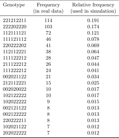
M = 9 and (3)n= 200,M = 30. For scenarios (1) and (2), we generate the genetic variableZi= (Zi1, . . . ,ZiM) based on the SLC17A1 gene (containing 9 SNPs) in the Clinical Antipsychotic Trails of Intervention Effectiveness (CATIE) study (Lieberman et al. (2005), Sullivan et al. (2008), Yolken et al. (2011)), the frequency distribution is shown in Table 2.1. We only take genotypes with≥7 (1% of sample size in data example, n= 690) occurrences in the real data for this simulation study. In scenario (3), we add 21 nuisance SNPs, each taking value 0, 1 or 2 with probability 0.3, 0.5 and 0.2, respectively.

Table 2.1: Frequency of genotypes used in the simulation study.

Genotype Frequency Relative frequency (in real data) (used in simulation)

221212211 114 0.191

222202220 103 0.174

112111121 72 0.121

111121112 46 0.078

220222202 41 0.069

112112221 38 0.064

111122212 28 0.047

211122212 26 0.044

111222212 24 0.041

002021122 21 0.034

212112221 15 0.025

002020022 10 0.017

102122222 10 0.017

102022222 9 0.015

002121122 8 0.013

002122222 8 0.013

220222211 8 0.013

102021122 7 0.012

202022222 7 0.012

For both estimation and testing simulations, we consider three choices of Σtrue:

Σtrue,1=



 

0.95 0.07 0.23 0.07 0.86 0.24 0.23 0.24 0.89





,Σtrue,2 =



 

0.95 0 0.

0 0.86 0

0 0 0.89





,Σtrue,2=



 

0.95 0 0.

0 0.86 0

0 0 0.89



(33)

The first covariance matrixΣtrue,1 is the estimated covariance matrix from the CATIE data

under the assumption that there is no SNP effect. The second choice,Σtrue,2, is a matrix that

is expanded by the diagonal elements ofΣtrue,1 and will be used to evaluate the performance of

our procedure where the outcomes are actually independent.Σtrue,3 introduces high correlation

betweenY1 and (Y2, Y3) and is used to demonstrate the effect of correlation on the performance of our procedure. When fitting the model, we first fit a working independence model and estimate Σ using residual covariance matrix, and then use the estimated Σ as the working covariance matrix in the joint estimation and testing procedures.

2.4.1 Estimation

In the simulation to evaluate our estimation procedure, we useh1(·) =z1+z2+z3+z1z4z5−z6/3− z7z8/2 + (1−z9),h2(·) =z1z2+z5(z7+z3) +z2z9,h3(·) =z2+z3+ (1−z6)2/3−z₅2/2 +z₈2−z₁2/3 forh for scenarios (1)-(3). For each of the scenarios, we generate 1000 data sets.

To evaluate the accuracy of the parameter estimates of β`, we investigate the empirical bias (Bias), empirical standard deviation (sd), estimated standard errors averaged over 1000 simulations (se) and coverage probabilities (Coverage) of 95% confidence intervals. The results are presented in Table 2.2. The original values are all multiplied by 100 and rounded to their 2-nd decimal places. From the table, we can see that, for all the cases, the biases are quite small and are negligible, estimated standard errors of β’s are very close to the empirical standard deviations, and the empirical coverage is close to the nominal level of 95%. As the sample size increases from 100 to 200, the bias decreases and the coverage increases slightly. The results suggest that our proposed method provides accurate estimate of β`, the coefficient of the covariates.

To measure the accuracy of the estimate ofh, we report the following evaluating criteria for each responses (`= 1,2,3)

M1` = n−1 n

X

i=1

{bh_`(Z_i)−h_`(Z_i)}2

M2` = n−1 n

X

i=1

|bh_`(Z_i)−h_`(Z_i)|.

The results are reported in the Table 2.3, together with the correlation between the predicted and the true Y’s. To evaluate the accuracy of our estimation for h(·), we fitbh_` onto h_` for all

three cases of Σtrue and ` = 1,2,3. Our ideal model of regressing bh’s onto the h’s would be

b

(34)

the estimate ofh(·) in the table:M1 andM2, which indicates high accuracy of the estimates of h(·). In addition, the results in the table also show high correlation between the predicted and the true value ofY for all settings, which indicates that our method performs well in predicting the responses.

In order to demonstrate the advantage of applying multivariate regression, we generate 100 datasets for combination of (n = 200, m = 9) under different settings of correlation between responses and compute the ratio of estimated standard error (SE) of h(·) for UVKM versus MVKM. Ratio is calculated as SE(hUVKM)/SE(hMVKM). Besides the cases when Σ = I3 and

Σtrue,3, we also compare the case when

Σ=Σtrue,4 =



 

1 0.8 0.6 0.8 1 0.8 0.6 0.8 1





.

(35)

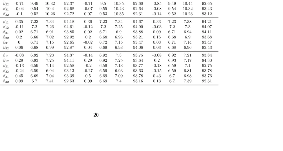
Table 2.2: Estimation ofβ’s for simulation study in Section 2.4. We report the empirical bias (Bias), empirical standard deviation (sd), estimated standard errors averaged over 1000 simulations (se) and coverage probabilities (Coverage) of 95% confidence intervals. The biases are calculated from comparing the estimated values with the true values of β’s, (0.7,1),(0.7,1),(0.7,1). The original values are multiplied by 100 and rounded to their 2nd decimal places.

Σ1 Σ2 Σ3

(n, m) Bias sd se Coverage Bias sd se Coverage Bias sd se Coverage

(100,9)

β11 -0.26 10.2 10.72 93.17 -0.27 10.2 10.77 92.71 -0.13 10.2 10.84 92.80

β12 -0.67 10.18 10.69 93.62 -0.66 10.18 10.7 93.63 -0.82 10.18 10.88 93.23

β21 0.39 9.52 10.55 92.41 0.42 9.53 10.52 92.69 0.31 9.51 10.58 91.90

β22 -0.71 9.49 10.32 92.37 -0.71 9.5 10.35 92.60 -0.85 9.49 10.44 92.65

β31 -0.04 9.54 10.4 92.68 -0.07 9.55 10.43 92.64 -0.08 9.54 10.32 93.43

β32 -0.1 9.52 10.26 92.72 0.07 9.53 10.35 92.31 -0.14 9.52 10.23 93.12

(200,9)

β11 0.35 7.23 7.34 94.18 0.36 7.23 7.34 94.67 0.33 7.23 7.38 94.21

β12 -0.11 7.2 7.26 94.61 -0.12 7.2 7.25 94.90 -0.03 7.2 7.3 94.07

β21 0.02 6.71 6.91 93.85 0.02 6.71 6.9 93.88 0.09 6.71 6.94 94.11

β22 0.2 6.68 7.02 92.92 0.2 6.68 6.95 93.21 0.15 6.68 6.9 93.68

β31 0 6.71 7.15 92.65 -0.02 6.72 7.15 93.47 0.03 6.71 7.14 93.47

β32 0.06 6.68 6.99 92.87 0.04 6.69 6.93 94.06 0.03 6.68 6.96 93.43

(200,30)

β11 -0.08 6.92 7.23 94.37 -0.14 6.92 7.3 93.75 -0.08 6.92 7.21 93.84

β12 0.29 6.93 7.25 94.11 0.29 6.92 7.25 93.64 0.2 6.93 7.17 94.30

β21 -0.13 6.59 7.14 92.58 -0.2 6.59 7.13 93.77 -0.18 6.59 7.1 92.75

β22 -0.24 6.59 6.94 93.13 -0.27 6.59 6.93 93.63 -0.15 6.59 6.81 93.78

β31 0.45 6.69 7.04 93.39 0.5 6.69 7.09 93.78 0.43 6.7 6.98 93.76

(36)

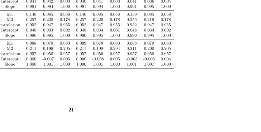
Table 2.3: Model Evaluation for measure the accuracy of the estimate of h. Displayed are the two M’s defined in Section 2.4, the correlation between the estimated Y and its true value, and the slope and intercept of fitting the simple linear model bh=h.

Σ1 Σ2 Σ3

(n, m) k= 1 k= 2 k= 3 k= 1 k= 2 k= 3 k= 1 k= 2 k= 3

(100, 9)

M1 0.186 0.137 0.113 0.186 0.137 0.114 0.186 0.137 0.113 M2 0.307 0.276 0.249 0.308 0.276 0.249 0.307 0.276 0.248 correlation 0.955 0.950 0.958 0.955 0.950 0.958 0.955 0.950 0.958 Intercept 0.041 0.042 0.003 0.040 0.041 0.003 0.041 0.036 0.004 Slope 0.991 0.994 1.000 0.991 0.994 1.000 0.991 0.995 1.000

(200, 9)

M1 0.140 0.085 0.058 0.140 0.085 0.058 0.139 0.085 0.058 M2 0.257 0.220 0.178 0.257 0.220 0.178 0.256 0.219 0.178 correlation 0.952 0.947 0.955 0.952 0.947 0.955 0.952 0.947 0.955 Intercept 0.048 0.033 0.002 0.048 0.034 0.001 0.048 0.034 0.002 Slope 0.990 0.995 1.000 0.990 0.995 1.000 0.990 0.995 1.000

(200, 30)

(37)

Index of genotypes

Ratio

1 3 5 7 9 11 13 15 17 19

1.00

1.05

1.10

1.15

1.20

Index of genotypes

Ratio

1 3 5 7 9 11 13 15 17 19

1.00

1.05

1.10

1.15

1.20

Index of genotypes

Ratio

1 3 5 7 9 11 13 15 17 19

1.00

1.05

1.10

1.15

1.20

Index of genotypes

Ratio

1 3 5 7 9 11 13 15 17 19

1.00

1.05

1.10

1.15

1.20

Index of genotypes

Ratio

1 3 5 7 9 11 13 15 17 19

1.00

1.05

1.10

1.15

1.20

Index of genotypes

Ratio

1 3 5 7 9 11 13 15 17 19

1.00

1.05

1.10

1.15

1.20

Index of genotypes

Ratio

1 3 5 7 9 11 13 15 17 19

1.00

1.05

1.10

1.15

1.20

Index of genotypes

Ratio

1 3 5 7 9 11 13 15 17 19

1.00

1.05

1.10

1.15

1.20

Index of genotypes

Ratio

1 3 5 7 9 11 13 15 17 19

1.00

1.05

1.10

1.15

1.20

Figure 2.1: The figure compares the precision of estimation between UVKM and MVKM under different correlation settings. The Y axis is the ratio of standard error achieved by applying these two methods (as defined in Section 2.4). The x axis indicates all the genotypes shown in Table 2.1. The correlation between responses are Σ = I3 (left), Σ =

(38)

2.4.2 Testing

To evaluate our testing procedure, we consider the following choices of the functions: (a)h1= h2 =h3= 0, (b)h1 =δ(z1+z2+z3+z1z4z5−z6/3−z7z8/2+(1−z9)) forδ= 0.02,0.04, . . . ,0.18;

h2 = h3 = 0. (c) h1 = δ(z1 +z2 +z3 +z1z4z5 −z6/3−z7z8/2 + (1−z9)), h2 = δ(z1z2 +

z5(z7 +z3) +z2z9) for δ = 0.02,0.04, . . . ,0.18; h3 = 0. Scenario (a) corresponds to Type I

error of our procedure, and scenario (b) and (c) are used to compute power as the genetic effect deviates from the null hypotheses with increasing values of δ for p0 = 1 and p0 = 2, respectively. For each combination of (n, m) described in scenarios (1)-(3), we investigate the performance of our test with p0 = 1 andp0 = 2. We also compare our test with the standard univariate kernel machine (UVKM) test forp0= 1 and with Bonferroni corrected UVKM tests for p0 = 2. Significance level α = 0.05 is used in all the testing procedures. The proportions

of rejections are recorded and shown in Table 2.4 and Table 2.5. From Table 2.4, we can see that the Type I errors are controlled around 0.05 for both of the methods, but UVKM test with Bonferroni correction is more conservative. Comparing with UVKM test, MVKM has slightly improved power, because this is the case when testing for a single function and MVKM test is not expected to have pronounced difference in performance. Table 2.5 shows the results when testing for twoh(·) functions, where MVKM outperforms UVKM test for all the settings, especially when the correlations are high between the responses (Σ3). This results suggest that

(39)

Table 2.4: Simulation results for testing for one h function. Displayed are the power of our test (MVKM) along with multiple univariate testing with Bonferroni correction (UVKM) for different settings (α= 0.05).

(n, m) δ= 0 δ= 0.02 δ= 0.04 δ= 0.06 δ= 0.08 δ= 0.1 δ= 0.12 δ= 0.14 δ= 0.16 δ= 0.18

(100,9) Σ1

MVKM 0.055 0.099 0.183 0.41 0.477 0.685 0.852 0.94 0.982 0.994

UVKM 0.050 0.083 0.156 0.395 0.401 0.625 0.791 0.91 0.959 0.99

Σ2

MVKM 0.057 0.081 0.166 0.298 0.491 0.701 0.873 0.944 0.983 0.994

UVKM 0.049 0.076 0.145 0.262 0.417 0.626 0.8 0.911 0.96 0.991

Σ3

MVKM 0.051 0.078 0.135 0.286 0.43 0.632 0.789 0.916 0.968 0.991

UVKM 0.044 0.06 0.102 0.26 0.381 0.592 0.746 0.881 0.947 0.98

(200,9) Σ1

MVKM 0.052 0.11 0.309 0.562 0.845 0.963 0.996 1 1 1

UVKM 0.050 0.105 0.283 0.499 0.784 0.945 0.99 1 1 1

Σ2

MVKM 0.051 0.096 0.263 0.571 0.841 0.967 0.998 1 1 1

UVKM 0.052 0.087 0.241 0.481 0.765 0.935 0.994 0.999 1 1

Σ3

MVKM 0.051 0.092 0.229 0.516 0.789 0.942 0.994 1 1 1

UVKM 0.047 0.088 0.219 0.45 0.72 0.909 0.982 0.999 1 1

(200,30) Σ1

MVKM 0.052 0.079 0.203 0.45 0.73 0.924 0.993 0.999 1 1

UVKM 0.047 0.08 0.178 0.386 0.659 0.887 0.978 0.999 0.999 0.999

Σ2

MVKM 0.054 0.09 0.208 0.477 0.762 0.946 0.994 0.999 1 1

UVKM 0.050 0.07 0.178 0.393 0.657 0.892 0.979 0.999 0.999 1

Σ3

MVKM 0.060 0.086 0.2 0.412 0.697 0.888 0.975 0.995 0.999 1

(40)

Table 2.5: Simulation results for testing for two h functions. Displayed are the power of our test (MVKM) along with multiple univariate testing with Bonferroni correction (UVKM) and Type I errors (δ= 0) for different scenarios (α= 0.05).

(n, m) δ= 0 δ= 0.02 δ= 0.04 δ= 0.06 δ= 0.08 δ= 0.1 δ= 0.12 δ= 0.14 δ= 0.16 δ= 0.18

(100,9) Σ1

MVKM 0.056 0.098 0.181 0.41 0.476 0.687 0.856 0.941 0.982 0.994

UVKM 0.048 0.082 0.154 0.394 0.4 0.626 0.793 0.911 0.959 0.99

Σ2

MVKM 0.058 0.08 0.164 0.298 0.49 0.704 0.876 0.945 0.983 0.994

UVKM 0.049 0.076 0.143 0.261 0.414 0.627 0.801 0.912 0.96 0.991

Σ3

MVKM 0.055 0.077 0.134 0.286 0.432 0.635 0.792 0.916 0.968 0.991

UVKM 0.044 0.059 0.1 0.258 0.38 0.591 0.747 0.879 0.947 0.98

(200,9) Σ1

MVKM 0.052 0.112 0.308 0.564 0.849 0.963 0.996 1 1 1

UVKM 0.05 0.106 0.285 0.502 0.787 0.945 0.99 1 1 1

Σ2

MVKM 0.052 0.098 0.263 0.577 0.846 0.967 0.998 1 1 1

UVKM 0.053 0.089 0.243 0.485 0.769 0.933 0.994 0.999 1 1

Σ3

MVKM 0.051 0.093 0.228 0.522 0.791 0.94 0.994 1 1 1

UVKM 0.046 0.09 0.221 0.452 0.721 0.905 0.982 0.999 1 1

(200,30) Σ1

MVKM 0.052 0.08 0.206 0.451 0.732 0.926 0.993 0.999 1 1

UVKM 0.046 0.079 0.182 0.388 0.662 0.888 0.978 0.999 0.999 0.999

Σ2

MVKM 0.054 0.09 0.209 0.479 0.764 0.949 0.994 0.999 1 1

UVKM 0.049 0.069 0.179 0.396 0.658 0.893 0.979 0.999 0.999 1

Σ3

MVKM 0.06 0.087 0.202 0.412 0.698 0.89 0.977 0.995 0.999 1

(41)

2.5 Data Analysis

To demonstrate the usefulness of our proposed methods, we apply the methodology to a dataset that consists of 520 Epstein-Barr virus (EBV) immortalized LCLs from unrelated Caucasian participants of the CAP clinical trials.

Pharmacogenomics is the study of the variability in drug response which is due to underlying individual variation in genetic architecture, and drug response can include drug efficacy, adverse drug reactions or drug toxicity. Comparing with common disease association studies, identified associations in pharmacogenomics can immediately be useful to patients and physicians in a clinic. For example, if genetic associations are identified for prediction the proper dose of a medication, a physician can use the genotype information of a patient as a guide to their dosing (Ritchie (2012)).

Even though pharmacogenomics studies have produced promising discoveries, there are lim-itations in identifications and validation of genetic markers. In practice, it is often the case that several genetic variations jointly contribute to a phenotype of drug response, which requires a relatively large sample size to detect. However, many pharmacogenomic traits and drug re-sponses have very limited sample size. One extreme case is that drugs that exist life-threatening adverse effect will be removed from the market. Most pharmacogenomic studies are amended to existing clinic trials, which confines the researchers in terms of the experimental design. More-over, it is often the case that the study can not be designed in an optimal way for genetic or genomic research. For example, it is unethical to have a group of patients who are not provided with a drug, especially if the drug is FDA approved with benefits to patients. Controlling po-tential confounding factors, such as comorbidities, dosing and diet, adds another complication to pharmocogenomics study using clinical trials.

Because of these the limitations and issues, in vitro study designs using human cell-based models have been proposed and developed for pharmocogenomics discovery. In these experi-ments, cell lines are perturbed with drug treatment and changes in gene expression and cell growth in response to drugs can be observed. Unlike clinical trials, which requires large number of patients to obtain reliable data and are expensive and time-consuming, cell-based models can generate large number of samples in a cost-effective manner. However, the number of choices of cell types for cell-based models is limited. An ideal cell type should have the following two characteristics: Firstly, the tissue is easy to access and inexpensive to obtain. Secondly, the drug response pathways are active within the tissue. Red blood cells or lymphocytes have proven to be very successful alternatives.

(42)

transforma-tion of human lymphocytes by EBV (a human herpesvirus that can infect human B lymphocytes and drives the cells into a permanent proliferation). It is relatively simple to isolate lympho-cytes, which can be obtained from small volumes of blood samples (Ling and Huls (2005)). In the procedure of generating LCLs, lymphocyte cells are separated from whole blood using density centrifugation, then the transformation of B lymphocytes is caused by the infection of EBV, and lastly, T cells are removed from the population.

The majority of pharmacogenomic studies in the LCL model have focused on the genetic association with chemotherapeutic susceptibility. Most chemotherapeutic agents produce a cy-totoxic effect in immortalized cell lines, and thus, measuring a pharmacogenomic phenotype in LCLs is straightforward. The data in our analysis measures the cytotoxic responses of 29 anticancer agents using LCLs model, which consists of 520 EBV imortalized LCLs that are derived from unrelated Caucasian participants of the CAP clinical trail (Medina et al. (2008), Brown et al. (2014)). In the experiment, each cell line was seeded on two 384-well plates, which contains 4000 cells for each well. 14 anticancer drugs were applied to the first plate and 15 to the second, and each LCL was exposed to six different concentrations for each drug. The drug responses for all the drugs were assessed using alamarBlue (Biosource International, CA, USA) by assuming that the raw fluorescence units are proportional to the concentration of living cells in each well. The responses were then normalized based on a lethal dose of 10% dimethyl sul-foxide (DMSO) and 0.1 % DMSO, as described in detail in Brown et al. (2011). In our analysis, we study the association between cytotoxic response to temozolomide and genetic variations on chromosome 10 using data generated from the LCLs study.

Though LCLs model has its benefits in various ways, there exist many opportunities for non-genetic factors to be introduced in the path from human donor to the study of an LCL in vitro, such as random selection of subpopulation of lymphocytes, temperatures, culture me-dia, etc.. In addition, since many chemotherapeutic drugs are designed to control the rapid growth of cells, correlation between cell growth rate and sensitivity to chemotherapeutic drugs is expected. LCL growth rate has been shown to be associated with chemotherapeutic-induced cytotoxicity and should be considered in all LCL analyses (Choy et al. (2008)). Therefore, in our real data analysis, we consider temperature, growth rate and experimental batch as our non-genetic covariates. Furthermore, principal component analysis (PCA) was applied to assess the possibility for substructure when conducting quality control over the genetic data in the LCLs study and the first two PCs were significant, so these PCs are also considered in the association study.

To understand the association between cytotoxic response to temozolomide and genetic variations on chromosome 10, we consider the model in our analysis, for i = 1, . . . ,520 and

`= 1, . . . ,6,