| INVESTIGATION
Estimation of Gene Insertion/Deletion Rates
with Missing Data
Utkarsh J. Dang,*,1Alison M. Devault,†Tatum D. Mortimer,‡Caitlin S. Pepperell,‡Hendrik N. Poinar,§ and G. Brian Golding**,2 *Departments of Biology and Mathematics and Statistics, McMaster University, Hamilton, Ontario L8S-4L8, Canada,†MYcroarray, Ann Arbor, Michigan 48105,‡Departments of Medicine and Medical Microbiology and Immunology, School of Medicine and Public Health, University of Wisconsin, Madison, Wisconsin 53705, and§Department of Anthropology and **Department of Biology, McMaster University, Hamilton, Ontario L8S-4K1, Canada
ABSTRACTLateral gene transfer is an important mechanism for evolution among bacteria. Here, genome-wide gene insertion and deletion rates are modeled in a maximum-likelihood framework with the additionalflexibility of modeling potential missing data. The performance of the models is illustrated using simulations and a data set on gene family phyletic patterns fromGardnerella vaginalis
that includes an ancient taxon. A novel application involving pseudogenization/genome reduction magnitudes is also illustrated, using gene family data fromMycobacteriumspp. Finally, an R package calledindelmissis available from the Comprehensive R Archive Network athttps://cran.r-project.org/package=indelmiss, with support documentation and examples.
KEYWORDSgene insertion/deletion; indel rates; maximum likelihood; unobserved data
L
ATERAL gene transfer is an important, yet traditionally underestimated, mechanism for microbial evolution (McDaniel et al.2010; Treangen and Rocha 2011). Whole gene insertions/deletions, referred to as indels here in the context of lateral gene transfer, can be deduced from exam-ining gene presence/absence patterns on a phylogenetic tree of closely related taxa. Systematic investigation of the rates of such indels can be done via several methods. Parsimony methods can be used (Hao and Golding 2004); however, these are known to underestimate the number of events in phylogeny reconstruction (Felsenstein 2004). Sequence characteristics such as codon usage bias and G+C content have also been investigated in the past, but these are not always reliable (Koski and Golding 2001). Alternatively, phy-logenies can also be constructed for individual genes, and a comparison of trees among individual genes can yield in-sights on the acquisition of foreign genes.Maximum-likelihood techniques have previously been used to estimate gene indel rates (Hao and Golding 2006;
Marri et al. 2006; Cohen and Pupko 2010). Traditionally, such likelihood-based analyses have required that the closely related sequences being investigated have complete genome sequences available. This ensures that no genome rearrange-ment masks a homolog (Hao and Golding 2006). Here, likelihood-based models are investigated that can also account for potentially unobserved or missing data.
The term“missing”here is used in a loose and informal sense. It is meant to measure the degree to which unobserved data may nevertheless contribute to a taxon’s data set, given the inferred rates from related taxa. Two different kinds of missing data are used here for illustration purposes.
In thefirst example, consider a taxon or a few taxa that have only subsets of their genome sampled. This could be due to genome degradation, errors in sequencing, errors in assembly, or incomplete next generation sequencing (NGS) studies. In bacterial evolution, genes are continually being inserted or deleted and the goal here is to estimate how much of the data has been missed within this background of continuous gene insertion/deletion.
As a second example, consider an intracellular pathogenic bacteria. It is well known that such species will adapt to their host by deleting unnecessary genes. Here, the missing data allude to the magnitude of genome reduction beyond the normal levels of genome flux. The goal, in this case, is to estimate this reduction while simultaneously estimating Copyright © 2016 by the Genetics Society of America
doi: 10.1534/genetics.116.191973
Manuscript received May 24, 2016; accepted for publication August 17, 2016; published Early Online August 25, 2016.
1Present address: Department of Mathematical Sciences, Binghamton University, State University of New York, Binghamton, NY 13902.
phylogenetic insertion/deletion rates. Not accounting for these missing data will bias estimates of indel rates.
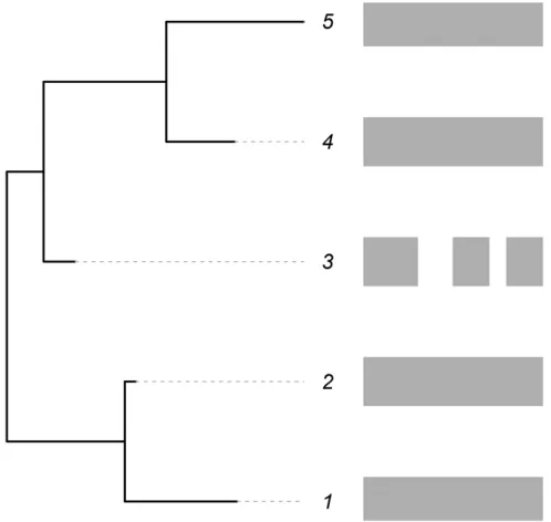
As an illustration, see Figure 1. Here, sequences for coding genes (shaded rectangles) are available forfive closely related taxa. Unexpectedly, the data available for the third taxon seem to differ from those for the other taxa, and this taxon appears to be missing some genes that are present in the others. If these are closely related taxa, they should have approximately similar amounts of coding information. Hence, the data recorded for the third taxon seem to be unusual in comparison to related taxa. Indeed, it seems that more deletion has occurred in this taxon relative to the others. In this case, assuming that the third taxon has missing data as discussed above (via either of the two scenarios), modeling of the insertion and deletion rates for genes for all five of the taxa directly would lead to an over-estimate of the deletion rate for the entire clade. However, accounting for this unexpected event would provide better es-timates for the insertion/deletion rates and at the same time give an estimate of the proportion of missing data. Such a methodology would permit the separation of the confounded effects of missing data from normal gene gain and loss over time. The method cannot determine the reason that the data are missing but can estimate the magnitude. Note that while methods exist for handling missing data, ambiguous states, and sequencing error for nucleotides (Felsenstein 2004; Kuhner and McGill 2014; Yang 2014), this article is thefirst to propose dealing with missing data using such models on gene family membership data and to illustrate their performance.
As evolutionary rates can vary among different clades or lineages on a tree, the analyses presented also include results
from models that relax the assumption of homogeneity of gene insertion and deletion rates across all branches on the phylogeny. Such models can yield unique estimates of in-sertion and deletion rates for specific clades (or branch and node groupings) chosen based on evolutionary time or prior in-formation. An R package called indelmiss (insertiondeletion analysis while accounting formissing data) is provided that allows for efficientfitting of all models discussed (Appendix D). The rest of this article is structured as follows.Materials and Methods includes details on the likelihood calculations and the formulation of a model that incorporates missing data. Results illustrates model performance using simulations and data based on gene phyletic patterns fromGardnerella vaginalis andMycobacteriumspp. Finally, some conclusions and ideas for future work are discussed in theDiscussionsection.
Materials and Methods
To model gene evolution, a two-state (presence or absence) continuous-time Markov chain is used. Genes are assumed to be inserted or deleted independently of other genes and at constant rates. To eliminate the problem of paralogs, only the presence or absence of gene families is considered in the fashion of Hao and Golding (2004, 2006). Any paralogs are clustered as a single gene family and only one member of a family is retained. The criteria for being considered as be-longing to a gene family are given inResults. For the Markov chain, an operational taxonomic unit (OTU) having a gene family present or absent is represented by a 1 or a 0.
Let the instantaneous rates of insertion and deletion ben andm;respectively. Then, the rate matrixQcan be written as
2m m
n 2n
; where the rows (and columns) represent
presence and absence in the current (future) state, respec-tively. The transition rate matrix representing the probabili-ties of a transition from one state to the next can be easily derived (cf. Hao and Golding 2006),
1
mþn3
nþmexpð2ðmþnÞtÞ m2mexpð2ðmþnÞtÞ
n2nexpð2ðmþnÞtÞ mþnexpð2ðmþnÞtÞ
;
where, as for Q; the rows (and columns) represent presence and absence in the current (future) state, respec-tively. For example, the probability of gene pres-ence in a descendant OTU ðPdÞ given that it was also present in the ancestral OTU ðPaÞ is given here by pðPdjPa;tÞ ¼pPaPd¼ ðmþnÞ
213ð
nþmexpð2ðmþnÞtÞÞ: Figure 1 An illustration of the scenarios being modeled. The shaded bars
on the right indicate gene content (presence/absence) within the ge-nomes offive species related according to the phylogeny given on the left. The third species is missing some gene blocks that are present in the other species.
Table 1 The proportionðdiÞof data that is unexpectedly missing in
the data for species i compared to closely related taxa on the phylogenetic tree
Observed
True “0” “1”
“0” 1 0
Hence, the values ofnandmmeasure the rate of gene inser-tions (deleinser-tions) per gene family. This method requires a known phylogenetic tree to be provided as it is not designed to generate a tree. It is also possible to have different indel rates assigned to different parts of the phylogenetic tree if desired.
Evaluating the likelihood on a given phylogenetic tree is straightforward (Felsenstein 1973, 1981). As in Yang (2014), LiðgiÞis defined as the conditional probability of observing data at the tips that are descendants of nodei, given that the state at nodeiisgi:Here,gican be either gene presence (P) or absence (A). Traditionally, LðiÞðgiÞ ¼1 if gi is observed at
node iand 0 otherwise. However, LðiÞ are not restricted to sum to one because they are not probabilities of different outcomes but rather probabilities of the same observation conditional on different events (Felsenstein 2004). Here, the “missingness” of the data is accommodated using this definition. If a gene is recorded as absent at tipi, the vector of conditional probabilities isLðiÞðAÞ ¼ ðd;1Þ9;i.e., the
prob-ability of observing gene absence given a gene is truly present (absent) is d ð1Þ: In effect, without such a correction, the conditional probability of observing gene presence given true gene presence is being underestimated. Similarly, if a gene is recorded as present at tipi, the vector of conditional proba-bilities isLðiÞðPÞ ¼ ð12
d;0Þ9;i.e., the probability of observing gene presence given a gene is truly present (absent) is 12dð0Þ: Here,dis the proportion of data that is unexpectedly missing compared to closely related taxa on the phylogenetic tree. Extending this formulation to multiple taxa, a vector of miss-ing proportions can be constructed asd¼ ðd1;. . .;dsÞ9fors number of taxa, where d2 ½0;1: Table 1 summarizes the corrections necessary for the conditional probabilities.
Then, for a nodeiwith two daughter nodesjandktimestj andtkapart, respectively,
LiðgiÞ ¼
" X
gj
pgigjðtjÞLjðgjÞ
# 3
" X
gk
pgigkðtkÞLkðgkÞ
# :
This conditional probability vector can be calculated for each node in the tree in a postorder tree traversal fashion. Finally, the probability vector is weighted by the root probabilityðpx0Þ of the states at the root of the tree. This yields the probability of the observedhth gene family presence/absence data given the tree as
fðxhÞ ¼
X
x0
px0L0ðx0Þ :
The log-likelihood for then observed gene family patterns can then be calculated as lðQÞ ¼PNh¼1logðfðxhjQÞÞ: Typi-cally, when the same rates are being fitted to the entire tree (homogeneous rates), stationarity is assumed. How-ever, the probability of the observed gene family presence can also be estimated at the root within the maximum-likelihood framework. This improves thefit if the process of gain and loss has not reached stationarity (Spencer and Sangaralingam 2009).
However, genes that are not observed as present in any of the taxa,e.g., ancient genes that have been lost, are obviously omitted in the data. This reflects the sampling bias. A correc-tion for the sampling bias (Felsenstein 1992; Lewis 2001; Hao and Golding 2006; Cohen and Pupko 2010) can be im-posed such that the probability is conditional on observing the gene in at least one species,
Lhþ¼ L
h
12Lh 2;
whereLh
2is the probability of genehbeing absent in all taxa. Here,Lh
2;computed by calculating likelihood on the tree of interest using a vector of zeros as observed data, is the same for all genes.
Certain assumptions are made here that can be relaxed in future work. First, genes can be regained after having been deleted. Note that removing this assumption did not improve the results in Hao and Golding (2006). Next, paralogues are excluded in the construction of gene families. Finally, it is assumed that each gene has an equal probability of not being recorded as present;i.e., the missingness is equally prevalent among different sites in the genome.
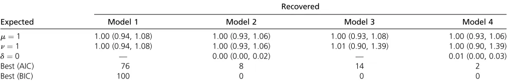
Four models are used for the analyses here. These four models estimate indel rates (where the deletion rate is the same as the insertion rate,i.e.,m¼n), indel rates with pro-portions of missing data for taxa of interestðdÞ;unique in-sertion and deletion rates, and unique inin-sertion and deletion rates with proportions of missing data for taxa of interest, respectively. These models are referred to as models 1–4 hereon. This is thefirst article to investigatefitting and esti-mating proportions of missing data (models 2 and 4) on gene Table 2 Mean estimates for indel rates and proportion of missing data along with the ranges across 100 runs for simulation set 1
Recovered
Expected Model 1 Model 2 Model 3 Model 4
m¼1 1.00 (0.94, 1.08) 1.00 (0.93, 1.06) 1.00 (0.93, 1.08) 1.00 (0.93, 1.06)
n¼1 1.00 (0.94, 1.08) 1.00 (0.93, 1.06) 1.01 (0.90, 1.39) 1.00 (0.90, 1.39)
d¼0 — 0.00 (0.00, 0.02) — 0.01 (0.00, 0.03)
Best (AIC) 76 8 14 2
Best (BIC) 100 0 0 0
family membership data. The models were implemented in R (R Core Team 2014) and are available as a package ( Appen-dix D). Parameter estimates and standard errors are obtained from numerical optimization, using PORT routines (Gay 1990) as implemented in the nlminbfunction in R and the hessian function in package numDeriv(Gilbert and Varadhan 2012), respectively.
Data availability
The authors state that all data necessary for confirming the conclusions presented in the article are represented fully within the article and the {\sf R} package available online.
Results
The likelihood-ratio test is known to favor parameter-rich models in large molecular data sets (Yang 2014, p. 146). However, choosing a best-fitted model from a set of models can be done conveniently with penalized likelihood-based model selection criteria. Here, we make use of both the Akaike information criterion (AIC) (Akaike 1973) and the Bayesian information criterion (BIC) (Schwarz 1978) to pick a model with superiorfit to the data,
BIC¼2lðQÞ^ 2logN3m
AIC¼2lðQ^Þ223m;
wherelðQ^Þis the log-likelihood at the maximum-likelihood estimates,Nis the number of gene phyletic patterns, andmis the number of parameters estimated for the model.
Simulations
Multiple simulations were conducted to evaluate parameter recovery and judge the efficacy of the model selection criteria.
Simulation set 1:One hundred random samples of 5000 gene presence/absence phyletic patterns were simulated for six taxa with m¼n¼1; using the phangorn package (Schliep 2011) in R. For simulating each sample, a tree was randomly generated using the APEpackage (Paradiset al. 2004) in R with the branch lengths sampled from a beta distribution with shape parameters 1 and 4 (to simulate closely related taxa). Here, missingness was not simulated. Models 1–4 were run on these. All models yielded insertion and deletion rate estimates close to generating values. A Kruskal–Wallis rank sum test for themestimates andn esti-mates from the four models yielded P-values of 0.645 and 0.781, respectively (note that ANOVA with a Welch correc-tion for homogeneity also does not yield enough evidence to reject the null). This implies that the modelsfitting a missing data proportion yielded rate estimates that were similar to the estimates from models 1 and 3. The BIC and AIC picked the generating model (model 1) 100 and 76 times, respec-tively. For models 2 and 4, a missing data parameter was fitted for the OTU at tip 1 in each of the 100 runs. Model 4, whichfitted insertion and deletion rates along with a missing
data proportion, yielded on averagem^¼0:998;^n¼1:003; and^d¼0:005 (median^d¼0:001) across the 100 runs (Ta-ble 2).
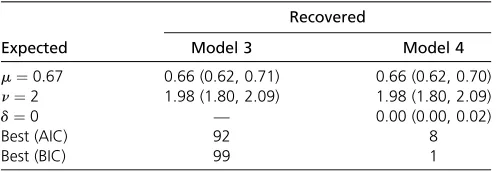
This simulation was repeated with unequal deletion and insertion rates: m¼0:67 and n¼2; respectively. Models 3 and 4 were run on these (Table 3). The BIC and AIC picked the generating model (model 3) 99 and 92 of 100 times, re-spectively. Both model 3 and model 4 yielded average esti-mates ofmandnthat were very close to the values used in the simulation. Model 4 estimated an average^d¼0:002 (for the OTU at tip 1) with a median^d¼0:000:Welch two-sample two-sidedt-tests (not assuming equal variance) comparingm andn estimates (from models 3 and 4) yieldedP-values of 0.476 and 0.824, respectively.
Again, this last simulation was repeated with unequal deletion and insertion rates: m¼0:67 and n¼2; respec-tively. But, after the phyletic patterns were generated, a pro-portion of genes that were originally present for a single taxon (tip 1; same across runs) were recorded as absent in each run. This proportion was sampled in each simulation from a uniform distribution between 0 and 0.6. Note that the upper limit of 0.6 is arbitrary and used for convenience; a higher upper limit could easily have been used. The BIC and AIC picked the generating model (model 4) 95 and 97 times, respectively (Table 4). As expected, the model selection cri-teria picked model 3 on those occasions where the estimated missing data proportion was very small and so model 4 did not result in a substantially betterfit to the data. Model 3, which cannot account for a missing data proportion, yielded an averagem^¼1:127 and^n¼2:765 across the 100 runs. On the other hand, model 4 averagedm^¼0:665;^n¼1:982;and d2^d¼0:001 for tip 1 (median^d¼0:000). Clearly, model 4 yields insertion and deletion rate estimates close to the gen-erating values while providing a reasonable estimate of the proportion of missing data. Table 4 also shows tighter ranges for the estimates for model 4 across the 100 runs. Welch two-sample two-sidedt-tests comparingm andnestimates (from models 3 and 4) yieldedp-values equal to 3:05931028and 1:97631024; respectively. A Welch two-sample one-sided
t-test comparing deletion rate estimates from models 3 and 4 suggests that model 3 yields, on average, a higher estimate for deletion rate than model 4 (p-value , 1:52931028). This supports our thesis that artificially inflated deletion Table 3 Mean estimates for indel rates and proportion of missing data along with the ranges across 100 runs for simulation set 1
Recovered
Expected Model 3 Model 4
m¼0:67 0.66 (0.62, 0.71) 0.66 (0.62, 0.70) n¼2 1.98 (1.80, 2.09) 1.98 (1.80, 2.09)
d¼0 — 0.00 (0.00, 0.02)
Best (AIC) 92 8
Best (BIC) 99 1
rates are inferred if missing data are not explicitly accounted for in these indel rate models.
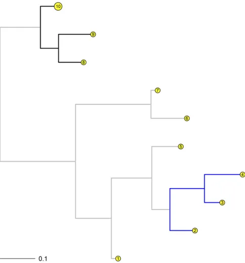
Simulation set 2:As noted in the Introduction, evolutionary rates can vary among different clades or lineages on a tree and so here, heterogeneous gene insertion and deletion rates among different lineages are simulated and analyzed in the presence of missing data. Five hundred random samples of 5000 gene presence/absence phyletic patterns were simu-lated for 10 taxa (Figure 2). First, a tree with 10 taxa was generated with branch lengths sampled from a beta distribu-tion with shape parameters 1 and 8 (to simulate closely re-lated taxa). The patterns simure-lated using the phangorn package were based on base deletion rates sampled from between 0.625 and 1.167 with the insertion rates exploring the interval between 0.875 and 2.500. The branch lengths for the clades with the branches in blue and black in Figure 2 were multiplied by scaling factors sampled independently from the interval½1;3;respectively. As a result, the deletion (insertion) rates for the blue clade over the 500 samples were generated from ½0:652;3:375 ð½0:925;7:275Þ: Simi-larly, the deletion (insertion) rates for the black clade over the 500 samples were generated from ½0:627;3:383 ð½0:875;7:154Þ: Missing data were simulated at tips f1;3;5;6;9gby randomly and independently sampling from a uniform distribution between 0 and 0.6. For the analy-ses, tips f1;2;3;5;6;8;9g were allowed a missing data proportion.
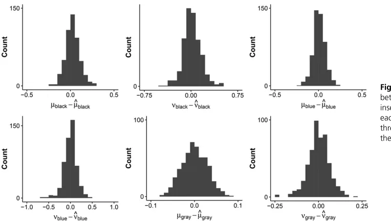
Model 4 was run on all 500 samples. Moreover, the prob-ability of gene family presence was also estimated at the root. Both models, with and without estimating the probability of gene family presence at the root, perform well on average. The parameter estimates are close to the sampled parameters. For example, for the model that did not estimate the probability of gene family presence at the root, the difference in given and estimated parameters for the unique insertion and deletion rates for the three colored clades centered on 0.009 (median 0.006) for the 500 samples (see Figure 3).
Moreover, the estimated proportions of missing data are also close to the given parameters (Table 5). A note of caution for the reader: If the same 500 random samples are fitted with a missing data proportion for the 10th tip (where 1000 genes are then recorded as absent during data
simula-tion) instead of the 9th tip, the overall estimates do not vary by much. However, if the same samples arefitted with miss-ing data proportions for all tips (1–10), the models become overparameterized and while the recovered parameter esti-mates are reasonable on average, parameter estiesti-mates can deviate wildly, especially for longer trees (seeDiscussion). In the context of accounting for sequence errors in nucleotide models, Yang (2014) recommends that at least one genome be free of sequence errors. Here, we err on the side of caution, and for the real data analyses, a minimum of three taxa are assumed to not possess any missing data and are modeled without missing data proportions.
InAppendix E, we test cases where only the lineages with the highest apparent gene data loss are modeled with a pro-portion of missing data. This is a type of model misspecifi ca-tion. Nevertheless, the results are reasonably good despite the inappropriateness of the test.
Two examples
G. vaginalis data: Data containing gene presence/absence measurements on 2036 genes for 35 OTUs of G. vaginalis (Figure 4) are analyzed.G. vaginalisis known to be associ-ated with bacterial vaginosis (Verhelstet al.2004; Menard et al.2008). One of these OTUs is a draft genome (labeled Troy), generated from the remains of a fossilized concretion from Troy, Western Anatolia (present-day Turkey). The tree was rooted on the branch leading toJCP7659, using Figtree (Rambaut 2014). These data yielded 746 distinct phyletic patterns of gene presence and absence. Of the total 2036 genes, 558 genes were present in all OTUs. But another Table 4 Mean estimates for indel rates and proportion of missing
data along with the ranges across 100 runs for simulation set 1
Recovered
Expected Model 3 Model 4
m¼0:67 1.13 (0.63, 5.09) 0.67 (0.62, 0.70) n¼2 2.77 (1.74, 14.72) 1.98 (1.80, 2.12)
d2^d¼0 — 0.00 (20:01;0.01)
Best (AIC) 97 3
Best (BIC) 95 5
For models 3 and 4, missing data were simulated for tip 1 (of six) with a random proportion sampled from a uniform distribution between 0 and 0.6. The last two rows give the number of times the AIC or the BIC selected the model in the column.
151 genes were present in all OTUs except the ancient ge-nomeTroy(seeAppendix A).
Method A: Models 1–4 werefitted to these gene phyletic patterns, assuming homogeneity of gene insertion and de-letion rates across all branches on the phylogeny. In addi-tion, for models 2 and 4, a missing data parameter wasfitted for all taxa except three (cf. Figure 4). The estimate for m¼n is 2:955ðSE¼0:067Þ: This implies that during the evolutionary time period required for one substitution per nucleotide site (on average), an entire gene could pos-sibly have been inserted/deleted three times. Model 2, which fits a proportion of missing data as well, yielded
^
m¼^n¼1:875ðSE¼0:052Þ:Clearly, estimating the propor-tion of missing data leads to a lower indel estimate. As in the simulations, this implies that not fitting a proportion of missing data explicitly can lead to artificially inflated indel estimates. Twenty-seven of the missing data proportions were estimated to be between 0 and 0.05, with four taxa between 0.05 and 0.1 and theTroystrain yielding an esti-mate of 0:248ðSE¼0:013Þ:Note that this model yielded superior AIC and BIC values to those of model 1. Moreover, the high missing data proportion for theTroystrain cannot be explained away by estimating unique insertion and de-letion rates as in model 3. This latter model yielded
^
m¼2:442ðSE¼0:065Þ and ^n¼3:760ðSE¼0:090Þ;
sug-gesting high rates of gene insertion and deletion; however, this model yielded inferior AIC and BIC values to those of model 2. This implies that accounting for possible missing data is more important to the model fit on these data than fitting deletion and insertion rates separately. Of all the models, model 4 results in the best fit to the data in terms of AIC ð243437:13Þ and BIC ð243628:18Þ values. After accounting for the missing data proportions,
^
m¼1:326ðSE¼0:046Þ and ^n¼2:577ðSE¼0:067Þ:
Fur-thermore, note that ^dTroy¼0:245ðSE¼0:013Þ; i.e., the missing data proportion for theTroystrain remained much
higher than expected (median estimated missing data pro-portion is 0.015). The insertion and deletion rates suggest that insertion is occurring at almost twice the rate of deletion after accounting for possible missing data. Accounting for the miss-ing data proportions dramatically reduces the estimate (close to half) for deletion rate between models 3 and 4.
Method B: Models 2 and 4 were also run assuming that all branches follow the same insertion and deletion rates but that the only taxon of interest with a missing data proportion is the Troy strain. This was done to check whether models 2 and 4 in method A were overparameterized and a simpler model could yield an equivalentfit. Similar results to those observed for method A were obtained. AIC and BIC values indicate that model 2 yields a superior fit to models 1 and 3 from method A. Estimates for ^dTroy from models 2 and 4 were 0:238 ðSE¼0:013Þ and 0:236ðSE¼0:013Þ; respectively. However, note that AIC and BIC values for method B models were consistently lower than for equivalent method A models.
between 0 and 0.05, with three taxa between 0.05 and 0.1 (ATCC14018, JCP7672, and A6420B all 0.063). The estimated missing data proportion for Troy was again 0:228ðSE¼0:013Þ; much higher than the median missing data proportion (0.015). The estimate of 0.228 corresponds to 273 genes. This supports Devault (2014) who noted, based on genome size comparisons, that the true gene con-tent of theG. vaginalis Troystrain may be underrepresented by between 200 and 300 genes. The clade with the Troy strain (green clade) has high estimated rates of inser-tion n^1¼10:536ðSE¼0:339Þ with an estimated rate of deletion m^1¼0:927ðSE¼0:158Þ after accounting for missing data proportions. Estimated rates of deletion and insertion for the red clade are m^2¼1:888ðSE¼0:305Þ and^n2¼7:001ðSE¼0:385Þ;respectively. The blue clade is found to have a low deletion rate ofm^3¼0:181ðSE¼0:031Þ with insertion rate estimated to ben^3¼1:781ðSE¼0:067Þ: The branches and the taxa connected by black colored branches, on the other hand, have a low estimated rate of insertion^n4 ¼0:906ðSE¼0:050Þwith an estimated rate of deletionm^4¼0:785ðSE¼0:047Þafter accounting for miss-ing data proportions. Moreover, the model selection criteria values suggest that the observed gene presence/absence data for Troy are not explained as well by a gene insertion/ deletion model without accounting for potential missing data. Other variations on the model variables in terms of clades or groups of branches with unique rates were also run (results not shown). However, model 4 from method C discussed above yielded the best fit in terms of AIC ð241;065:98Þ and BIC ð241;296:35Þ values among all models and methods.
Pathogenic bacteria data: The genus Mycobacterium in-cludes several causative agents of important diseases in hu-mans and animals. For example,Mycobacterium tuberculosis andM. lepraeare known to be the causative agents of tuber-culosis (Coleet al.1998) and leprosy (Coleet al.2001), re-spectively. M. ulcerans is known to cause Buruli ulcers in humans (Stinear et al.2007). M. bovis causes tuberculosis in cattle and M. avium causes disease in immunocompro-mised individuals (Senaratne and Dunphy 2009).
The Mycobacterium genus contains many intracellular bacteria. Among these,M. lepraeis a known obligate intra-cellular parasite. Most other species are facultative with the exception of the recently discoveredM. lepromatosisthat also causes leprosy (Hanet al.2009; Han and Silva 2014). Obli-gate intracellular bacteria are typically characterized by smaller genome sizes compared to facultative intracellular
or free-living bacteria (Bordenstein and Reznikoff 2005). Furthermore, close to half of the genome of M. leprae is known to be pseudogenes and noncoding regions (Cole et al. 2001). An analysis of gene insertion/deletion rates can shed light on rates of lateral gene transfer while provid-ing a maximum-likelihood estimate of how much codprovid-ing ge-netic material has been discarded (or become nonfunctional) given the passage of evolutionary time and the evolutionary relationships between congenericMycobacteriumspecies.
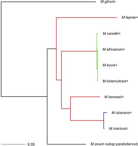
To identify gene families, a procedure similar to that of Hao and Golding (2004, 2006) was followed. This procedure was applied to 10 congeneric Mycobacterium genomes down-loaded from the NCBI as outlined inAppendix B. A phylogeny forMycobacteriumspecies has been proposed in the literature (O’Neillet al.2015). Details on the construction of the phy-logenetic tree are provided in the above-mentioned article. Here, we use a pruned version of the tree (Figure 5) from O’Neill et al.(2015) and analyze the gene family presen-ce/absence data as outlined inAppendix B. Note that theM. lepraegenome used in the construction of their tree was dif-ferent: O’Neillet al.(2015) usedM. leprae Br4923with ac-cession no. NC_011896.1 while we used M. leprae TN (NC_002677.1) (Appendix C).
Models 1–4 werefitted to the gene phyletic patterns given the tree constructed above, assuming homogeneity of gene insertion and deletion rates across all branches on the phy-logeny (method A). Missing data proportions werefitted for all taxa except three (cf. Figure 5). Note that as seen for theG. vaginalis analysis, models 2 and 4fitted the data better in terms of AIC and BIC values compared to models 1 and 3, respectively. High missing data proportions were estimated forM. lepraeandM. ulceranscompared to the median missing data proportions of 0.034 and 0.036 from models 2 and 4, respectively. Model 4, whichfits both insertion and deletion rates, yielded estimates of ^dM: leprae¼0:500ðSE¼0:011Þ and^dM: ulcerans¼0:242ðSE¼0:007Þ:The high missing data proportion estimate forM. lepraeis in line withfindings of an extreme case of reductive evolution (Coleet al.2001; Gómez-Valeroet al.2007).
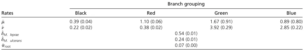
The assumption of homogeneous indel rates across all branches was relaxed and different models werefitted accord-ing to different combinations of clades or branch groupaccord-ings with unique indel rates. In terms of AIC and BIC values, model 4 with unique rates for each of the colored branches in Figure 5 fitted the best (method B; Table 7). For the best-fitting model, the probability of gene family presence at the root was also estimated (i.e., we do not assume that stationarity has been achieved), which improved thefit of the model. The Table 5 Ranges for differences between simulated and estimated proportion of missing data for the corresponding taxa over 500 samples from simulation data set 2
Tip labels
Difference 1 2 3 5 6 8 9
probability of gene family presence at the root was estimated to be 0.066 (SE = 0.004). Using this model, missing data proportions estimated for M. leprae and M. ulcerans are 0:543ðSE¼0:011Þ and 0:239ðSE¼0:009Þ (median esti-mated missing data proportion is 0.024), corresponding to 1660 and 869 genes, respectively.
The branches in red in Figure 5 had an estimated rate of deletion m^1¼1:097ðSE¼0:061Þ and estimated rate of in-sertion ^n1¼0:379 ðSE¼0:024Þ:The low rate of insertion and relatively low rate of deletion (high compared to the rate of insertion) corresponds well withM. leprae being a niche specialist. Indeed, a recent study found remarkable genomic conservation and that very few large insertions or deletions have taken place in a comparison of ancient and modern M. leprae strains (Schuenemann et al. 2013). Moreover, note also thatM. kansasiihad the largest number of genes (cf. Table B1) among theMycobacteriumspp. of interest here. The estimated indel rates along with the large genome size of M. kansasiialso suggest a slow rate of evolution.
The blue group in Figure 5, on the other hand, yielded ^
m2¼0:886ðSE¼0:796Þ and n^2¼2:846ðSE¼0:221Þ: The high missing data proportion estimated forM. ulcerans rec-onciles well with it evolving fromM. marinumand undergo-ing reductive evolution for niche adaptation (Rondini et al. 2007; Stinearet al.2007; Demangelet al.2009). The surpris-ingly higher estimated insertion rate in the clade with M. ulceransmight be attributed to the relatively higher num-ber of genes that are unique toM. ulcerans(cf. Table B1) and the short branch length leading toM. ulceranscompared to M. leprae, the other species that underwent rapid gene loss.
This reflects the relatively older gene inactivation event of M. leprae(Gómez-Valeroet al.2007)vs.the relatively recent divergence of M. ulcerans (and reductive evolution) from M. marinum(Stinearet al.2000). The branches in green in Figure 5 (M. tuberculosis complex) had an estimated rate of deletion m^3 ¼1:670ðSE¼0:911Þ and an estimated rate of insertion ^n3¼3:919ðSE¼0:289Þ: Finally, the black group in Figure 5 yielded m^5¼0:394ðSE¼0:042Þ and ^
n5¼0:221ðSE¼0:015Þ: Model 3, which does not give an estimate of missing data proportion (and fitted the data poorly in terms of AIC and BIC values), yielded higher de-letion rates for the red, blue, and green groups.
Finally, models were also fitted with the same branch grouping topology as above except that the branches leading to M. leprae, andM. ulcerans and M. marinum, were con-strained to have the same insertion and deletion rates. This model also yielded similarly high values of estimated missing Figure 4 Phylogram for the G. vaginalis data. The coloring of the
branches corresponds to the grouping for model 4 from method C. The + signs indicate that a missing data proportion wasfitted for the associated taxa.Appendix Agives references and strain information for these taxa.
Table 6 Clade-specific rate estimates (and standard errors) from model 4
Branch grouping
Rates Black Red Green Blue
^
m 0.79 (0.05) 1.89 (0.31) 0.93 (0.16) 0.18 (0.03)
^
n 0.91 (0.05) 7.00 (0.39) 10.54 (0.34) 1.78 (0.07)
^
dTroy 0.23 (0.01)
^
proot 0.59 (0.01)
The colors of the clades correspond to Figure 4. All but three taxa have the pro-portion of missing data estimated. Only the estimates forTroyare shown here; the remainder are listed inAppendix A.
data. However, this model also gave an inferiorfit in terms of AIC and BIC values, suggesting that even though M. leprae and M. ulcerans have both undergone genome reduction, these should not be grouped together given the relative times of emergence ofM. lepraeandM. ulcerans.
Often, when working with Mycobacterium data, the PE/PPE genes are filtered out. Such a subset of the gene family data set is analyzed inAppendix F. An alternate topol-ogy forMycobacteriumspp. is also used for the data set con-structed in this section to show sensitivity of the models to the given phylogenetic trees. Results based on this are discussed inAppendix G. The results do not differ qualitatively in either analysis.
Discussion
Here, a maximum-likelihood method to estimate gene insertion/deletion rates with missing data is investigated. This variant allows for much betterfitting of gene phyletic patterns when the data observed have unexpected pat-terns. This can be manifested in two different ways:first, where only a subset of the data was actually detected and second, when the data correctly show much fewer coding genes than closely related taxa. In these cases, the in-terpretation of the estimated missing data proportion differs. In the former case, the missing data could allude to genome degradation, or errors in sequencing, or issues in gene family creation, etc., while in the latter case, they would allude to the proportion of discarded or nonfunc-tional genes compared to closely related taxa. Accordingly, two examples based on G. vaginalis and Mycobacterium spp. gene families were analyzed. Simulations were con-ducted that illustrated good parameter recovery and showed that model selection criteria like AIC and BIC perform well.
An R package that implements all models discussed in this article is also announced (Appendix D). The phylogenetic comparative methods investigated are numerically stable and perform well on average for closely related taxa. Good parameter recovery is shown via simulations. Note that pa-rameter estimates tend to be better and with tighter confi -dence intervals for shorter trees.
The user is also cautioned to be wary of overparameteri-zation. Even though assigning missing data proportions to all
tips on a tree can sometimes result in reasonable answers (especially on short trees,i.e., for very closely related OTUs), our simulations show that parameter estimates can also deviate wildly (especially for longer trees). This occurs because the model uses information from other taxa to determine the highest-likelihood parameters. If all taxa are potentially missing data, then it is difficult to determine the true underlying rates of indels relative to missing data. In our experience, this overparameterization situation is easily observable due to the resulting higher variances in parameter estimates.
To choose between competing models, model selection criteria like the AIC and BIC are utilized here. Overall, the BIC is found to exhibit superior performance to the AIC in picking the generating model in our simulations. On the rare occasions this is not true, it is because the estimated missing data proportion was very small and so the BIC value for the generating model (model 4 with a very small pro-portion of missing data simulated) did not result in a sub-stantially betterfit to the data. Here, the AIC can (rarely) perform better due to the smaller penalty in its functional form.
Future extensions include mixture model generalizations (Spencer and Sangaralingam 2009; Cohen and Pupko 2010) that can allow for heterogeneous rates among gene families. Gamma rate variation can also be incorporated for fitting variable rates among different gene families. Combining the models herein with partition models could also shed light on gene family-category specific pseudogenization, e.g., the proportion of nuclear genesvs.proportion of mitochondrial genes pseudogenized.
Acknowledgments
The authors thank the reviewers and an associate editor for their helpful comments. This material is based on work supported by the National Science Foundation Graduate Research Fellowship Program (DGE-1256259) and the National Institutes of Health National Research Service Award (T32 GM07215) (to T.D.M.). C.S.P. is supported by National Institutes of Health R01AI113287. U.J.D. and G.B.G. were supported by National Sciences and Engineering Re-search Council grant 140221-10 (to G.B.G.). The authors declare no conflict of interest.
Table 7 Clade-specific rate estimates (and standard errors) from model 4
Branch grouping
Rates Black Red Green Blue
^
m 0.39 (0.04) 1.10 (0.06) 1.67 (0.91) 0.89 (0.80)
^
n 0.22 (0.02) 0.38 (0.02) 3.92 (0.29) 2.85 (0.22)
^
dM: leprae 0.54 (0.01)
^
dM: ulcerans 0.24 (0.01)
^
proot 0.07 (0.00)
Literature Cited
Akaike, H., 1973 Information theory and an extension of the max-imum likelihood principle, pp. 267–281 in Proceeding of the
Second International Symposium on Information Theory, edited
by B. N. Petrov, and F. Caski. Springer, Budapest.
Altschul, S. F., T. L. Madden, A. A. Schffer, J. Zhang, Z. Zhanget al., 1997 Gapped BLAST and PSI-BLAST: a new generation of pro-tein database search programs. Nucleic Acids Res. 25: 3389– 3402.
Bordenstein, S. R., and W. S. Reznikoff, 2005 Mobile DNA in obligate intracellular bacteria. Nat. Rev. Microbiol. 3: 688–699. Capella-Gutiérrez, S., J. M. Silla-Martínez, and T. Gabaldón, 2009 trimAl: a tool for automated alignment trimming in large-scale phylogenetic analyses. Bioinformatics 25: 1972–1973. Cohen, O., and T. Pupko, 2010 Inference and characterization of horizontally transferred gene families using stochastic mapping. Mol. Biol. Evol. 27: 703–713.
Cole, S. T., R. Brosch, J. Parkhill, T. Garnier, C. Churcher et al., 1998 Deciphering the biology of Mycobacterium tuberculosis
from the complete genome sequence. Nature 393: 537–544. Cole, S. T., K. Eiglmeier, J. Parkhill, K. D. James, N. R. Thomson
et al., 2001 Massive gene decay in the leprosy bacillus. Nature
409: 1007–1011.
Dang, U. J., and G. B. Golding, 2016 markophylo: Markov chain analysis on phylogenetic trees. Bioinformatics 32: 130–132. Demangel, C., T. P. Stinear, and S. T. Cole, 2009 Buruli ulcer:
reductive evolution enhances pathogenicity of Mycobacterium
ulcerans. Nat. Rev. Microbiol. 7: 50–60.
Devault, A., 2014 Genomics of ancient pathogenic bacteria: novel techniques & extraordinary substrates. Ph.D. Thesis, McMaster University, Hamilton, Ontario, Canada.
Eddelbuettel, D., R. François, J. Allaire, J. Chambers, D. Bateset al., 2011 Rcpp: seamless R and C++ integration. J. Stat. Softw. 40: 1–18.
Felsenstein, J., 1973 Maximum likelihood and minimum-steps methods for estimating evolutionary trees from data on discrete characters. Syst. Zool. 22: 240–249.
Felsenstein, J., 1981 Evolutionary trees from DNA sequences: a maximum likelihood approach. J. Mol. Evol. 17: 368–376. Felsenstein, J., 1992 Phylogenies from restriction sites: a
maximum-likelihood approach. Evolution 46: 159–173.
Felsenstein, J., 2004 Inferring Phylogenies. Sinauer Associates, Sunderland, MA.
Friedman, R., and A. L. Hughes, 2003 The temporal distribution of gene duplication events in a set of highly conserved human gene families. Mol. Biol. Evol. 20: 154–161.
Gay, D. M., 1990 Usage Summary for Selected Optimization
Rou-tines. AT&T Bell Laboratories, Murray Hill, NJ.
Gilbert, P., and R. Varadhan, 2012 numDeriv: Accurate Numerical
Derivatives(R package version 2012.9-1). Available at:https://
cran.r-project.org/web/packages/numDeriv/index.html. Gómez-Valero, L., E. P. Rocha, A. Latorre, and F. J. Silva,
2007 Reconstructing the ancestor of Mycobacterium leprae: the dynamics of gene loss and genome reduction. Genome Res. 17: 1178–1185.
Han, X. Y., and F. J. Silva, 2014 On the age of leprosy. PLoS Negl. Trop. Dis. 8: e2544.
Han, X. Y., K. C. Sizer, E. J. Thompson, J. Kabanja, J. Li et al., 2009 Comparative sequence analysis ofMycobacterium leprae
and the new leprosy-causing Mycobacterium lepromatosis. J. Bacteriol. 191: 6067–6074.
Hao, W., and G. B. Golding, 2004 Patterns of bacterial gene movement. Mol. Biol. Evol. 21: 1294–1307.
Hao, W., and G. B. Golding, 2006 The fate of laterally transferred genes: life in the fast lane to adaptation or death. Genome Res. 16: 636–643.
Katoh, K., K. Misawa, K. Kuma, and T. Miyata, 2002 MAFFT: a novel method for rapid multiple sequence alignment based on fast fourier transform. Nucleic Acids Res. 30: 3059–3066. Kim, T., and W. Hao, 2014 Discml: an R package for estimating
evolutionary rates of discrete characters using maximum likeli-hood. BMC Bioinformatics 15: 320.
Koski, L. B., and G. B. Golding, 2001 The closest BLAST hit is often not the nearest neighbor. J. Mol. Evol. 52: 540–542. Kuhner, M. K., and J. McGill, 2014 Correcting for sequencing error
in maximum likelihood phylogeny inference. G3 4: 2545–2552. Langmead, B., and S. L. Salzberg, 2012 Fast gapped-read
align-ment with Bowtie 2. Nat. Methods 9: 357–359.
Lewis, P. O., 2001 A likelihood approach to estimating phylogeny from discrete morphological character data. Syst. Biol. 50: 913–925. Li, H., B. Handsaker, A. Wysoker, T. Fennell, J. Ruan et al., 2009 The sequence alignment/map format and SAMtools. Bi-oinformatics 25: 2078–2079.
Li, L., C. J. Stoeckert, and D. S. Roos, 2003 Orthomcl: identifi ca-tion of ortholog groups for eukaryotic genomes. Genome Res. 13: 2178–2189.
Marri, P. R., W. Hao, and G. B. Golding, 2006 Gene gain and gene loss inStreptococcus: Is it driven by habitat? Mol. Biol. Evol. 23: 2379–2391.
McDaniel, L. D., E. Young, J. Delaney, F. Ruhnau, K. B. Ritchieet al., 2010 High frequency of horizontal gene transfer in the oceans. Science 330: 50.
Menard, J.-P., F. Fenollar, M. Henry, F. Bretelle, and D. Raoult, 2008 Molecular quantification of Gardnerella vaginalis and
Atopobium vaginaeloads to predict bacterial vaginosis. Clin.
In-fect. Dis. 47: 33–43.
Moreno-Hagelsieb, G., and K. Latimer, 2008 Choosing blast op-tions for better detection of orthologs as reciprocal best hits. Bioinformatics 24: 319–324.
O’Neill, M. B., T. D. Mortimer, and C. S. Pepperell, 2015 Diversity
ofMycobacterium tuberculosis across evolutionary scales. PLoS
Pathog. 11(11):e1005257.
Paradis, E., J. Claude, and K. Strimmer, 2004 APE: analyses of phylogenetics and evolution in R language. Bioinformatics 20: 289–290.
R Core Team, 2014 R: A Language and Environment for Statistical
Computing. R Foundation for Statistical Computing, Vienna.
Rambaut, A., 2014 FigTree, version 1.4.1. Available at: http:// tree.bio.ed.ac.uk/software/figtree/.
Rondini, S., M. Käser, T. Stinear, M. Tessier, C. Mangold et al., 2007 Ongoing genome reduction inMycobacterium ulcerans. Emerg. Infect. Dis. 13: 1008.
Ronquist, F., and J. P. Huelsenbeck, 2003 MrBayes 3: Bayesian phylogenetic inference under mixed models. Bioinformatics 19: 1572–1574.
Schliep, K. 2011 Phangorn: phylogenetic analysis in R. Bioinfor-matics 27: 592–593.
Schuenemann, V. J., P. Singh, T. A. Mendum, B. Krause-Kyora, G. Jäger et al., 2013 Genome-wide comparison of medieval and modernMycobacterium leprae. Science 341: 179–183.
Schwarz, G., 1978 Estimating the dimension of a model. Ann. Stat. 6: 461–464.
Seemann, T., 2014 Prokka: rapid prokaryotic genome annotation. Bioinformatics 30: 2068–2069.
Senaratne, R. H., and K. Y. Dunphy, 2009 Sulphur metabolism in
Mycobacteria, inMycobacterium: Genomics and Molecular
Biol-ogy, pp. 149–170. edited by T. Parish, and A. Brown. Caister Academic Press, Norfolk, UK.
Smith, T. F., and M. S. Waterman, 1981 Identification of common molecular subsequences. J. Mol. Biol. 147: 195–197.
Stamatakis, A., 2014 RAxML version 8: a tool for phylogenetic analysis and post-analysis of large phylogenies. Bioinformatics 30: 1312–1313.
Stinear, T. P., G. A. Jenkin, P. D. R. Johnson, and J. K. Davies, 2000 Comparative genetic analysis ofMycobacterium ulcerans
andMycobacterium marinumreveals evidence of recent
diver-gence. J. Bacteriol. 182: 6322–6330.
Stinear, T. P., T. Seemann, S. Pidot, W. Frigui, G. Reyssetet al., 2007 Reductive evolution and niche adaptation inferred from the genome ofMycobacterium ulcerans, the causative agent of Buruli ulcer. Genome Res. 17: 192–200.
Treangen, T. J., and E. P. C. Rocha, 2011 Horizontal transfer, not duplication, drives the expansion of protein families in prokary-otes. PLoS Genet. 7: e1001284.
Verhelst, R., H. Verstraelen, G. Claeys, G. Verschraegen, J. Delanghe
et al., 2004 Cloning of 16s rRNA genes amplified from normal
and disturbed vaginal microflora suggests a strong association betweenAtopobium vaginae,Gardnerella vaginalis and bacterial vaginosis. BMC Microbiol. 4: 16.
Wattam, A. R., D. Abraham, O. Dalay, T. L. Disz, T. Driscollet al., 2014 PATRIC, the bacterial bioinformatics database and anal-ysis resource. Nucleic Acids Res. 42: D581–D591.
Yang, Z., 2014 Molecular Evolution: A Statistical Approach. Oxford University Press, Oxford.
Zerbino, D. R., and E. Birney, 2008 Velvet: algorithms for de novo short read assembly using de Bruijn graphs. Genome Res. 18: 821–829.
Appendices
Appendix A: G. vaginalisData
These data are presented in Devault (2014) and in A. M. Devault, T. D. Mortimer, A. Kitchen, H. Kiesewetter, J. M. Enk, G. B. Golding, J. Southon, M. Kuch, A. T. Duggan, W. Aylward, S. N. Gardner, J. E. Allen, A. M. King, G. D. Wright, M. Kuroda, K. Kato, D. E. G. Briggs, G. Fornaciari, E. C. Holmes, H. N. Poinar, and C. S. Pepperell (unpublished results), where the pipeline for creating the gene family and phylogeny is discussed at length. A brief summary of the pipeline follows. It was not feasible to construct a contiguousG. vaginalisgenome due to lack of synteny in the ancient reads and high coverage variability. Hence, ade novoapproach was used to construct theTroygene content using reads assembled to the annotated coding regions of extantG. vaginalisstrains (Table A1). Coding sequence (CDS) annotations extracted from 34 modern G. vaginalisfull and scaffold annotated genome sequences were concatenated into a reference genome. Trimmed paired-end Nod1_1h-UDG reads were then assembled to the set of 34 CDS concatenated references. All paired and unpaired reads that mapped were extracted and assembled using Velvet (Zerbino and Birney 2008). The 1207 contigs generated were analyzed using the nucleotide– nucle-otide basic local alignment search tool (BLASTN) (Altschulet al.1997) against the nonredundant (NR) database to detect any non-G. vaginalissequences. This step resulted in 20 contigs being excluded because the top hit in BLASTN wasStaphylococcus saprophyticus(previously determined to be a primary constituent of the sample), leaving afinal set of 1187G. vaginaliscontigs. This set of genomic contigs resulted in 972 genes based on annotation using Prokka (Seemann 2014). Paired-end assembly of Nod1_1h-UDG reads to thefinal set of contigs was done using Bowtie2 (Langmead and Salzberg 2012) followed by removal of duplicates using SAMtools (Liet al.2009). OrthoMCL (Liet al.2003) was used to group protein sequences from the anno-tations by Prokka, using an allvs.all BLAST. These groups were subsequentlyfiltered for those containing all genomes of interest and such that no proteins were present in more than one copy. The nucleotide sequences for the corresponding genes were individually aligned with MAFFT (Katohet al.2002) and trimmed with trimAl (Capella-Gutiérrez et al.2009). The alignments were concatenated and core SNPs were obtained, excluding regions corresponding to a gap in any strain. Finally, RAxML (Stamatakis 2014) was run on this core SNP alignment to create a phylogenetic tree. The support for the tree was calculated using 100 bootstrap replicates.
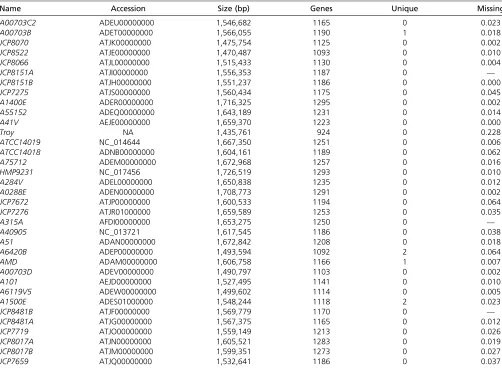
The number of genes and the number of unique genes present for each OTU in the gene database constructed with 2036 total number of genes are provided. A total of 558 genes were present in all OTUs. Note that the number of genes here refers to membership in gene families, not the total number of genes for each OTU. The missing data proportions are from method C, model 4 for theG. vaginalisanalysis.
Appendix B:MycobacteriumData
These genes may not be allocated to the same gene family as they might no longer cover 85% of the query. This is another mechanism of apparent gene gain, distinct from lateral gene transfer.
Appendix C: Gene Presence/Absence Patterns
The gene presence/absence patterns for theG. vaginalisandMycobacteriumspp. along with the respective trees are provided in a supplementary R package.
Appendix D: R Package
An R package namedindelmissis available from the Comprehensive R Archive Network (CRAN). The package canfit four models for estimating gene insertion/deletion rates. These four models estimate indel rates (where the insertion and deletion rates are forced to be equal), indel rates and proportions of missing data for taxa of interest, unique insertion and deletion rates, and unique insertion and deletion rates and proportions of missing data for taxa of interest, respectively (Table D1).
The package can also implement a correction for sampling bias, i.e, genes that were not observed for any of the OTUs. It is possible to simulate gene phyletic patterns for indel analysis as well as to provide custom trees and data. Furthermore, in lieu of weighting presence/absence contributions at the root of the tree by equilibrium frequencies (default behaviour), it is also possible to use equal weighting and user-specified probabilities and to estimate the probabilities at the root, using maximum likelihood. Moreover, clade or evolutionary-grade specific insertion and deletion rates can be estimated as well. The models have been optimized for speed with the recursive likelihood calculation written using theRcpppackage (Eddelbuettelet al.2011). Note that packagesmarkophylo(Dang and Golding 2016) andDiscML(Kim and Hao 2014) canfit models 1 and 3 (that do not account for missing data) as well.
Installation instructions
The following commands install indelmiss binaries from CRAN:
install.packages(“indelmiss”, dependencies = TRUE, repos =“
http://cran.r-project.org”)
Source package from CRAN
install.packages(“indelmiss”, dependencies = TRUE, repos =“
http://cran.r-project.org”, type =“source”)
If“-lgfortran”and/or“-lquadmath”errors are encountered on an OS X system, unpack fortran-4.8.2-darwin13.tar.bz2 from http://r.research.att.com/libs/into/usr/local. This issue has cropped up in the past with Rcpp/RcppArmadillo. Also, see the Rcpp FAQs vignette onhttps://cran.r-project.org/package=Rcpp/index.html.
Prior to installing an R package from source (download from CRAN) that requires compilation on Windows,Rtoolsneeds to be installed fromhttp://cran.r-project.org/bin/windows/Rtools/.Rtoolscontains MinGW compilers needed for build-ing packages requirbuild-ing compilation of Fortran, C, or C++ code. The PATH variable should be allowed to be modified during installation ofRtools.If this is not permitted, the PATH variable must be set to include“RTools/bin”and“Rtools/gcc-x.y.z/bin,” where“x.y.z”refers to the version number of gcc, following the installation ofRtools.Then,
install.packages(c(“Rcpp”,”ape”,”phangorn”, “numDeriv”, “testthat”), repos =
“http://cran.r-project.org”)
install.packages(“indelmiss_1.0.7.tar.gz”, repos = NULL, type =“source”)
Make sure the version number of indelmiss reflects the latest version on CRAN.
Appendix E: Simulation Set 3
We investigated cases where only the lineages with the highest apparent gene data loss on a given phylogeny are modeled with a proportion of missing data. Similar to simulation set 2, heterogeneous gene insertion and deletion rates among different lineages are simulated and analyzed in the presence of missing data. Five hundred random samples of 5000 gene presence/absence phyletic patterns were simulated for 10 taxa on the same tree (with the different-colored clades following different rates) as used in simulation set 2 (Figure 2). The patterns simulated using thephangornpackage followed the same parameters as those followed in simulation set 2. However, here, missing data were simulated at tipsf3;5;9g ðf1;6gÞby randomly and indepen-dently sampling from a uniform distribution between 0.2 (0) and 0.6 (0.15). Hence, for tips 1 and 6, a smaller proportion of missing data were randomly simulated than that for tips 3, 5, and 9. As in simulation set 2, no missing data were simulated at tips 2 and 8. Only tipsf3;5;9gwere allowed a missing data proportion. In effect, only those taxa are modeled with missing data proportions that have the highest apparent gene loss.
missing data proportion for tip 5 (Table E1; also note the ranges of the differences for the three tips). Missing data proportions for tips 3 and 9 are estimated very accurately but the missing data proportion for tip 5, although estimated with a reasonable magnitude, is somewhat biased. Figure E1 shows the differences between true and estimated rates, standardized by the true rates. Clearly, results based on the deletion rate for the gray clade (second row, middle column in Figure E1) are worse compared to the others. Deletion rates tend to be overestimated for the gray clade. While these results are intuitive, we urge caution in interpreting these results. Note that this is but one investigation of model misspecification. More work needs to be done to investigate this phenomenon in these phylogenetic comparative models.
Appendix F: PE/PPE Genes
When working withMycobacteriumspp. data, the PE/PPE genes are often left out of the analysis. Here, the gene family data set constructed inTwo examplesin the main text isfiltered to remove such gene families. This is done by removing any gene families with constituent genes that were associated with PE or PPE gene families as evidenced by their annotation in the downloaded genomes. A total of 7683 gene families were left in the database. The best-fitting model fromTwo exampleswas rerun here. The results are summarized in Table F1. Clearly, the parameter estimates here are close to the estimates inTwo examples.
Appendix G: Alternate Mycobacteriumspp. tree
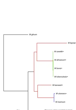
An alternate phylogenetic tree forMycobacteriumspp. was also constructed using MrBayes (Ronquist and Huelsenbeck 2003). This section illustrates the sensitivity of the studied models to the given phylogenetic trees. Multiple sequence alignments of nucleotide sequences of 50 genes found in each taxon were constructed using MAFFT (Katohet al.2002). These alignments were then concatenated and provided to MrBayes. A general time-reversible substitution model with gamma-distributed rate variation was run (1;000;000 generations with 25% burn-in) withM. gilvumspecified as the outgroup. A tree (without branch lengths) constructed using the PATRIC bacterial bioinformatics resource center (Wattamet al.2014) was provided to MrBayes as a starting tree for the algorithm. Ten random perturbations of the start tree were specified in MrBayes. The unrooted result from MrBayes had 100% support for every branch. Using Figtree (Rambaut 2014), this tree was rooted on the branch leading toM. gilvum. The pruned tree used inTwo examplesdiffers in the placement ofM. leprae(and branch lengths) from the tree constructed using MrBayes. Here, we analyze the gene family data set constructed inTwo examples, using the tree constructed using MrBayes in detail. Overall, the relative rates for the different-colored branches (see colored branches in Figure G1) in the best-fitting model are in agreement with the analysis inTwo examples.
Again, the best-fitting model fromTwo exampleswas rerun here. From this model,M. lepraeandM. ulceranshad estimated missing data proportions of^dM: leprae¼0:547ðSE¼0:011Þand^dM: ulcerans¼0:215ðSE¼0:009Þ(median missing data pro-portion is 0.026), respectively. The estimates of 0.547 and 0.215 correspond to 1687 and 758 genes, respectively. The branches in red in Figure G1 had an estimated rate of deletion m^1 ¼0:623ðSE¼0:034Þ and estimated rate of insertion ^
n1¼0:143ðSE¼0:010Þ:
The blue group in Figure G1, on the other hand, yielded m^2¼0:846ðSE¼0:544Þ and ^n2¼2:342ðSE¼0:190Þ: The branches in green (M. tuberculosis complex) had an estimated rate of deletionm^3¼1:715ðSE¼0:879Þand an estimated rate of insertion ^n3¼3:589ðSE¼0:283Þ: Finally, the black group yielded m^5 ¼0:749ðSE¼0:051Þ and ^
Figure G1 Phylogram for theMycobacteriumspp. data constructed us-ing MrBayes with the branch lengths measured in expected substitutions per site. The coloring of the branches corresponds to the grouping for model 4 from method B. The + signs indicate that a missing data pro-portion wasfitted for the associated taxa.Appendix Bgives references and strain information for these taxa.
Table B1 NCBI accession numbers with genome sizes for 10Mycobacteriumsequences
Name Accession Size (bp) Genes Unique Missing
M. gilvumPYR-GCK CP000656.1 5,547,747 5241 1239 —
M. lepraeTN NC_002677.1 3,268,203 1605 204 0.543
M. canettiiCIPT 140010059 NC_015848.1 4,482,059 3861 61 0.004
M. africanumGM041182 NC_015758.1 4,389,314 3830 28 0.023
M. bovisAF2122/97 NC_002945.3 4,345,492 3918 144 0.029
M. tuberculosisH37Rv NC_000962.3 4,411,532 3906 80 0.024
M. kansasiiATCC 12478 NC_022663.1 6,432,277 5712 1112 0.000
M. ulceransAgy99 NC_008611.1 5,631,606 4160 284 0.239
M. marinumM CP000854.1 6,636,827 5423 460 —
M. aviumMAP4 NC_021200.1 4,829,424 4326 504 —
The number of genes represents the number of coding sequences downloaded from NCBI. The number of genes unique to each OTU in the gene database is provided. There are 8034 total number of gene families in the database with a total of 959 genes present in all OTUs. The missing data proportions are from the best-fitting model 4 for the
Mycobacteriumspp. analysis.
Table A1 NCBI accession numbers with genome sizes for 35G. vaginalisstrains
Name Accession Size (bp) Genes Unique Missing
A00703C2 ADEU00000000 1,546,682 1165 0 0.023
A00703B ADET00000000 1,566,055 1190 1 0.018
JCP8070 ATJK00000000 1,475,754 1125 0 0.002
JCP8522 ATJE00000000 1,470,487 1093 0 0.010
JCP8066 ATJL00000000 1,515,433 1130 0 0.004
JCP8151A ATJI00000000 1,556,353 1187 0 —
JCP8151B ATJH00000000 1,551,237 1186 0 0.000
JCP7275 ATJS00000000 1,560,434 1175 0 0.045
A1400E ADER00000000 1,716,325 1295 0 0.002
A55152 ADEQ00000000 1,643,189 1231 0 0.014
A41V AEJE00000000 1,659,370 1223 0 0.000
Troy NA 1,435,761 924 0 0.228
ATCC14019 NC_014644 1,667,350 1251 0 0.006
ATCC14018 ADNB00000000 1,604,161 1189 0 0.062
A75712 ADEM00000000 1,672,968 1257 0 0.016
HMP9231 NC_017456 1,726,519 1293 0 0.010
A284V ADEL00000000 1,650,838 1235 0 0.012
A0288E ADEN00000000 1,708,773 1291 0 0.002
JCP7672 ATJP00000000 1,600,533 1194 0 0.064
JCP7276 ATJR01000000 1,659,589 1253 0 0.035
A315A AFDI00000000 1,653,275 1250 0 —
A40905 NC_013721 1,617,545 1186 0 0.038
A51 ADAN00000000 1,672,842 1208 0 0.018
A6420B ADEP00000000 1,493,594 1092 2 0.064
AMD ADAM00000000 1,606,758 1166 1 0.007
A00703D ADEV00000000 1,490,797 1103 0 0.002
A101 AEJD00000000 1,527,495 1141 0 0.010
A6119V5 ADEW00000000 1,499,602 1114 0 0.005
A1500E ADES01000000 1,548,244 1118 2 0.023
JCP8481B ATJF00000000 1,569,779 1170 0 —
JCP8481A ATJG00000000 1,567,375 1165 0 0.012
JCP7719 ATJO00000000 1,559,149 1213 0 0.026
JCP8017A ATJN00000000 1,605,521 1283 0 0.019
JCP8017B ATJM00000000 1,599,351 1273 0 0.027
Table D1 Gene insertion/deletion models available in indelmiss
Model m;n d
M1 E
M2 E ✓
M3 V
M4 V ✓
Here,m;n;andpare deletion rate(s), insertion rate(s), and proportion(s) of missing data for taxa of interest, respectively. Here, E implies that parametersmandnare equal, while V implies that they are free to vary.
Table E1 Averages and ranges for differences between simulated and estimated proportions of missing data for the corresponding taxa over 500 samples from simulation data set 3
Tip labels
Difference 3 5 9
di2^di 0.00 (20:02;0.03) 0.03 (20:01;0.08) 0.00 (20:02;0.02)
The tree in Figure 2 is used withm,n, anddisampled from a range of values (see text). While missing data are simulated onfive tips, only three of those are modeled with a proportion of missing data.
Table F1 Inferred insertion and deletion rates on a subset of the gene family data (without PE/PPE genes)
Group m^ ^n
Red 1:079 ðSE¼0:060Þ 0:411 ðSE¼0:026Þ
Green 2:034 ðSE¼0:968Þ 3:522 ðSE¼0:274Þ
Blue 1:173 ðSE¼0:880Þ 2:600 ðSE¼0:211Þ
Black 0:368 ðSE¼0:042Þ 0:251 ðSE¼0:017Þ