ABSTRACT
MEIJER, ALAN. Tillage Effects on Erosion, Soil Physical Properties, and Soil Moisture. (Under the direction of J.L. Heitman and J.G. White).
Tillage plays a key role in production agriculture soil management and can influence myriad
soil processes and properties, depending on its intensity. Tillage can chop and bury residue;
change soil physical structure; and alter how water moves on, into, and through the soil
matrix. If improperly implemented, it can lead to problems such as drought stress, poor root
penetration, and erosion. Consequently, it is important to understand how soils are affected
by long-term tillage practices. Our research examined tillage practices at a long-term (28
year) research site in the North Carolina piedmont. Our primary objectives were to determine
the effects of tillage on: 1) soil erosion using ground-based lidar; 2) soil physical properties
such as bulk density, particle size distribution, water retention, plant-available water, carbon,
and carbon stratification ratio in three row positions (in-row, trafficked interrow, and
untrafficked interrow) and to depths of 105 cm; and 3) soil profile moisture conditions to
estimate water-use efficiency and depletion and recharge during and following dry periods.
The tillage methods were no-till (NT), in-row subsoiling (IRS), chisel plow in spring (CHsp)
or fall (CHfa), disk (D), chisel plow in spring or fall followed by disk (CHspD, CHfaD) and
moldboard plow in spring or fall followed by disk (MPspD, MPfaD). Soil type at the site was
a Casville sandy loam (fine, mixed, semiactive, mesic Typic Kanhapludult). Lidar elevation
data showed that the natural elevation gradient (i.e., trend) at the site was best removed using
a second order polynomial; the de-trended data were used for analysis of erosion losses. The
Mt ha-1. In general, estimated soil loss was greatest in tillage treatments of higher tillage intensity. Bulk density was greatest in the trafficked row position of all treatments, an effect
detected only at a depth of 10 cm. Particle size distribution was not affected by tillage and
changed only with depth. Few differences were detected for water retention and
plant-available water. Carbon content was greatest at 2.5 cm and decreased substantially with
depth, especially in low tillage intensity treatments such as NT and IRS. The carbon
stratification ratio that compared shallow (2.5 cm) vs. deeper depths (10 cm) was greatest in
NT, CHsp, and D. Treatments with the greatest carbon stratification ratios tended to be the
same treatments that produced the greatest yields over the life of the study. Water-use
efficiency was highest in NT and IRS, and lowest in CHsp and MPspD in all five years that
soil moisture data were collected. During periods of near-zero rainfall, more water was
removed from the soil profile in low-intensity tillage treatments than others, and
subsequently these treatments gained more water after rainfall, indicating the influence of
tillage on a soil’s ability to provide water during dry periods. Overall, results show that
conditions conducive to crop growth, yield, and soil conservation coincided with long-term
© Copyright 2013 by Alan D. Meijer
Long-term Tillage Effects on Soil Erosion, Physical Properties, and Soil Moisture
by Alan D. Meijer
A dissertation submitted to the Graduate Faculty of North Carolina State University
in partial fulfillment of the requirements for the degree of
Doctor of Philosophy
Soil Science
Raleigh, North Carolina
2013
APPROVED BY:
_______________________________ ______________________________ Dr. Josh Heitman Dr. Jeff White
Committee Co-chair Committee Co-chair
DEDICATION
This dissertation is dedicated to my wife Charlene, our children Catherine, Laurel, Seth, and
Lily; my parents Max and Liz Meijer; my in-laws Holly and the late Case Van Staalduinen;
BIOGRAPHY
Alan was born in Hamilton, Ontario, Canada. He graduated from Smithville District
Christian High School in 1989 and earned a B.Sc. in Biology at Redeemer College in
Ancaster, Ontario in 1994. From 1996 - 2006, Alan worked as a technician for Dr. Ron
Heiniger of NC State University’s Crop Science Department, earning both a Graduate
Certificate in Geographic Information Systems (2002) and a M.Sc. in Crop Science (2004)
during that time. The title of Alan’s thesis was “Characterizing a Crop Water Stress Index for
Predicting Yield in Corn”. Throughout those years, a strong interest in, GIS, precision
farming, and the spatial dependence of natural phenomena grew. In 2006, Alan accepted a
position as an Extension Associate for Tillage and Soil Management in the Soil Science
Department at NC State University, and started working on his Ph.D. in Soil Science in 2008.
Alan continues to live in eastern North Carolina with his wife, Charlene, and their four
ACKNOWLEDGEMENTS
I am extremely grateful for the enduring patience of my advisor, Dr. Josh Heitman, and for
the wisdom he imparted to me over the duration of this work. The time and thought he has
put into my efforts have been invaluable to me. I am also indebted to my co-advisor, Dr. Jeff
White, for taking me on in this project, and for the advice and knowledge he has shared with
me regarding a host of subjects. I would like to thank Dr. Michael Wagger and Dr. Ron
Heiniger, for the role they played throughout as part of my graduate advisory committee.
I sincerely appreciate the opportunity provided, and support given, by Michael Wagger,
Department Head; and Deanna Osmond, Department Extension Leader, as I pursued this
degree. I always hoped that my pursuit of this degree would benefit not only myself, but the
department and the citizens of North Carolina as well.
Robert Walters has overseen the Reidsville tillage trials since 1994 and they obviously mean
a lot to him. Without his continued dedication to the work being done there, this work, and
much of the previous would not have been possible.
Adam Howard is a technical genius and all-around hard worker. His no-bull attitude and
efficient mindset was invaluable to me throughout this work.
I am extremely grateful to Jennifer Amick Etheridge as she worked diligently at running
particle size analysis and water retention on thousands of samples, not to mention grinding
Rob Austin is a GIS wizard. His work with the ground-based lidar was crucial in
accomplishing that part of this dissertation. Thanks, Rob.
There are numerous folks from the Soil Science department that have helped tremendously
during the core sampling process. Those I am grateful to in this regard include: Scott King,
Weinan Pan, Matt Taggart, Mark Connolly, Chris D’Aiuto, Colby Moorberg, and Stephen
Holland.
Joe French, Aileen Dyson, and the rest of the staff at the Upper Piedmont Research Station
have cheerfully helped in the various aspects of accomplishing this research. Joe and his
crew have managed much of the tillage and spraying of plots, while Aileen has provided
years of rainfall data from diligent daily task of recording the day’s rainfall totals.
Joy Smith of NCSU’s Statistics Department was instrumental in helping me sort out a lot of
SAS code. Her extensive knowledge of statistics and SAS programming is admirable, and I
always felt better about my work after meeting with her. Thanks, Joy. It was a pleasure to get
to know Dr. Dickey a little better after having him as an instructor for ST512 back in 2000.
When I asked him if I needed to take the analysis a step further, he replied: “We can make
this as complicated as you’d like, but I believe this here will work fine”. Thanks, Dr. Dickey.
Carl Crozier and Dominic Reisig, my colleagues at the Vernon James Center, have been a
great deal of help to me. Carl has offered advice on a variety of topics, and Dominic has been
I sincerely thank Barry Tarleton for offering me a place to stay many times when I was in
Raleigh multiple days in a row. You would give the shirt off your back, and I appreciate it. I
just can’t believe your neighbors!
Wes Tuttle (NRCS) was great to work with. While our research involving ground-penetrating
radar did not make it into this body of work, I’ve enjoyed our work together. Extremely
knowledgeable about soils, new remote sensing technologies, as well as baseball and all
things bluegrass, it’s a pleasure to know him. I hope to catch up with him at Merlefest
someday and pick a few tunes with you and your accomplished bluegrass buddies.
I offer thanks to the North Carolina Soybean Producers Associate and the Corn Growers
Association of North Carolina for their monetary support, making this project possible.
I would first like to thank my wife, Charlene, for her enduring love and support in the pursuit
of this goal. It would simply have been impossible for me to finish this process without her
unending encouragement and hard work. Raising four young children, with me being gone so
much due to classes and work was a significant burden that she never once complained
about. The unconditional love of my children Catherine, Laurel, Seth and Lily has been a
source of joy for me. I appreciate the support given by my in-laws, Holly and the late Case
Van Staalduinen, and my parents, Max and Liz Meijer, for their continued love and support.
Firstly, and yet last on this list, I’m thankful to the Lord my God, for His love, strength,
TABLE OF CONTENTS
LIST OF TABLES ... xi
LIST OF FIGURES ... xiii
1. Introduction ...1
1.1 Research Objectives and dissertation organization ...3
1.2 References ...6
2. Measuring Erosion in Long-Term Tillage Plots Using Ground-Based Lidar ...9
2.1 Introduction ...10
2.2 Materials and Methods ...16
2.2.1 Location and Soils...16
2.2.2 Experimental Design & Treatments...16
2.2.3 Lidar Scanning ...18
2.2.4 Trend Removal ...19
2.2.5 Soil loss calculation ...21
2.2.6 Analysis...21
2.3 Results and Discussion ...22
2.3.1 Lidar Scanning ...22
2.3.3 Analysis of Variance ...24
2.3.4 Treatment Effects on Soil Elevation ...25
2.3.5 Treatment Effects on Soil Loss ...27
2.4 Summary and Conclusions ...28
2.5 References ...31
3. Tillage, depth, and traffic effects on soil physical properties and yield in a long-term tillage study in the North Carolina Piedmont. ...47
3.1. Introduction ...48
3.2. Materials and Methods ...53
3.2.1. Location, Soils, and Cropping System ...53
3.2.2. Experimental Design & Treatments ...53
3.2.3. Cultural practices ...54
3.2.4. Soil physical and properties ...54
3.2.5. Carbon and Carbon Stratification ...56
3.2.6. Statistical Analyses ...56
3.3. Results and Discussion ...57
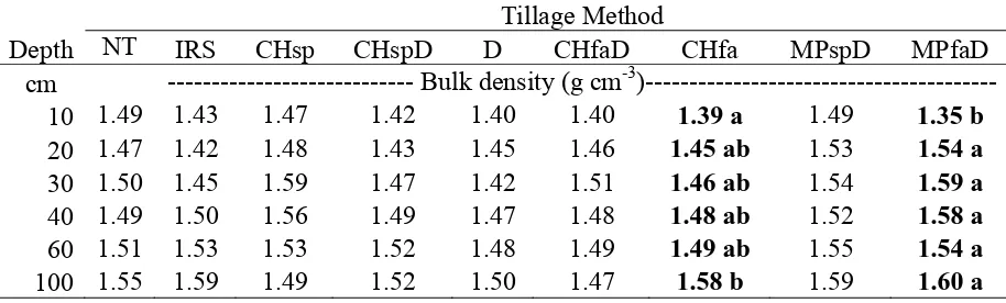
3.3.1. Bulk density ...57
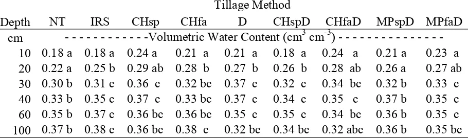
3.3.2 Volumetric Water Content...60
3.3.4. Water Retention ...62
3.3.5. Plant Available Water ...63
3.3.6. Carbon and Carbon Stratification Ratio ...64
3.3.7 Crop Yield ...65
3.4. Summary and Conclusions ...66
3.5 References ...69
4. Effects of nine long-term tillage systems on soil moisture in the North Carolina Piedmont ...91
4.1 Introduction ...92
4.2. Materials and Methods ...95
4.2.1. Location, Soils, and Cropping System ...95
4.2.2. Experimental Design & Treatments ...96
4.2.3. Cultural practices ...96
4.2.4 Soil Profile Moisture Monitoring ...97
4.2.5 Precipitation and Evapotranspiration ...98
4.2.6 Critical Growth Periods ...98
4.2.7 Water Use Efficiency ...99
4.2.8 Depletion and Recharge Events ...99
4.3. Results ...100
4.3.1 Precipitation ...100
4.3.2 Crop Yield ...101
4.3.3 Soil Profile Moisture ...102
4.3.4 Critical Growth Period Soil Moisture ...103
4.3.5 Water Use Efficiency ...104
4.3.6 Soil Moisture Depletion and Recharge ...104
4.4. Summary and Conclusions ...106
4.5 References ...109
5. Summary and Conclusions ...124
5.1 Suggestions for future work ...127
LIST OF TABLES
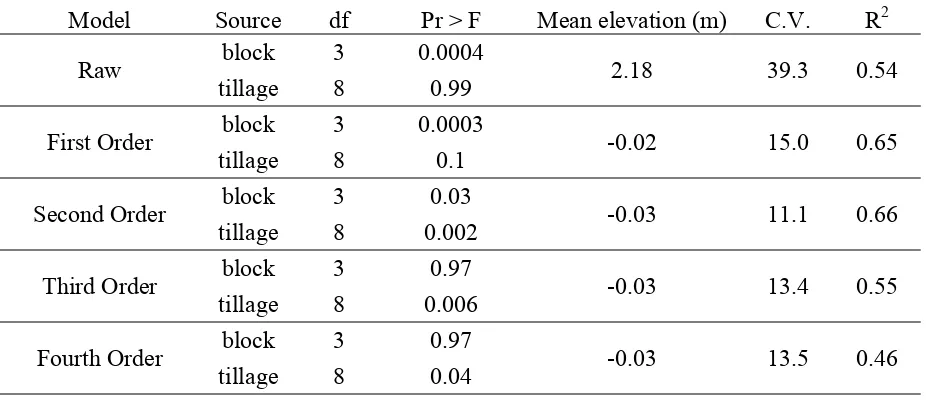
Table 2.1 Results of ANOVA for the effect of block and tillage treatment on elevation for raw and detrended data. Model column indicates which model was used to detrend the data. ... 37
Table 2.2 Mean treatment values for bulk density, weighted by row position. P-value: 0.007.Least square means adjustment method for multiple comparisons: Tukey. NT, no-till; IRS, in-row subsoiling; CHfa, fall chisel; CHsp, spring chisel; D, disk; CHfaD, fall chisel plus disk; CHspD, spring chisel plus disk; MPfaD, fall moldboard plow plus disk; MPspD, spring moldboard plow plus disk. ... 38
Table 2.3 Results of ANOVA for effect of tillage on soil loss or gain for the second-order dataset assuming zero soil loss in the no-till system. Treatment means are shown in Fig. 2.7. ... 39
Table 3.1 Analysis of variance p values for the effects of tillage, depth, and position on bulk density (ρβ) and volumetric soil water content at sampling (θv), and the effects of tillage and
depth on all other parameters (where positions were not sampled). T, tillage; P, position; D, depth; θ10, θ30, θ100, θ500, θ1500, volumetric water retention at matric pressures of 10, 30, 100, 500, and 1500 kPa, respectively; PAW10, PAW30, plant-available water using 10-kPa and 30-kPa field capacity, respectively; C, carbon; CSR1, stratification ratio of carbon at 0-5 cm to that of 5-15 cm; CSR2, carbon stratification ratio of carbon at 0-5 cm to that of 15-25 cm. .. 75
Table 3.2 Simple effects of depth on bulk density by tillage method, averaged over row position. Within bolded columns, means followed by different letters indicate Tukey-adjusted means separation (α = 0.05). There were no significant differences among tillage treatments by depth. NT, no-till; IRS, in-row subsoiling, D, spring disk; CHfa, fall chisel plow; CHsp, spring chisel plow; CHfaD, fall chisel plow plus spring disk; CHspD, spring chisel plow plus spring disk; MPfaD, fall moldboard plow plus spring disk; MPspD, spring moldboard plow plus spring disk. ... 76
Table 3.3 Simple effects of depth on volumetric water content by tillage method. Within columns, means followed by different letters indicate Tukey-adjusted means separation (α = 0.05). NT, no-till; IRS, in-row subsoiling, D, spring disk; CHfa, fall chisel plow; CHsp, spring chisel plow; CHfaD, fall chisel plow plus spring disk; CHspD, spring chisel plow plus spring disk; MPfaD, fall moldboard plow plus spring disk; MPspD, spring moldboard plow plus spring disk. Simple effects of tillage method within depth were not detected. ... 77
means separation (α = 0.05) for the simple effects of row position by depth. R, in-row; T, trafficked interrow; U, untrafficked interrow. ... 78
Table 3.5 Main effect of tillage method on water retention for matric potentials tested, averaged over depth. Tukey-adjusted means separation (α = 0.05). NT, no-till; IRS, in-row subsoiling, D, spring disk; CHfa, fall chisel plow; CHsp, spring chisel plow; CHfaD, fall chisel plow plus spring disk; CHspD, spring chisel plow plus spring disk; MPfaD, fall moldboard plow plus spring disk; MPspD, spring moldboard plow plus spring disk. ... 79
Table 3.6 Main effect of depth on water retention for matric potentials tested, averaged over tillage treatments. Within columns, means followed by different letters indicate Tukey-adjusted means separation (α = 0.05)... 80
Table 3.7 Main effect of tillage method on plant-available water using field capacity estimated at both 10 and 30 kPa. Letters within columns denote significant differences (α = 0.05). NT, no-till; IRS, in-row subsoiling, D, spring disk; CHfa, fall chisel plow; CHsp, spring chisel plow; CHfaD, fall chisel plow plus spring disk; CHspD, spring chisel plow plus spring disk; MPfaD, fall moldboard plow plus spring disk; MPspD, spring moldboard plow plus spring disk. ... 81
Table 3.8 Main effect of depth on plant-available water calculated using field capacity at both 10- and 30-kPa (PAW10 and PAW30). Letters within columns denote significant differences (α = 0.05). ... 82
Table 4.1 Planting and harvest dates for crops from 2008-2012. ... 113
Table 4.2 Details regarding depletion periods (DP) and recharge (RC) events targeted for study. Recharge dates were chosen based on a minimum of 10 consecutive days with precipitation <0.5 cm, followed by precipitation > 1.0 cm. 2008 and 2012 had no periods meeting these criteria. ... 114
Table 4.3 Precipitation for the Upper Piedmont Research Station in Reidsville, NC, from 2008 to 2012. Shaded months indicate the main months in the crop growing season for a given year; see Table 4.1 for exact dates. S, soybean; C, corn; CV, coefficient of variation. ... 115
Table 4.4 P-values for the effects of tillage, depth, and sampling date on soil moisture and their interactions for all sampling dates from 2008 to 2012, by year. S, soybean; C, corn. . 116
Table 4.5 Effect of tillage on net change in mean soil water content through 40 cm depth for each of four depletion periods (DP) and their associated periods of recharge (RC). ... 117
LIST OF FIGURES
Fig. 2.1 Aerial image, trial boundary, and airborne lidar-derived 0.6-m elevation contours for the Nine Tillage Study. Slope decreases from the east to the west. This image was made approximately 3 weeks after lidar scanning. Location of blocks and many individual tillage plots are visible. Image date: 7 July 2010. Source: Google Inc. Elevation contours source: NC Floodplain Mapping Program. Date: 2007. ... 40
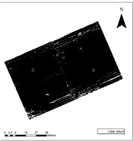
Fig. 2.2 Location of lidar returns from four scans in the Nine-Tillage Study. Each black dot represents one return (data point) of a laser pulse to the scanner head. Four circular areas indicate location of scanner in the alleys (between blocks) of the experiment. Linear WSW to ENE features with no returns (white) indicates areas not visible to the scanner behind a ridge of soil. ... 41
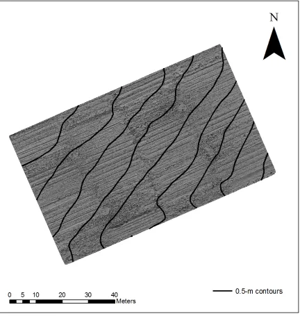
Fig. 2.3 A hillshaded Triangulated Irregular Network (TIN) created from raw elevation values (trend intact). Hillslope indicated by 0.5-m contours. ... 42
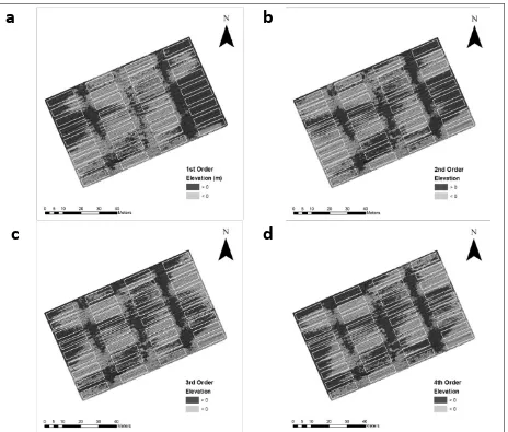
Fig. 2.4 Oblique representation of trend surfaces modeled using (a) first- , (b) second-, (c) third-, and (d) fourth-order polynomials. Vertical elevations were exaggerated 20x to better show effect of higher-order models on trend-surface complexity. Elevation contours represent 0.25 m of elevation change. Grayscale gradient illustrates high (dark gray) to low (light gray) elevations. Surfaces have been tilted to effectively show shape of surface. ... 43
Fig. 2.5 Hillshaded TINs created from data detrended using a (a) first-, (b) second-, (c) third-, and (d) fourth-order polynomial. Data were classified to illustrate areas above (> 0) and below (< 0) the trend. White polygons indicate location of AOIs. ... 44
Fig. 2.6 Mean elevations of tillage treatments relative to the trend for data detrended with first- through fourth-order polynomials. Treatment columns within one panel differ significantly when labeled with different letters (LSD, p ≤ 0.05). Error bars are standard errors. NT, no-till; IRS, in-row subsoiling; CHfa, fall chisel; CHsp, spring chisel; D, disk; CHfaD, fall chisel plus disk; CHspD, spring chisel plus disk; MPfaD, fall moldboard plow plus disk; MPspD, spring moldboard plow plus disk. ... 45
Fig. 3.1 Simple effects of depth on bulk density by row position. Within row positions, means followed by different letters indicate Tukey-adjusted means separation (α = 0.05). R, in-row; T, trafficked interrow; U, untrafficked interrow. ... 83
Fig. 3.2 Simple effects of row position on bulk density by depth. Within depths, means followed by different letters indicate Tukey-adjusted means separation (α = 0.05). ... 84
Fig. 3.3 Effects of depth on percent sand, silt, and clay. Within column segments, different letters indicate Tukey-adjusted means separation (α = 0.05)... 85
Fig. 3.4 Water release curves by tillage method. Significant differences between treatments at 33 and 100 kPa are denoted by larger symbols. ... 86
Fig. 3.5 Simple effects of depth on percent C by tillage method. Within tillage treatments, means followed by different letters indicate Tukey-adjusted means separation (α = 0.05). NT, no-till; IRS, in-row subsoiling; D, disk; CHfa fall chisel plow; CHfaD, fall chisel plow plus disk; MPfaD, fall moldboard plow plus disk. ... 87
Fig. 3.6 Simple effects of tillage method on percent C by depth. Within depths, means followed by different letters indicate Tukey-adjusted means separation (α = 0.05). NT, no-till; IRS, in-row subsoiling; D, disk; CHfa fall chisel plow; CHfaD, fall chisel plow plus disk; MPfaD, fall moldboard plow plus disk. ... 88
Fig. 3.7 Main effect of tillage on the ratio of C at 0 to5 cm to 5 to15 cm (CSR1). Means followed by different letters indicate Tukey-adjusted means separation (α = 0.05). NT, no-till; IRS, in-row subsoiling, D, spring disk; CHfa, fall chisel plow; CHsp, spring chisel plow; CHfaD, fall chisel plow plus spring disk; CHspD, spring chisel plow plus spring disk; MPfaD, fall moldboard plow plus spring disk; MPspD, spring moldboard plow plus spring disk. ... 89
Fig. 3.8 Tillage treatment effects on long-term (1988-2011) corn and soybean yield means. Means within crop followed by different letters indicate Tukey-adjusted means separation (α
= 0.05). NT, no-till; IRS, in-row subsoiling, D, spring disk; CHfa, fall chisel plow; CHsp, spring chisel plow; CHfaD, fall chisel plow plus spring disk; CHspD, spring chisel plow plus spring disk; MPfaD, fall moldboard plow plus spring disk; MPspD, spring moldboard plow plus spring disk. ... 90
Fig. 4.2 Crop yields from 2008 - 2012 at the Nine Tillage Study. Columns within years followed by different letters are significantly different at α = 0.05. NT, no-till; IRS, in-row subsoiling; CHsp, spring chisel; D, disk; CHspD, spring chisel plus disk; MPspD, spring moldboard plow plus disk. ... 119
Fig. 4.3 Main effects of tillage on soil water content during the critical growth period 60 to 90 days after corn planting averaged over 2009 and 2011. Columns marked by different letters are significantly different at α = 0.05. NT, no-till; IRS, in-row subsoiling; CHsp, spring chisel; D, disk; CHspD, spring chisel plus disk; MPspD, spring moldboard plow plus disk. ... 120
Fig. 4.4 Effects of tillage on water use efficiency from 2008 – 2012. Columns within years followed by different letters are significantly different at α = 0.05. NT, no-till; IRS, in-row subsoiling; CHsp, spring chisel; D, disk; CHspD, spring chisel plus disk; MPspD, spring moldboard plow plus disk; soy, soybean. ... 121
Fig. 4.5 Precipitation and mean soil profile water content of three tillage treatments during the 2010 dry-down and recharge event (DP2 and RC2), a year when soybeans were grown. NT, no-till; IRS, in-row subsoiling; MPspD, spring moldboard plow plus disk. Treatments shown here were selected to indicate that range of net change in soil moisture content in the data. ... 122
1. Introduction
Tillage has been a part of growing crops since the advent of agriculture and has played a role
in allowing more land to be made arable and for fewer people to produce food for an ever
increasing population. However, altering a soil’s physical state from native and untouched to
one disrupted by tillage can be dramatic and has caused a number of severe problems
throughout history, even to the extent of degrading the soil to a greater degree in less time in
this era than at any point throughout history (Faulkner, 1943).
The various physical, chemical, and biological processes that occur within the soil profile are
partially governed by soil physical properties, all of which can be altered by the physical
disruption of soil that occurs with tillage and the trafficking of the soil surface with farm
equipment. By mixing and breaking up the natural soil structure and aggregation of soil
particles, properties such as bulk density (Hill and Cruse, 1985), soil strength (Ehlers et al.,
1983; Lindstrom et al., 1984; Tollner et al., 1984), and porosity (Voorhees and Lindstrom,
1984) are dramatically altered. These changes can adversely affect root penetration (Ehlers et
al., 1983), infiltration (Lindstrom and Onstad, 1984; Freese et al., 1993), runoff (Afunyi,
1997), and soil water retention (Bescansa et al., 2006), which can all affect crop growth.
Impacts of tillage on soil water relations are of particular importance. Before water can move
through a soil, it must first infiltrate. Tillage can foster conditions of compacted or crusted
soil surfaces which limit infiltration (Freese et al., 1993; Pikul and Zuzel, 1994). In tilled
particles are dislodged by the force of the moving water (Lal, 1994). Additionally, soils can
suffer from wind erosion.
In the mid-1980s, there was a shift towards conservation tillage methods that involved little
soil mixing and left much of the plant residue on the surface. These tillage methods were
known collectively as conservation tillage practices. With the soil surface covered year-round
with living plants or residue, infiltration may be improved along with a corresponding
reduction in erosion (Brady and Weil, 2002). With less residue incorporation into soil,
organic matter breaks down at a reduced rate, allowing for its buildup on or just below the
soil surface. Soil organic matter is known to benefit soil physical, chemical, and biological
properties by increasing aggregation; infiltration; decomposition and nutrient cycling; and
biological activity (Franzluebbers, 2010). Conservation tillage use has been increasing in the
United States, from approximately 71 million acres in 1989 to almost 114 million acres in
2008 (Conservation Technology Improvement Center, 2008).
In some areas, such as the Great Plains region of the United States where irrigation water is
pumped from the shrinking Ogallala aquifer, water resources are more limited now than what
they once were. With the natural limitation of rainfall, and a natural or potentially legislated
limitation on irrigation, the need for efficient soil water storage and use efficiency is critical.
The Nine Tillage Study was implemented in 1984 in an effort to determine tillage practices
that improve infiltration, reduce erosion, and improve crop yields for growers in the
of tillage intensity and soil disturbance were tested. These ranged from moldboard plowing
through no-till.
Numerous experiments have been conducted at the Nine Tillage Study, with varied
objectives and methods. Early work focused on the effects of two years of tillage on soil
physical properties such as bulk density and cone index (Cassel et al., 1995). In 1998,
research shifted to processes such as infiltration and runoff (Freese et al., 1993; Myers and
Wagger, 1996). Unpublished work related to macroaggregate stability, volumetric porosity,
and plant-available water has been carried out and briefly summarized in proceedings papers
(White et al., 2009).
Technologies that utilize non-invasive techniques to estimate or measure some parameter of
the soil continue to be developed and have provided new methods for understanding the
current status of soils. Lidar is one such technology; it has been used to characterize
topography, with data usually captured from an airplane. A recent development of the
technology has allowed this data to be collected in an extremely dense manner in a
ground-based system. This method of collecting elevation data can be used to characterize long-term
effects of soil management techniques on a soil’s surface.
1.1 Research Objectives and dissertation organization
We undertook research to study the effects that 28 years of various tillage methods have had
on: soil erosion and physical condition; moisture available for crops; and long- and
loss using ground-based lidar scanning; 2) determine the effects of tillage, traffic (row
position), and depth on soil physical properties; and 3) examine the effects of tillage on soil
moisture parameters at multiple depths.
To address Objective 1, a ground-based laser scanner was used to generate a cloud of points
representing the soil surface (Kessler et al., 2012). Polynomial linear regression was used to
apply a 2nd order model to remove the effects of hillslope, leaving elevation data representing the relative elevations of the individual plots. From these, soil loss and accumulation were
estimated relative to the no-till treatment, which was considered the most stable soil surface
over the history of the experiment (Chapter 2).
To address Objective 2, tillage treatment effects on soil physical properties were determined
from non-intact soil cores extracted from the in-row, trafficked, and untrafficked interrow
positions at depths centered at 2.5, 10, 20, 30, 50, 60, and 100 cm. We tested for the effects
of tillage, depth, and row position on soil bulk density and volumetric water content. We also
tested the effects of tillage and depth on: percent sand, silt, and clay; water-retention at 10,
30, 100, 500, and 1500 kPa; plant-available water from 5- to 45-cm depth; total carbon; and
carbon stratification ratio (Chapter 3).
To address Objective 3, soil moisture data were recorded periodically since 2008. Using
access tubes installed in six of the nine tillage treatments, volumetric soil water content was
measured with a capacitance probe at depths of 10, 20, 30, 40, 60, and 100 cm. The resulting
periods, as well as the subsequent increase in water content following rainfall (Chapter 4).
Chapter 5 summarizes our work and conclusions.
1.2 References
Afunyi, M.M., Wagger, M.G., Leidy, R.B., 1997. Runoff of two sulfonylurea herbicides in
relation to tillage system and rainfall intensity. J. Environ. Qual. 26, 1318-1326.
Bescansa, P., Imaz, M.J., Virto, I., Enrique, A., Hoogmoed, W.B., 2006. Soil water retention
as affected by tillage and residue management in semiarid Spain. Soil Till. Res. 87,
69-75.
Brady, N.C., Weil, R.R., 2002. The nature and property of soils. 13th ed. Prentice-Hall. New York.
Cassel, D.K., Raczkowski, C.W., Denton, H.P., 1995. Tillage effects on corn production and
soil physical conditions. Soil Sci. Soc. Am. J. 59, 1436-1443.
Conservation Technology Information Center, 2008. National survey of conservation tillage
practices. West Lafayette, IN. http://www.ctic.org/CRM/crm_search/ (confirmed 17 Jul
2013)
Ehlers, W., Koke, W., Hesse, F., Bohm, W., 1983. Penetration resistance and root growth of
oats in tilled and untilled loess soil. Soil Till. Res. 3, 261-275.
Franzluebbers, A.J., 2010. Depth distribution of soil organic carbon as a signature of soil
Freese, R.C., Cassel, D.K., Denton, H.P., 1993. Infiltration in a piedmont soil under three
tillage systems. J. Soil Water Conserv. 48(3), 214-218.
Faulkner, E., 1943. Plowman’s Folly. Grosset and Dunlap, New York.
Hill, R.L., Cruse, R.M., 1985. Tillage effects on bulk density and soil strength. Soil Sci. Soc.
Am. J. 49, 1270-1273.
Kessler, A.C., Gupta, S.C., Dolliver, H.A.S., Thoma, D.P., 2012. Lidar quantification of bank
erosion in Blue Earth County, Minnesota. J. Environ. Qual. 41, 197-207.
Lindstrom, M.J., Onstad, C.A., 1984. Influence of tillage systems on soil physical properties
and infiltration after planting. J. Soil Water Conserv. 39, 149-152.
Lindstrom, M.J., Voorhees, W.B., Onstad, C.A., 1984. Tillage system and residue cover
effects on infiltration in northwestern corn belt soils. J. Soil Water Conserv. 39, 64-68.
Myers, J.L., Wagger, M.G., 1996. Runoff and sediment loss from three tillage systems under
simulated rainfall. Soil Till. Res. 39, 115-129.
Pikul Jr., J.L., Zuzel, J.F., 1994. Soil crusting and water infiltration affected by long-term
tillage and residue management. Soil Till. Res. 66, 95-105.
Stocking, M.A., 1994. Assessing soil vegetative cover and management effects, in: Lal, R.
Tollner, E.W., Hargove, W.L., Langdale, G.W., 1984. Influence of conventional and no-till
practices on soil physical properties in the southern Piedmont. J. Soil Water Conserv. 39,
73 -76.
Voorhees, W.B., Lindstrom, M.J., 1984. Long-term effects of tillage method on soil tilth
independent of wheel traffic compaction. Soil. Sci. Soc. Am. J. 48, 152-156.
White, J.G., Walters, R.D., Heitman, J.L., Howard, A.M., Wagger, M.G., 2009. Long-term
conservation tillage effects on soil physical properties and productivity of southeastern
U.S. Piedmont soils. In Annual meetings abstracts [CD-ROM]. ASA, CSSA, andSSSA,
2. Measuring Erosion in Long-Term Tillage Plots Using Ground-Based Lidar
A manuscript published in Soil and Tillage Research (Vol. 126 (2013) 1-10).
A.D. Meijera, J.L. Heitmanb, J.G. Whiteb, R.E Austinb (1) NC State University, Plymouth, NC 27962
(2) NC State University, Raleigh, NC, 27695, United States
Abstract
Erosion remains a serious problem for agricultural soils throughout the world. Tillage
significantly affects a soil’s susceptibility to erosion. Erosion research is usually conducted in
situ by capturing eroded sediment in brief, natural or artificial rainfall events. Methods for
measuring long-term erosion are needed to better understand long-term effects of soil
management. Landscape change resulting from erosion may be accurately characterized
using ground-based lidar. Ground-based lidar data were collected in 2010 at a long-term
(28-yr) trial of nine tillage treatments in the North Carolina Piedmont. Tillage effects on
plot-surface elevations were examined after removing large-scale variation in elevation (slope) by
detrending with first- through fourth-order polynomials. Residuals represented the elevation
difference from the trend for each location. Mean plot elevations were calculated for datasets
from each detrending model and used to assess erosion. In the subsequent elevation analysis,
data derived from the second-order polynomial had the highest R2, attributing 66% of the variation in elevation to block and treatment. Treatment elevations relative to no-till (NT)
ranged from +3.20 cm in the fall chisel (CHfa) plots to -13.28 cm in the fall moldboard plow
intensely-tilled treatments had the lowest elevations and the least-tilled treatments had the
highest. NT was used as the reference elevation for no change, and soil loss was calculated
using these data along with field-collected estimates of bulk density. The relative elevation
differences corresponded to a maximum treatment mean soil loss of 1891 Mg ha-1, which corresponds to an average annual soil loss of 67.5 Mg ha-1 yr-1. Soil loss estimates were similar to others estimated from soil profile truncation. This research indicates that
ground-based lidar data can be used to estimate soil elevation changes and thus soil loss due to
tillage-induced erosion.
2.1 Introduction
Erosion is a serious and well-documented problem with 1.73 Gt of soil lost from agricultural
fields in the U.S.A. annually (Hassel, 2005). Erosion leads to the sedimentation of
waterways, air quality degradation, the transport of nutrients and pesticides offsite, and the
loss of topsoil, organic matter, nutrients, and soil productivity in agricultural areas. Erosion
rates vary with rainfall duration and intensity; tillage method, timing, and frequency; soil
type, and slope (Chouhadry et al., 1997; Meyer and Harmon, 1989; Valmis et al., 2004).
Soils exposed to wind, rainfall, and runoff are most susceptible to erosion. Minimizing runoff
and optimizing infiltration by maintaining plant residue cover and soil aggregation are
critical to reducing erosion (Raczkowski et al., 2009, Raczkowski et al., 2002).
Tillage method largely determines a soil’s susceptibility to erosion. The physical action of
quantity of residue left intact. In a simulated rainfall study on continuous corn (Zea mays, L.)
on moderately (5%) sloping land in Nebraska, Dickey et al. (1984) measured residue cover
and corresponding soil loss in various tillage operations. After applying water at a rate of 64
mm h-1 until runoff rates reached equilibrium (usually around 45 minutes, equaling 51 mm of simulated precipitation), they found that for moldboard plow (MP), chisel plow (CH), disk
(D), and no-till (NT), where residue cover was 4, 17, 16 and 51%, soil loss was 46, 21, 19,
and 6 Mg ha-1 h-1, respectively. Tillage also moves soil laterally in the same direction the implement is being pulled, a process called tillage erosion. Studies show that soil is most
susceptible to this type of displacement in convex landscape positions (Govers et al., 1994;
Lindstrom et al., 1992; Lobb et al., 1995). Net soil movement occurs from convex to concave
landscape positions even if tillage is performed in both directions. Over time, erosion results
in surface elevation change: negative in areas of erosion and positive in areas of deposition.
Tillage can also affect the bulk density of the soil (Fraser et al. 2010). Soils with a lower bulk
density occupy greater volumes, often resulting in an increased surface elevation as
compared to that of a similar soil with higher bulk density. This effect may be transient as the
soil compacts over time following tillage and may also confound short-term vs. long-term
effects of erosion on surface elevation.
The effects of tillage on soil physical properties have been studied since 1984 at the Nine
Tillage Study (NTS), a long-term tillage study in Reidsville, NC. At the initiation of the
study, the use of moldboard plow and disk was common in Piedmont-region agriculture
water storage, reduce soil erosion, and increase crop yield for regional growers (Cassel et al.,
1995). The sandy clay loam at this site was prone to drought-stress (Denton and Wagger,
1992), highly erodible, subject to crusting, and typical of Piedmont soils used extensively for
agriculture (Cassel et al., 1995), making the site suitable for testing various tillage systems.
Nine tillage treatments were used in the study, representing a range of tillage intensity
including; NT, CH, and MP. Residue cover in these systems ranged from 0% in moldboard
plow plots to 98% in NT plots (Freese et al., 1993).
At the NTS and another trial at a nearby site, both on sandy clay loams, researchers have
measured runoff, infiltration and sediment loss. In a two-year study, Myers and Wagger
(1996) applied 25 cm of rainfall at a rate of 51 mm h-1 shortly after tillage. They noted that in one year where the effect was significant, runoff in NT was 3.5 times that of CH for the first
application of rainfall. The associated soil erosion was 20 times greater for CH than NT
(1608 and 53 kg ha-1). However, over both years, runoff in CH during a subsequent rainfall application 7 days later was 2.5 times that of the initial rainfall application, indicating the
beginning of surface seal development. A similar trend was reported by Freese et al., (1993),
who applied simulated rainfall pre-tillage and on three dates post-tillage and post-plant to
MP, CH, and NT plots planted to corn at the same sites. Runoff was lower in MP and CH
compared to NT in only the first application. In CH plots combined with disking, severe
crusting of the soil surface, which decreases infiltration and increases runoff, had been
demonstrate that a range of conditions favorable to erosion existed amongst the treatments in
this study.
Erosion is typically measured over relatively short periods of time such as in 10- to
30-minute simulated rainfall experiments like those performed by Freese et al. (1993), or by
daily and seasonal events (Puustinen et al., 2007; Valmis et al., 2005). Few measurements
have been collected to examine the long-term (decades) effect of tillage method on soil
erosion in agricultural fields. While previous observations collected at the NTS are
important, they provide only a snapshot of what has occurred over a longer term (i.e., 28
years). The cumulative effects of multiple rainfall-runoff events that occur in varied seasons,
intensities, and durations, are not captured in these short term studies. Erosion rates vary over
time. Modeling rainfall erosion, Julien and Frennette (1985) showed that for a rainfall event
of steady intensity, erosion rate increased from zero to some maximum until it reached
equilibrium. Upon rainfall cessation, soil erosion continued with runoff at a decreasing rate
until it ceased some time later. Puustinen et al (2007) showed that more erosion occurred in
autumn than in the rest of the year. Studying erosion occurring with natural rainfall, Valmis
et al. (2005) showed that erosion rate correlated with maximum rainfall intensity, which
varied with rainfall events. They determined that the soil’s instability index fluctuated
throughout the season, with highest values in December through February. The NTS, in place
28 years with tillage treatments comprising a wide range of soil disturbance and crop residue
Yet without continuous long-term collection of sediment loss from the site, we must rely on
ancillary sources of information.
Net erosion or deposition can be determined by measuring differences in surface elevations,
calculating the corresponding volumetric change, and converting to soil mass using bulk
density data. Soil surface elevation measurements are typically performed using level survey
techniques (Fraser et al., 2010), total stations (Hsiao et al., 2004), or aerial and ground-based
lidar. Lidar is an optical remote sensing technology that measures distance by scanning a
target with a pulsed laser. The time for a pulse reflection to return to the scanner is recorded
and converted to distance (Wehr and Lohr, 1999). The result is a three-dimensional point
cloud of irregularly spaced points with x, y, and z coordinates representing their location
relative to the scanner head. Airborne lidar data have been used to characterize gullies and
channels (Ritchie et al., 1994), vegetation cover (Moffiet et al., 2005), beach erosion
(Shrestha et al., 2005), shoreline mapping (Leatherman, 2003), landslides (Hsiao et al., 2004;
McKean and Roering, 2004; Glenn et al., 2006), tectonic scarps and glacial fluting
(Haugerud et al., 2003), channel-bank erosion (Kessler et al., 2012; Thoma et al., 2005),
floodplain maps for hydraulic modeling (Pereira and Wicherson, 1999), and surface
roughness coefficients for hydraulic modeling (Cobby et al., 2001). Ground-based lidar has
been used to study: forest canopy structure (Lovell, et al., 2003; Henning and Radtke, 2006),
landscapes affected by landslides and earthquakes (Kreylos et al., 2008; Sturzeneggar et al.,
2003), and mapping natural cavern interiors, sand dune movement and deeply incised
canyons (Nagihara, 2006)
Lidar appears to be well-suited for quantifying erosion, but it is a relatively new technology
that has seen limited use in agricultural research. The objective of this study was to quantify
soil loss associated with nine long-term tillage treatments by using ground-based lidar to
measure the surface elevation of tillage plots and determine soil loss based on the relative
mean elevations of the treatments with respect to a reference elevation. The side by side
long-term tillage comparisons of the NTS provided an excellent site for measuring surface
elevation differences resulting from tillage-driven erosion. A significant challenge in this
analysis was the absence of high-resolution data characterizing the original, pre-tillage
surface topography. Our approach was therefore to compare present-day relative elevation
differences among the treatments in order to estimate long-term erosion rates. However,
further complicating this analysis was the location of the plots on a hillslope. Present-day
differences in elevation of the NTS plots are the product of both natural topography and
tillage. We describe lidar data collection and a detrending procedure to remove the effects of
topography in order to estimate and compare erosional losses amongst the long-term tillage
treatments.
2.2 Materials and Methods
2.2.1 Location and Soils
Lidar scanning was performed on 17 June, 2010 in the NTS at the Upper Piedmont Research
Station near Reidsville, NC (36.383883 N,-79.701895 W). The NTS was initiated in 1984 to
study the effects of tillage on soil physical properties and yield. The site had most previously
been managed as pasture. Soil is mapped as a Casville sandy loam (fine, mixed, semiactive,
mesic Typic Kanhapludult). Corn was cropped continuously from 1984 through 1989. Since
then, a corn-soybean (Glycine max L. Merr.) rotation has been implemented, except for 2006
when corn was substituted for soybean. The site has a slope of approximately 6% that runs
diagonally across the plots (Fig. 2.1).
2.2.2 Experimental Design & Treatments
The experimental design was randomized complete block with nine tillage treatments
arranged in four blocks. Blocks were arranged ~45° relative to the slope so that each
consecutive block from southwest to northeast, and each plot from northwest to southeast,
was situated at a higher elevation than the previous (Fig. 2.1). Plot- and whole-experiment
dimensions were 15.5 x 5.5 m and 80 x 49.5 m, respectively. Tillage was performed annually
along the length of the plots parallel to 0.92-m crop rows. Wheel traffic has been controlled
since the experiment’s inception so that traffic occurred in every other interrow. Treatments
were NT, in-row subsoiling (IRS), fall chisel (CHfa), spring chisel (CHsp), D, fall chisel plus
spring moldboard plow plus disk (MPspD). All disking was performed in the spring prior to
planting. Tillage was performed in alternating directions every year. For moldboard plowing,
this left a dead furrow on alternating sides of the plot from year to year.
Cultural practices including weed- and insect control have been carried out in a manner
consistent with regional practices over the life of the study. For corn, some N was applied as
starter, with the rest following 4 to 5 weeks after emergence. Lime, P, and K were applied
based on North Carolina Department of Agriculture and Consumer Sciences soil-testing
recommendations. Crops were harvested using a two-row combine, with its traffic pattern
matching that of all other equipment passes in the field.
Crop yields have ranged widely at this site, depending mostly on precipitation, but over the
course of the study, corn and soybean yields of 5.85 and 1.88 Mg ha-1, respectively, were similar to yield averages for the North Carolina Piedmont (North Carolina Department of
Agriculture & Consumer Sciences). Maximum corn yield from any one treatment was 10.95
Mg ha-1 (NT, 2006), while the minimum over the whole experiment in one year was only 1.41 Mg ha-1. At 3.89 Mg ha-1, the top-yielding soybean treatment was CHfa (2000), while in 1998 and 2002, drought-related crop failure occurred and no soybeans were harvested.
Treatment differences in crop yield were not always significant. When significant,
lower-intensity tillage treatments (NT, IRS, and CHfa) out-yielded tillage treatments of higher
2.2.3 Lidar Scanning
Ground-based lidar data were collected in June 2010 using a Leica ScanStation 2 (Leica
Geosystems, St. Gallen, Switzerland), a survey-grade, pulsed, dual-axis compensated laser
scanner. The unit has a 360° (horizontal) and 270° (vertical) field of view with fully
selectable vertical and horizontal point-to-point spacing of <1 mm if striking a surface
oriented perpendicular to the scanner at a distance of 10 m. Point spacing increases as a
function of distance from the scanner head. Accuracy of a single measurement taken at a
distance of 1 to 50 m is 6 mm (vertical) and 4 mm (horizontal). The lidar scanning unit was
mounted on a survey-grade tripod at a height of 1.42 m and leveled. The unit was controlled
by Leica Cyclone v7.0 software installed on a laptop connected to the scanning head.
Pre-scan settings defined the collection parameters used during the Pre-scanning process. Scans were
set to cover 360° horizontally and +15° to -45° (Σ = 60°) vertically. The scanner was set to
collect elevation data (z) at a 2-cm spacing (x,y), 10 m from the instrument. Maximum scan
distance was 300 m, but data were clipped during post-processing to the experimental
boundaries before spatial analysis. Two stationary tie-point reflectors served as static
reference points and were used during post-processing to merge scans collected at different
locations into a single, commonly referenced dataset. These reflectors, erected at a height of
1.67 m, were situated between the first and second, and the third and fourth blocks,
equidistant from the lateral bounds of the trial. To limit the range of point densities across the
experimental site and to minimize gaps resulting from micro- and macro-topography, four
Initial point-cloud processing and export was performed using Leica Cyclone. A multipoint
file was exported for spatial analysis in ArcGIS (Environmental Systems Research Institute,
Redlands, CA), and clipped to the experiment boundary.
At the time of scanning, emerging soybeans stood 2.5 to 5 cm tall. Similar-sized broad-leaf
and grass weeds remained in some areas, especially in plots less disturbed by tillage.
Individual 0.7-m tall plants of horseweed (Conyza canadensis, L. Cronquist) also stood in
these plots at a low density. Corn stubble from the previous crop was primarily distributed
flat on the ground although individual stalks rose to a height of approximately 10 cm in
places.
2.2.4 Trend Removal
To examine the plot-to-plot elevation differences associated with tillage treatments, the slope
trend was modeled with SAS PROC GLM (SAS Institute, Cary, NC) and removed using a
series of polynomials of increasing order. The residuals were used as new elevation values. A
planar surface was produced by a first-order polynomial, while higher order (second-, third-,
fourth-) polynomials produced more complex surfaces. The first-order model, where
elevation was modeled as a function of two variables is:
[1]
where is a point elevation in the raw data, while and are horizontal coordinates in
Experimental error (residuals) is represented as . The second-, third-, and fourth-order
polynomials used to model the slope present at the site are:
[2]
[3]
[4]
where , , , , , , , , , , , and are coefficients. Residuals generated in this process
were output as new datasets. The residuals contained the same and locations with a
-value equal to the elevation relative to the modeled slope (trend). While a first-order model
may be too simple, the complexity in the surface modeled with higher order polynomials
may remove some of the plot-to-plot variability we sought to understand.
Choosing the appropriate model for subsequent elevation change analyses was based on the
success of the model to detrend the data, as well as how well elevation variability in the
detrended datasets was explained in ANOVA by block and treatment. Initial criteria included
high R2, significant treatment (tillage) effects on elevation, and reduced or non-significant
block effects. Topographic position and local physiographic characteristics were also used to
guide model selection, as the pre-tillage slope was likely more complex than a planar
2.2.5 Soil loss calculation
Bulk density measurements taken at the site for another study (unpublished) were used in the
calculation of soil loss. Soil cores, 7.6 cm in diameter and 105 cm long, were collected in
April 2009 in the center of all plots in each of three row positions: in-row as well as
trafficked and untrafficked interrow. The cores were segmented such that core sections were
kept for depths of 5-15, 15-25, 25-35, 35-45, 55-65, and 95-105 cm. For this analysis, the
proportions of area occupied by the row (22%), and untrafficked (39%) and trafficked (39%)
interrows were used to calculate a weighted average bulk density from the 5- to 15-cm depth
range for each plot Soil loss was calculated for each plot in the second-order dataset by
combining the weighted bulk density for each plot with that plot’s elevation.
2.2.6 Analysis
Individual experimental unit (plot) boundaries were buffered inward by 1 m on all sides to
account for errors in tillage, resulting in areas of interest (AOIs) with dimensions of 13.5 X
3.5 m. The data (both raw and detrended) were then clipped to buffered plot boundaries.
From this point forward, the term “raw” will be used for the original elevation dataset, and
“X-order” will be used for the detrended datasets.
An elevation value for each AOI was calculated as the average of the individual point
elevations. Soil surface variations unrelated to hillslope and tillage were present in all plots
due to the presence of weeds and stubble, clods of soil, and emerged soybeans. Among
within an AOI was not used to avoid favoring an abnormally low point such as a dead furrow
left by the moldboard plow. Similarly, the maximum was not used to avoid favoring
abnormally high points, associated with non-soil objects such as weeds and stubble. SAS
PROC MEANS was used to calculate the mean elevation for each AOI and dataset; these
means were then used in PROC GLM to determine the difference in elevation between the
treatment and the trend surfaces. Means separation was performed using Fisher’s protected
LSD. The residuals from this ANOVA were checked for normality and homoscedastity in
SAS with Shapiro-Wilk and Levene’s tests. Analysis of variance was performed using PROC
MIXED in SAS to determine tillage effects on weighted bulk density. Analysis of variance
using PROC GLM was performed to determine the effect of tillage treatment on soil loss.
2.3 Results and Discussion
2.3.1 Lidar Scanning
The four lidar scans generated a total of 2,221,926 spot elevations. When combined, the
returns form a cloud of points covering the experimental area (Fig. 2.2). Once clipped to the
AOIs, the dataset was reduced to 518,084 points. Point density decreased with distance from
scanner location. The average AOI contained 14,388 points (304.5 points m-2). The NT plots had the lowest point density amongst treatments (52.8 points m-2), which we considered an adequate number of points to generate mean elevations for analysis.
Lidar data indicated a range in elevation at the experimental site of 5.75 m. A hillshaded
elevation at the site (Fig. 2.3). Large-scale variability (slope) is evident by the contours in the
map, while the hillshading details the small-scale variability present throughout the
experimental site. Some of this microtopography is visible as linear features, and is related to
the direction of tillage, traffic, and planted rows. Other features are non-linear in shape, and
reflect patches of weeds, plots where residue cover is greater, and plot alleys where tillage
passes began and ended, no crops were planted, and weed growth occurred.
2.3.2 Trend Removal
Detrending produced models with R2 > 0.99 for all four polynomials. Every term in all four models was highly significant (p < 0.0001). The trend surfaces were increasingly complex as
the order of the polynomial increased (Fig. 2.4). The polynomial order indicates the number
of times the fit surface can bend in a different direction. A first-order model (Fig. 2.4a) fit a
flat surface as the slope. A surface fitted by a second-order polynomial (Fig. 2.4b) had a
single bend; third- and fourth-order surfaces were notably more complex (Fig. 2.4c-d).
Residuals from each modeled surface represented relative deviations in elevation from that
surface and were used in the subsequent analyses.
Hillshaded TINs of these detrended data (Fig. 2.5) showed elevation patterns different from
that of the raw data (Fig. 2.3). The original slope was no longer apparent. Elevation changes
were localized within plot areas indicating the removal of the trend. The visible pattern of
local elevation differed somewhat with increasing order of the polynomial trend removal.
showed a similar level of detail evident in the raw data (Fig. 2.3). Differences in plot-to-plot
elevation possibly related to weed growth and surface residue represented a potential source
of error for calculating relative plot-surface elevations.
2.3.3 Analysis of Variance
The analyses of variance testing block and treatment effects on relative elevation of the four
detrended surfaces yielded residuals that were normally distributed and homoscedastic.
Depending on the detrending model, 46 to 66% of the variability in relative elevation was
accounted for by block and tillage treatment (Table 2.1).
For the raw data, tillage treatment effects were not significant (p = 0.99), while the block
effect was highly significant, consistent with the position of the blocks relative to the
hillslope. Since these data were not detrended, the mean elevation of 2.2 m was relative to
the lowest elevation point in the dataset.
When the hillslope trend was removed with the first-order model, the tillage treatment p
value decreased markedly to ~0.1, while the block effect remained highly significant. The
strength of the model (R2 = 0.65) was greater than that of the raw dataset (R2 = 0.54), and the coefficient of variation (CV) decreased from 39.3 to 15.0%. The mean elevation (-0.02 m)
reflected the average elevation of all AOI surfaces relative to the trend. Detrending with the
second-order polynomial improved the ANOVA R2 slightly, lowered the CV, and revealed a highly significant (p = 0.002) tillage treatment effect. The block effect remained significant,
While still exhibiting highly significant treatment effects (p = 0.006) and a CV comparable to
that of the second-order dataset, the third-order dataset saw a drop in the proportion of
variability attributable to block and treatment effects (R2 = 0.55). The block effect, which was notably significant in the lower-order datasets, was highly non-significant (p = 0.97).
This implies that effect of slope, which was used to arrange blocks, had been removed. The
fourth-order dataset produced a CV and block and treatment effect significance similar to
that of the third-order model, but with the lowest R2 (0.42) of any of the datasets.
We did not examine higher-order polynomials based on the highly significant treatment
effects detected with the second- and third- order datasets, the disappearance of the block
effect in the third-order dataset, and the decreased significance of treatment effects and
lowest R2 in the fourth-order dataset. Visual analysis of the hillslope suggested that either the second- or third- order surface (Fig. 2.4) best represented the landscape at the site, lending
support to the decision to stop at the fourth-order polynomial. Based on these results, and
those from subsequent analyses, we think the second-order polynomial was best-suited for
analysis of elevation change and soil loss or gain.
2.3.4 Treatment Effects on Soil Elevation
Mean treatment elevations relative to the trend surface are shown in Fig 2.6. The order of
treatments ranked from highest to lowest elevation was not consistent across datasets.
Depending on the detrending polynomial, three to five treatments had elevations greater than
profile-truncation measurements of 25.4 cm in Piedmont areas (Bennet and Chapline, 1928).
Across all datasets, higher-intensity tillage methods had the lowest elevations relative to the
trend. For all datasets, CHspD and CHfaD had the sixth- and seventh-lowest elevations,
respectively, with MPspD and MPfaD consistently ranked 8th and 9th, respectively, except in the fourth-order dataset, where the rank of these two treatments was reversed.
Lower-intensity tillage methods such as NT and IRS had some of the higher elevations. In most
cases, CHfa or CHsp also ranked among the highest elevations. For our chosen model
(second-order), elevations ranged from +3.20 (CHfa) to -13.28 cm (MPfaD), and no
elevation differences were detected among the highest group: CHfa, CHsp, NT, IRS, and
Disk, nor among the lowest group: CHfaD, MPspD, and MPfaD.
Higher elevations might be explained by lesser soil loss, greater soil deposition, a lower bulk
density, or any combination of these. Attributing elevation differences among treatments to
soil moving into plots from a higher elevation would be difficult and somewhat unlikely
given the randomized pattern of treatments at the site and the alleys between blocks.
Weighted bulk density in the top 5 to 15 cm of soil did vary significantly amongst treatments
(Table 2.2). The three highest bulk density treatments (MPspD, NT, CHspD) were different
from the lowest bulk density treatment (MPfaD). However, NT was among the highest
elevation treatments and MPfaD was the lowest, countering the hypothesis that differences in
bulk density observed here contributed to elevation differences. That said, bulk density
samples were taken before spring tillage, while lidar scanning occurred 78 days later in the
some treatments to have a lower bulk density in the tillage zone, and thus a higher elevation,
which was not apparent at the time of the bulk density data collection. .
Apparent differences in elevation might also have been due to error in estimation due to
weeds and crop residue. Treatments of lower tillage intensity (NT, IRS, CHfa, and CHsp)
appeared to have a greater population of weeds than other treatments, though this was not
specifically quantified. Lidar returns from weeds would result in artificially high estimates of
soil elevation. To use aerial lidar to develop high resolution digital elevation models,
numerous filters have been developed to exclude returns presumed to be from interfering
vegetation and other objects in order to estimate the “bare-earth” surface (Meng, et al., 2010).
Similar techniques might be developed and applied when using ground-based scanning lidar
as described here.
2.3.5 Treatment Effects on Soil Loss
Ideally, soil loss and deposition would be measured relative to the original surface, which we
do not know in this case. Therefore, a reference elevation was chosen. The simplest method
was to use the trend itself as the reference, but it was an estimate based on current
topography. Referencing the treatment with the highest elevation was another approach
considered. In that scenario, CHfa would be the reference surface for three of four datasets,
including the second-order dataset. Instead, considering which treatment likely eroded the
least due to soil protection from crop residue led us to set NT as our reference surface, which
With NT as the reference surface, we used the resultant relative elevations along with the
shallow bulk density measurements to estimate soil loss. Tillage treatments affected soil loss
and 64% of its variability was explained by treatment and block (Table 2.3). Soil loss or gain
by tillage treatment for the second-order dataset is shown in Fig 2.7. Assuming zero soil loss
in the NT system, soil gains ranged from 326.4 (CHfa) and 39.5 Mt ha-1(CHsp) while soil losses ranged from 75.8 (IRS) to 1890.5 Mt ha-1 (MPfaD). Positive elevation values (discussed above) resulted in positive values in the soil loss calculation, thus reflecting a soil
gain. Since we suspect the positive elevations to be artifacts due to weed growth in plots
where tillage was less intense, it is likely that these values for change in soil mass were due
to the same issues.
Worldwide data compiled (n = 448) by Montgomery (2007) showed that conservation tillage
averaged 0.1 mm yr-1 soil loss, measured by soil profile truncation, compared to 4 mm yr-1 in conventional systems. Setting their conservation tillage erosion figure to zero and adjusting
the other data accordingly puts their 28-year conventional tillage system soil losses equal to 4
mm annually, and 11 cm in total. This number also corresponds with the range of values we
found with our more intensely-tilled plots.
2.4 Summary and Conclusions
Ground-based lidar was used to measure differences in surface elevation associated with nine
tillage treatments in a long-term (28-year) study. Lidar scans of the study site revealed relief
slope trend with polynomial regression produced residuals representative of the small-scale
variability related to tillage treatments. The ANOVA of these residuals from the first- and
second-order models had significant block effects which likely accounted partially for slope.
Treatment effects were significant in the second- through fourth-order models. A highly
significant treatment effect (p=0.002), high R2 (0.66), and a low CV (11.1%) in the second-order model, along with the fact that the block effect became highly insignificant in the
third-order model, indicated that the second-third-order model was best suited for removing trend and
calculating elevation change.
The two moldboard plow plus disk treatments had the lowest relative elevation and greatest
estimated soil loss, which was consistent with results from prior tillage studies. Soil-loss
estimates for these treatments were consistent with those reported on similar soils and ranged
up to 1891 Mt ha-1, depending on the order of the polynomial used for trend removal.
Accuracy and precision of elevation measurements might be improved by using more scan
locations across the site to provide a more consistent lidar point density, by decreasing weed
and residue cover as consistently as possible, and/or by filtering out their lidar returns.
Accuracy and precision of soil elevation change estimates and resulting comparisons of
tillage treatments would likely be greatly improved by lidar scanning to determine the
topography of the experimental area prior to applying treatments, which was not possible
here. This would allow direct comparison of before and after surfaces to determine soil loss
or accumulation due to treatments and eliminate the need for slope trend removal. Despite
ground-based lidar was similar to that reported in other studies. Thus, we conclude that
2.5 References
Adams, B.J., Huyck, C.K., 2005. The emerging role of remote sensing technology in
emergency management, in: Taylor, C., VanMarcke, E., (Eds.), Infrastructure Risk
Management Processes: Natural, Accidental, and Deliberate Hazards. American Society
of Civil Engineers, Reston, VA. pp. 95-117.
Bennett, H.H., Chapline, W.R., 1928. Soil erosion as a national menace. US Dept.
Agriculture Circ. 33.
Cassel, D.K., Raczkowski, C.W., Denton, H.P., 1995. Tillage effects on corn production and
soil physical conditions. Soil Sci. Soc. Am. J. 59, 1436-1443.
Choudhary, M.A., Lal, R., Dick, W.A., 1997. Long-term tillage effects on runoff and soil
erosion under simulated rainfall for a central Ohio soil. Soil Till. Res. 42, 175-184.
Cobby, D.M., Mason, D.C., Davenport, I.J., 2001. Image processing of airborne scanning
laser altimetry data for improved river flood modeling. Photogramm. Remote Sens. 56,
121–138.
Denton, H.P., Wagger, M.G., 1992. Interaction of tillage and soil type on available water in a
corn-wheat-soybean rotation. Soil Till. Res. 23, 27-39.
Dickey, E.C., Shelton, D.P., Jasa, P.J., Peterson, T.R., 1984. Tillage, residue, and erosion on