BEN HAMZA, ABDESSAMAD. Geometric and Topological Variational Methods for Imaging and Computer Vision. (Under the direction of Dr. Hamid Krim).
The great challenge in signal/image processing is to devise computationally efficient and optimal
algorithms for estimating signals/images contaminated by noise and preserving their geometrical
structure. The first problem addressed is this thesis is image denoising formulated in the calculus
of variations framework. We propose robust variational models for image denoising by numerically
solving partial differential equations. The core idea behind our proposed approaches is to use
geometric insight in helping construct regularizing functionals and avoiding a subjective choice of
a prior in maximum a posteriori estimation. Using tools from robust statistics and information
theory, we show that we can extend this strategy and develop two gradient descent flows for image
denoising with a demonstrated performance through illustrating experimental results.
The rest of the thesis is devoted to a joint exploitation of geometry and topology of objects
for as parsimonious as possible representation of objects and its subsequent application in object
classification and recognition problems. Attempting to extend current approaches to image
regis-tration which have generally relied on the assumption of 2D images, we propose a novel technique
for 3D object matching using a joint exploitation of geometry and topology. The key idea
con-sists of capturing geometry along all topologically homogeneous parts of an object by way of level
curves superimposed on a Reeb graph usually extracted by way of the object critical points. This
resulting skeletal representation, however, is not rotationally invariant. We propose a new
method-ology called geodesic shape distribution that lifts this limitation and which we apply to 3D object matching. The central idea is to encode a 3D shape into a 1D geodesic shape distribution. Object
matching is then achieved by calculating an information-theoretic measure of dissimilarity between
the resulting geodesic shape distributions in a lower dimensional space. Illustrating numerical
ex-periments with synthetic and real data are provided to demonstrate the potential and the much
GEOMETRIC AND TOPOLOGICAL VARIATIONAL METHODS FOR IMAGING AND COMPUTER VISION
by
Abdessamad Ben Hamza
a dissertation submitted to the graduate faculty of north carolina state university
in partial fulfillment of the requirements for the degree of
doctor of philosophy
department of electrical and computer engineering
raleigh October 28, 2003
approved by:
Prof. Hamid Krim Prof.Griff Bilbro chair of advisory committee
Abdessamad Ben Hamza was born in Tetouan, Morocco. He received his graduate studies in applied mathematics from the University of Granada, Spain. Currently he is pursuing his Ph.D. degree in the Department of Electrical and Computer Engineering at North Carolina State uni-versity. Since 2001, he has been with VISSTA Research Group as a research assistant. He was recently awarded the first place seminar presentation prize by NC State University Graduate Stu-dent Association (ECE GSA). His research interests include statistical and variational signal/image processing, computer vision, information-theoretic measures, and three-dimensional modeling.
Acknowledgements
I would like to express my gratitude to my advisor Dr. Hamid Krim for his support and guidance during my graduate studies. It was a privilege to be part of his VISSTA Research Group. Dr. Krim introduced me to new areas and ideas, and polished my technical writing through numerous revisions. Most importantly, he taught me to question my intuition and search for better answers. The kindness, the financial support, the facilities, and the opportunities that Dr. Krim provided to me are really appreciated.
I would also like to express my sincere appreciation to Dr. Griff Bilbro, Dr. Gianluca Lazzi and Dr. Robert White for showing interest in my research and serving in my advisory committee. They provided me with valuable feedback and support to improve this thesis. I am indebted for all of the knowledge and advice they each shared with me. I am very thankful for each of them.
Many thanks go to former and present students of VISSTA group, and to EGRC friends for many discussions on research and life in general, coffee breaks, and humorous moments.
Finally, I wish to thank my wife, my parents and all my family members for their support and encouragement. This work is dedicated to all of them.
List of Tables viii
List of Figures ix
1 Introduction 1
1.1 Framework and motivation . . . 2
1.1.1 Image denoising . . . 2
1.1.2 Object recognition . . . 3
1.1.3 Joint exploitation of geometry and topology . . . 6
1.2 Contributions . . . 8
1.3 Thesis overview . . . 9
1.4 Publications . . . 11
2 Background 13 2.1 Continuous representation of images . . . 13
2.1.1 Differentiability of images . . . 13
2.2 Three-dimensional surfaces . . . 14
2.2.1 Image graph . . . 15
2.2.2 Triangle mesh . . . 19
2.2.3 Scalar volume and isosurface . . . 19
3 Robust Variational Image Denoising 23 3.1 Introduction . . . 23
3.2 Problem statement . . . 24
3.3 MAP estimation: model-based approach . . . 25
3.4 A variational approach to MAP estimation . . . 26
3.4.1 Properties of the optimization problem . . . 29
3.4.2 Numerical solution: gradient descent flows . . . 30
3.4.3 Illustrative cases . . . 32
3.5 Robust variational approach . . . 35
3.5.1 Robustness for unknown statistics . . . 35
3.5.2 Perona-Malik equation: an estimation-theoretic perspective . . . 38
3.6 Information based functionals . . . 39
3.6.1 Information theoretic approach . . . 39
3.6.2 Entropic gradient descent flow . . . 40
3.6.3 Improved entropic gradient descent flow . . . 42
3.7 Experimental results . . . 44
3.8 Discussions and conclusions . . . 47
4 Topological Variational Model for Image Singularities 48 4.1 Introduction . . . 48
4.2 Problem formulation . . . 50
4.2.1 Geometric analysis of images . . . 50
4.2.2 Image singularities . . . 51
4.2.3 Image singularities: a geometric approach . . . 51
4.3 Topological analysis of images . . . 53
4.3.1 Image singularities: a topological perspective . . . 54
4.3.2 Almost all images are Morse functions . . . 56
4.3.3 Topological equivalence of images . . . 58
4.4 Image singularity-based flow . . . 58
4.5 Numerical simulations . . . 58
4.6 Conclusions . . . 60
5 Topological Modeling of Illuminated Surfaces 61 5.1 Introduction . . . 61
5.2 Reeb graph representation . . . 62
5.2.1 Morse theory and singularities . . . 62
5.2.2 Height function . . . 63
5.2.3 Reeb graph . . . 63
5.3 Shading problem and height function . . . 65
5.3.1 Shading function . . . 65
5.3.2 Height function in the direction of light . . . 68
5.3.3 Singularities of the shading function . . . 69
5.4 Experimental results . . . 71
5.5 Conclusions . . . 71
6 Geodesic Matching of 3D Objects 74 6.1 Introduction . . . 74
6.2 Problem formulation . . . 76
6.2.1 Global shape measure . . . 77
6.2.2 Construction of a measure space . . . 79
6.3 Related work . . . 79
6.3.1 Reeb graph . . . 79
6.4.1 Global geodesic shape function . . . 82
6.4.2 Global geodesic shape distribution . . . 85
6.4.3 Properties of geodesic shape signature . . . 86
6.5 Probabilistic dissimilarity . . . 88
6.6 Information-geometric approach to geodesic shape distributions . . . 91
6.6.1 Statistical manifolds . . . 91
6.6.2 Geodesic shape manifold . . . 92
6.7 Experimental results . . . 93
6.8 Conclusions . . . 99
7 Distance Function-based Object Recognition 100 7.1 Introduction . . . 100
7.2 Topology identification . . . 101
7.2.1 Singular points . . . 103
7.2.2 Morse function . . . 103
7.2.3 Sard’s theorem . . . 105
7.2.4 Height function . . . 105
7.2.5 Generalized height function . . . 107
7.2.6 Height function and immersion . . . 109
7.3 Topology coding . . . 109
7.3.1 Reeb graph . . . 109
7.4 Level sets around Morse points . . . 111
7.4.1 Handle decompositions . . . 113
7.5 Distance function . . . 114
7.6 Connection between height function and distance function . . . 117
8 Conclusions and Future Research 120 8.1 Contributions of the thesis . . . 120
8.1.1 Robust and efficient variational filters for image denoising . . . 120
8.1.2 A topological variational model for image singularities . . . 121
8.1.3 Topological modeling of illuminated surfaces using Reeb graph . . . 121
8.1.4 Geodesic object representation and recognition . . . 121
8.1.5 Distance function-based object recognition . . . 122
8.2 Future research directions . . . 122
8.2.1 Attributed Reeb graph matching, indexing, and retrieval . . . 122
8.2.2 Entropic minimum spanning Reeb trees for terrain image analysis . . . 123
8.2.3 Divergence measures and information geometry . . . 123
List of References 124
A Appendix A 131
B Appendix B 132
C Appendix C 134
3.1 MSE’s computations for Gaussian noise. . . 47
3.2 MSE’s computations for Laplacian noise . . . 47
4.1 Local shape of a surface. . . 53
6.1 Jensen-Shannon dissimilarity results for the third set of experiments. . . 97
6.2 Jensen-Shannon dissimilarity results for the fourth set of experiments. . . 98
List of Figures
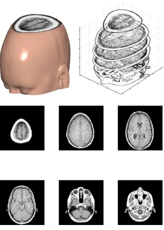
1.1 Noisy MR image. . . 3
1.2 Motivation of 3D matching. . . 4
1.3 Examples of 3D models. . . 5
1.4 3D object matching diagram. . . 6
1.5 Topological equivalence of coffee cup and doughnut. . . 7
2.1 Image differential operators. . . 15
2.2 A facial image and its graph. . . 16
2.3 Image denoising as surface evolution. . . 17
2.4 Parametric representation of a surface. . . 18
2.5 Illustration of the Gauss map. . . 18
2.6 Triangle meshes. . . 20
2.7 Barycentric triangulation. . . 21
2.8 Volumetric surface. . . 22
3.1 Block diagram of image denoising process. . . 25
3.2 Total variation. . . 28
3.3 Anisotropic Lagrangians. . . 33
3.4 Image evolution under flows. . . 34
3.5 Huber function. . . 36
3.6 Huber influence function and its smooth version. . . 38
3.7 Log-Cauchy filtering: (a) contaminated image, (b) filtered image. . . 39
3.8 Visual comparison of some variational integrands . . . 42
3.9 Improved entropic Lagrangian. . . 43
3.10 Filtering results for Gaussian noise. . . 45
3.11 Filtering results for Laplacian noise. . . 46
4.1 Nondegenerate singular points. . . 55
4.2 Degenerate singularity: cusp point/curve . . . 56
4.3 A 3-D object and the critical points of its height function. . . 57
5.1 A 3-D object and the critical points of its height function. . . 64
5.2 Reeb graph representation of a torus. . . 65
5.3 (a) Self-shadow and cast shadow, (b) illumination of a Lambertian surface. . . 66
5.4 (a) Shading image, (b) gradient vector field, (c) shading normal field . . . 67
5.5 Reeb graph of the heart model. . . 72
5.6 Reeb graph of the hand model. . . 72
6.1 Distance between two arbitrary centroids of a 3D camel. . . 77
6.2 Block-diagram of the proposed methodology. . . 78
6.3 Reeb graph representation . . . 80
6.4 Reeb graph of the hand model. . . 81
6.5 D2 shape distribution of an ellipsoid. . . 82
6.6 Euclidean vs. geodesic distance on a nonlinear manifold. . . 84
6.7 Effect of the bandwidth parameter h. . . 86
6.8 Geodesic shape distribution algorithm. . . 87
6.9 (a) 3D tank model, and its (b) geodesic shape distribution. . . 87
6.10 Robustness and invariance. . . 88
6.11 Robustness and invariance (cont.). . . 89
6.12 (a) 3D plot and (b) contour plot of the Jensen-Shannon divergence. . . 90
6.13 Illustration of geodesic shape statistical manifold. . . 93
6.14 First set of experiments: 3D airplanes. . . 94
6.15 Second set of experiments: 3D tanks. . . 95
6.16 Third set of experiments: 3D models and their geodesic shape distributions. . . 97
6.17 Fourth set of experiments: 3D models and their geodesic shape distributions. . . 98
7.1 Definition of a 2-manifold. . . 102
7.2 Critical points. . . 104
7.3 A 3-D object and the critical points of its height function. . . 106
7.4 Illustration of the height function. . . 108
7.5 Surface immersed in water. . . 110
7.6 Reeb graph representation . . . 111
7.7 Illustration of Ma and La. . . 112
7.8 Evolution ofMa asachanges. . . 113
7.9 handle decomposition. . . 114
7.10 Illustration of the distance function. . . 116
7.11 Embedding of a 3D airplane into a sphere. . . 117
7.12 Distance function defined on a torus. . . 118
7.13 Distance function defined on a torus (cont.). . . 118
7.14 Distance function defined on a dimple. . . 119
7.15 Isocontours of 3D real data. . . 119
Chapter
1
Introduction
With the increasing use of scanners to create images, there is a rising need for robust image denoising to remove inevitable noise in the measurements. Even with high-fidelity scanners, the acquired images are invariably noisy, and therefore require filtering. For instance, images extracted from volume data, that is obtained by MRI or CT devices, often contain amounts of noise that must be removed before further processing. Removing noise while preserving the details is, however, no trivial matter since sharp features are often blurred and therefore efficient image denoising techniques are needed. In this thesis, we propose robust variational models for image denoising by solving partial differential equations. The core idea behind our proposed approaches is to use geometric insight in helping construct regularizing functionals and avoiding a subjective choice of a prior in maximum a posteriori estimation. Using tools from robust statistics and information theory, we show that we can extend this strategy and develop two gradient descent flows for image denoising with a demonstrated performance.
The major part of this thesis is devoted to a joint exploitation of geometry and topology of objects for as parsimonious as possible representation of objects and its subsequent application in object classification and recognition. The key idea consists of capturing geometry along all topologically homogeneous parts of an object by way of level curves superimposed on a Reeb graph usually extracted by way of the object critical points. A Reeb graph is a topological representation of the connectivity of a surface between critical points which represent the nodes of the graph, and the edges of the graph represent the connected components of the surface. Specifically, given a function defined on a surface or 2-manifold, a Reeb graph may be used to track its connected
components as the pre-image of the function. For the example of using a height function, the Reeb graph would contain nodes for each of the contours for each level set generated by the height function. The resulting skeletal representation, however, is not rotationally invariant due to the rotational non-invariance of the height function. We propose a new methodology called
geodesic shape distributionthat lifts this limitation and which we apply to three-dimensional object matching. The central idea is to encode a 3D shape into a 1D geodesic shape distribution. Object matching is then achieved by calculating an information-theoretic measure of dissimilarity between resulting probability distributions. That is, the dissimilarity computations are carried out in a low-dimensional space of geodesic shape distributions.
1.1
Framework and motivation
1.1.1 Image denoising
Image denoising refers to the process of recovering an image contaminated by noise. The challenge of the problem of interest lies in faithfully recovering the original image from the observed image, and furthering the estimation by making use of any prior knowledge/assumptions about the noise process. The problem of image denoising has been addressed using a number of different techniques including wavelets [49], order statistics based filters [17], PDE-based algorithms [30, 76], and varia-tional approaches [26,27,6]. In particular, a large number of PDE-based methods have particularly been proposed to tackle the problem of image denoising [4,23,25] with a good preservation of edges. Much of the appeal of PDE-based methods lies in the availability of a vast arsenal of mathematical tools which at the very least act as a key guide in achieving numerical accuracy as well as stability. Partial differential equations or gradient descent flows are generally a result of variational problems using the Euler-Lagrange principle [36].
1.1 Framework and motivation 3
3D object MR Image Noisy Image
Figure 1.1: Noisy MR image.
1.1.2 Object recognition
Three-dimensional objects consist of geometric and topological data, and their compact represen-tation is an important step towards a variety of computer vision applications including indexing, retrieval, and matching in a database of 3D models. The latter will be the focus of Chapter 6, and the motivation behind considering 3D objects is illustrated in Figure 1.2.
3D models do not depend on the configuration of cameras, light sources, or surrounding objects. As a result, they do not contain reflections, shadows, occlusions, projections, or partial objects, which in turn greatly simplifies finding matches between objects of the same type. For example, it is plausible to expect that the 3D model of a Boeing747 contains exactly four engines. In contrast, any 2D image of this Boeing747 may contain fewer than four engines (if some of the engines are occluded), or it may contain “extra engines” appearing as the result of shadows.
In other respects, representing and processing 3D models is more complicated than for sampled multimedia data. The main difficulty is that 3D surfaces rarely have simple parameterizations. Since 3D surfaces can have arbitrary topologies, many useful methods for analyzing other media (e.g., Fourier analysis) have no obvious analogs for 3D surface models. Moreover, the dimension-ality is higher, and this makes searches for pose registration, feature correspondences, and model parameters more difficult.
• 2D provides the grayscale/color information in the plane: lost of depth information
• e.g.: 2D images of F-16s and MiG-23s look very similar, but in 3D are different
• 3D is much more effective for recognition and dis-play
• 3D applications: industry, medicine, search, video games and cinema
Figure 1.2: Motivation of 3D matching.
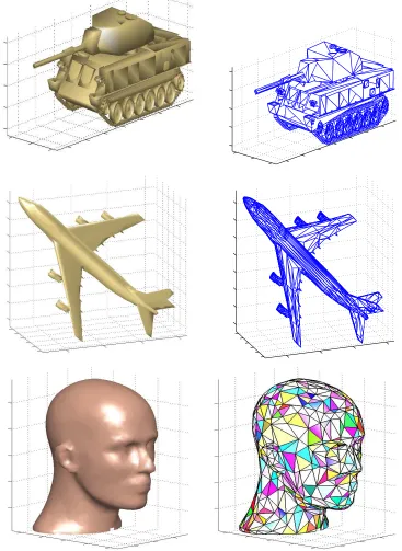
3D models, and a small subset of our large database is depicted in Figure 1.3. We collected several hundred models which consist of military objects, human body parts, animals and other objects.
There are two major techniques for 3D object recognition: feature-based and global methods as depicted in Figure 1.4. Most three-dimensional shape matching techniques proposed in the literature of computer graphics, computer vision and computer-aided design are based on geometric representations which represent the features of an object in such a way that the shape dissimilarity problem reduces to the problem of comparing two such object representations. Feature-based methods require that features be extracted and described before two objects can be compared.
1.1 Framework and motivation 5
3D Object Recognition
Global Methods
Feature−based Methods
Shape Signature
Signature Matching
Graph Representation
Graph Matching
Figure 1.4: 3D object matching diagram.
1.1.3 Joint exploitation of geometry and topology
1.1 Framework and motivation 7
≡
Figure 1.5: Topological equivalence of coffee cup and doughnut.
geometric aspects of the surface, for example, the geodesic distance is a global geometric measure. This interplay of geometry and topology is inherent in the discrete nature of the surfaces used in the field of computer graphics where great care is taken with the geometry of a surface, as the geometry plays such an important role in determining the appearance of a surface. Although a coffee cup is topologically equivalent to a doughnut, geometrically the shapes differ as shown in Figure 1.5. And the difference in their appearance matters greatly when the goal is to accurately represent the appearance of real world objects. Thus, a great deal of work in computer graphics has focused on geometric aspects of a surface, including geometry acquisition, geometry simplification, geometry smoothing and geometry compression. However, there is a direct relationship between the topology and the geometry of a surface that cannot be ignored. Alternatively, many mathematicians and computational topologists are concerned with studying purely topological properties of a surface. This thesis takes a combined approach and identifies and localizes topological features within a surface by mixing topological and geometrical approaches.
1.2
Contributions
The contributions of this thesis are as follows:
Robust and efficient variational filters for image denoising: Using the theoretical fun-damentals of robust statistics, a variational filter referred to as a Huber gradient descent flow is proposed. It is a result of optimizing a Huber functional subject to some noise constraints, and it takes a hybrid form of a total variation diffusion for large gradient magnitudes and of a linear diffusion for small gradient magnitudes. Using the gained insight, and as a fur-ther extension, we propose an information-theoretic gradient descent flow which is a result of minimizing a functional that is a hybrid between a negentropy variational integral and a total variation. Illustrating experimental results demonstrate a much improved performance of the approach in the presence of Gaussian and heavy tailed noise.
A Topological Variational Model for Image Singularities: Image singularities are promi-nent landmarks and their detection, recognition, and classification is a crucial step in image processing and computer vision. Such singularities carry important information for further operations, such as image registration, shape analysis, motion estimation, and object recog-nition. In this thesis, we propose a topological gradient descent flow for image singularities. The approach is expressed in the higher order variational framework as a minimizer of a vari-ational integral involving the gradient and the Hessian matrix of the height function defined on a manifold. We demonstrate through numerical simulations the power of the proposed technique in preserving image singularities.
1.3 Thesis overview 9
framework, and its close relationship to the shading problem is also highlighted. Some numer-ical simulations with synthetic and real 3D data are provided to demonstrate the potential of object singularities in topological modeling.
Geodesic Object Representation and Recognition: We propose a shape signature that captures the intrinsic geometric structure of 3D objects. The primary motivation of the proposed approach is to encode a 3D shape into a one-dimensional geodesic distribution function. This compact and computationally simple representation is based on a global geodesic distance defined on an object surface, and takes the form of a kernel density estimate. To gain further insight into the geodesic shape distribution and its practicality in 3D computer imagery, some numerical experiments are provided to demonstrate the potential and the much improved performance of the proposed methodology in 3D object matching. This is carried out using an information-theoretic measure of dissimilarity between probabilistic shape distributions.
Distance Function-based Object Recognition: We introduce a topological approach to object recognition using a distance function. Similarly to the height function strategy which consists of reconstructing surface from its cross-sections, the key idea behind using a distance function is that a surface may be reconstructed from its intersections with concentric spheres centered at the centroid of the underlying surface. As the distance function traverses the surface and the number of intersecting contours changes for various distances (i.e. radii of concentric spheres) from the barycenter point, the topology of the surface varies as well.
1.3
Thesis overview
The organization of this thesis is as follows:
In Chapter 3, we present a variational approach to maximum a posteriori estimation MAP estimation. The key idea behind this approach is to use geometric insight in helping construct regularizing functionals and avoiding a subjective choice of a prior in MAP estimation. Using tools from robust statistics and information theory, we show that we can extend this strategy and develop two gradient descent flows for image denoising with a demonstrated performance.
In Chapter 4, we propose a geometric/topological variational model to preserve degenerate image singularities. Such singularities carry important information for a variety of image processing and computer vision operations, such as image registration, shape analysis, object recognition, etc. The approach is expressed in the higher order variational framework, and it is based on a variational integral involving the gradient and the Hessian matrix of the height function defined on a manifold.
Chapter 5 is devoted to a formulation of object singularities in a Morse theoretic setting. Then, we analyze the Reeb graph representation in the shading problem framework, and we derive some relevant theoretical properties of the height function in the light direction of an illuminated 3D object. In addition, we prove that such a height function is closely related to the generalized bas-relief transformation.
1.4 Publications 11
matching can then be carried out by dissimilarity measure calculations between geodesic shape distributions, and is in addition computationally efficient and inexpensive.
Chapter 7 is devoted to the distance function-based approach to topological modeling using Morse theory. Despite the theoretical nature of the results presented in this Chapter, the key idea if to identify and encode regions of topological interest of 3D object in the Morse-theoretic framework. The main motivation behind using the distance function is its rotation invariance which makes it more adapted to object recognition than the Morse height function. We prove that a surface may be reconstructed from its intersections with concentric spheres centered at the barycenter of the underlying surface. The topological changes in the surface occur as we increase the value of the sphere radius. At singular points, the level curves of the distance function may split or merge which indicate topological changes. We also show that when a surface is embedded in a sphere, the height function and the distance function are equivalent in a Morse-theoretic setting, that is both functions have the same singularities.
In theConclusionsChapter, we summarize the contributions of this thesis, and we propose several future research directions that are directly or indirectly related to the work performed in this thesis.
1.4
Publications
A. Ben Hamza, Hamid Krim, and Gozde Unal, “Unifying probabilistic and variational esti-mation,”IEEE Signal Processing Magazine, vol. 19, no. 5, pp. 37-47, September 2002.
Yun He, A. Ben Hamza, and Hamid Krim, “A generalized divergence measure for robust image registration,”IEEE Transactions on Signal Processing, vol. 51, no. 5, pp. 1211-1220, May 2003.
A. Ben Hamza and Hamid Krim, “A Variational approach to maximum a posteriori estimation for image denoising,” Lecture Notes in Computer Science, vol. 2134, pp. 19-34, 2001.
A. Ben Hamza and Hamid Krim, “Geodesic object representation and recognition,” Lecture Notes in Computer Science, to appear 2003.
A. Ben Hamza and Hamid Krim, “Image registration and segmentation by maximizing Jensen-Renyi divergence,”Lecture Notes in Computer Science, vol. 2683, pp. 147-163, 2003.
A. Ben Hamza and Hamid Krim, “Robust environmental image denoising,”ISI International Conference on Environmental Statistics and Health, 2003.
A. Ben Hamza and Hamid Krim, “Robust influence functionals for image filtering,” Proc. IEEE International Conference on Image Processing, Barcelona, Spain, 2003.
A. Ben Hamza and Hamid Krim, “A topological skeleton of illuminated manifolds,” Proc. IEEE International Conference on Image Processing, Barcelona, Spain, 2003.
A. Ben Hamza and Hamid Krim, “Jensen-Renyi divergence measure: theoretical and compu-tational perspectives,”Proc. IEEE International Symposium on Information Theory, 2003.
A. Ben Hamza and Hamid Krim, “A topological variational model for image singularities,”
Proc. IEEE International Conference on Image Processing, Rochester, NY, 2002.
Chapter
2
Background
This thesis addresses the application of computational geometry and topology algorithms to images and three-dimensional surfaces. The following background material is presented to provide context for this work. First, a representation of images in the continuous domain is presented along with some basic differential operators used throughout this work. Then, a discussion of the various surface representations of three-dimensional objects is presented.
2.1
Continuous representation of images
In the variational setting, an image is usually defined in the continuous domain which enjoys a large arsenal of analytical tools, and hence offers a greater flexibility. An image is therefore defined as a real-valued function u: Ω→ R, where Ω is a nonempty, bounded, open set in the real plane
R2 (usually Ω is a rectangle in R2).
2.1.1 Differentiability of images
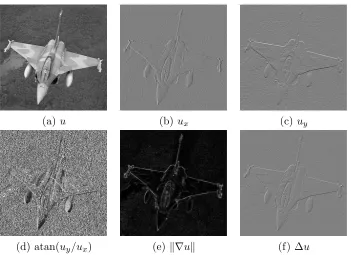
A pixel location in Ω is denoted byx= (x, y), and the gradient ofu is denoted by∇u= (ux, uy)T,
whereux and uy are the first-order partial derivatives with respect to x and y respectively. These
derivatives are illustrated in Figures 2.1(b) and (c). In image analysis, the image gradient defines the orientation of an edge at a given image point. The gradient orientation or directionθ= atan(uy/ux)
gives the orientation of the edge as shown in Figure 2.1(d). An edge in an image is a contour across which the image intensity changes abruptly. Image edges are usually considered to be discontinuities
of the image intensity function. The gradient magnitude k∇uk= qu2
x+u2y gives the strength of
the edge, and it defines an edge image whose pixels are bright only near an edge as depicted in Figure 2.1(e). To detect edges of any orientation, first we compute the gradient of the image, then compute the gradient magnitude at every pixel, and then label as “edge pixels” all pixels whose gradient magnitude is above a pre-determined threshold.
The Hessian matrix∇2uof an imageuis defined as the matrix of second-order partial derivatives
∇2u=
uxx uxy
uxy uyy ,
and its Laplacian is defined as the divergence of the gradient or the trace of the Hessian matrix
∆u=∇ ·(∇u) = div(∇u) =uxx+uyy= Tr(∇2u).
Another way to detect edges is to use zero-crossing of the Laplacian which crosses zero in the neighborhood of an edge, and this technique can be used without relying on a threshold. The Laplacian image is depicted in Figure 2.1(f).
The Hessian matrix of an image consists of three termsuxx,uyy anduxy. The Laplacian ignores
the third term and returns the average value of the second derivative when taking every orientation into account. While the Laplacian ignores one of them and considers every possible orientation at once, the Hessian takes all three terms into account and is orientation-dependent. The largest eigenvalue of the Hessian determines the orientation along which the second derivative is maximal, while the smallest eigenvalue of the Hessian returns the minimum of the second derivative.
2.2
Three-dimensional surfaces
2.2 Three-dimensional surfaces 15
(a) u (b)ux (c)uy
(d) atan(uy/ux) (e)k∇uk (f) ∆u
Figure 2.1: Image differential operators.
the surface appears to be nearly flat. The world we live on is an excellent example of a 2-manifold. Manifolds are a preferable surface representation because the surface can be divided into regions calledchartswhich allow 2-manifolds embedded in 3D to be flattened into a two dimensional domain (through parametrization). Surfaces used in computer graphics are typically oriented, this refers to the fact that the surface has two sides. For example, a sphere has two sides, while a Mobius strip has only one side. Another attribute of surfaces is whether the surface is closed or with boundary. This refers to the number of open boundary components of a surface. For example, an egg shell is closed but once it has been cracked open, it becomes a surface with boundaries.
2.2.1 Image graph
To apply and benefit from the tools of geometry in image analysis, it is convenient to consider the graph of an imageuwhich is a surface (2-dimensional manifold)M⊆R3 defined asM={(x, y, z) :
Figure 2.2: A facial image and its graph.
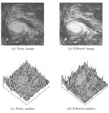
and its surface representation are depicted in Figure 2.2.
Inspired by this surface representation, the image denoising problem may be viewed as surface smoothing. This may be carried out by minimizing an energy functional with regularization terms that evolve the noisy surface to the optimal solution as depicted in Figure 2.3.
In order to allow partial differentiation and consequently all the features of differential calculus onM, we need to consider a smooth imageu, that is has continuous partial derivatives of all orders, so that the manifold M is differentiable. Thus the study of this differential manifold involves topology, since differentiability implies continuity. A common way to smooth an image u is to embed it into a family of images known as scale-space image. For example, a Gaussian scale-space image which is the result of convolving an image with the bivariate Gaussian density. A parametric representation of M is the Monge patch defined by r : Ω→ M such that r(x, y) = (x, y, u(x, y)). Note that the patch r covers all M, that is, r(Ω) =M, and it is regular, that is, rx×ry 6= 0 or
equivalently, the Jacobian matrix ofrhas rank 2. Figure 2.4 illustrates a parametric representation of a surface.
2.2 Three-dimensional surfaces 17
(a) Noisy image (b) Filtered image
(c) Noisy surface (d) Filtered surface
Figure 2.3: Image denoising as surface evolution.
smooth projectionπ : Ω×R→Ω, that is r−1 =π|M.
Let p∈M, then there exists (x, y)∈Ω such that p=r(x, y). Hence, the unit normalN toM is given by
N(p) =N(r(x, y)) = rx×ry
krx×ryk =
(−ux,−uy,1) q
1 +u2
x+u2y
. (1)
The unit normal is the most elementary differential characteristics of a surface and determines the tangent planeTpM at a surface point p=r(x, y). The tangent plane can be defined as the set of
.
.
PSfrag replacements r
(x, y)-plane
(x, y)
surface M
y
x
ry
rx
r(x, y)
N
1
Figure 2.4: Parametric representation of a surface.
normal is well-defined everywhere, and therefore the image graph M is orientable. For notational convenience, the unit normal can be viewed as a mappingg : Ω→S2, called Gauss map of r and
is defined as g(x, y) =N(r(x, y)), where S2 ={p ∈R3 :kpk = 1} is the unit sphere. Note that
g(x, y) denotes the values of the unit Gauss map at p=r(x, y) as illustrated in Figure 2.5.
Gauss map
.
.
.
.
M
S2
N(p)
N(p) p
2.2 Three-dimensional surfaces 19
2.2.2 Triangle mesh
In computer graphics, 3D objects are usually represented as a triangle mesh M = (V,T), where
V = {v1, . . . ,vm} is the set of vertices, and T = {T1, . . . , Tn} is the set of triangles. Triangle
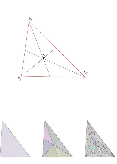
meshes are used so frequently to represent surfaces in the discrete domain that most computer graphics hardware is optimized to render triangles. Example of triangle meshes are depicted in Figure 2.8. For triangulation, we use the barycentric subdivision illustrated in Figure 2.7. This technique consists in introducing a new vertex at the center of each triangle and a new vertex at the midpoint of each edge and drawing edges from the centroid of the triangle to each of the new midpoint vertices and to the original vertices.
2.2.3 Scalar volume and isosurface
2.2 Three-dimensional surfaces \tex[B][B]{$v_1$ 21
Chapter
3
Robust Variational Image Denoising
In this chapter, we present a variational approach to MAP estimation [6, 7]. The core idea behind this approach is to use geometric insight in helping construct regularizing functionals and avoiding a subjective choice of a prior in MAP estimation [8]. Using tools from robust statistics and infor-mation theory, we show that we can extend this strategy and develop two gradient descent flows for image denoising with a demonstrated performance [8, 9].
3.1
Introduction
In recent years, variational methods and partial differential equations (PDE) based methods [57, 61,1,65,2,74] have been introduced to explicitly account for intrinsic geometry to address a variety of problems including image segmentation, mathematical morphology, motion estimation, image classification, and image denoising [56, 62, 30, 47, 66, 4]. The latter will be the focus of the present chapter. The problem of signal/image denoising has been addressed using a number of different techniques including wavelets [49], order statistics based filters [17], PDE-based algorithms [30, 76], and variational approaches [26, 27, 6]. In particular, a large number of PDE-based methods have particularly been proposed to tackle the problem of image denoising [4, 23, 25] with a good preservation of edges. Much of the appeal of PDE-based methods lies in the availability of a vast arsenal of mathematical tools which at the very least act as a key guide in achieving numerical accuracy as well as stability. Partial differential equations or gradient descent flows are generally a result of variational problems using the Euler-Lagrange principle [36]. One popular variational
technique used in image denoising is the total variation based approach. It was developed in [65] to overcome the basic limitations of all smooth regularization algorithms, and a variety of numerical methods have also recently been developed for solving total variation minimization problems [43,24]. In the next section, a general formulation of signal/image denoising problem is stated. In Section 3.3, we briefly recall the MAP estimation technique, and in Section 3.4 we formulate the problem of MAP estimation in the calculus of variations setting. Section 3.5 is devoted to a robust variational formulation using concepts borrowed from robust estimation, followed by a probabilistic interpretation of the nonlinear anisotropic diffusion in the the order statistics framework. In Section 3.6, information-theoretic variational flows based on the differential entropy are proposed. In Section 3.7, we provide experimental results to demonstrate a much improved performance of the proposed gradient descent flows in image denoising. Finally, some conclusions and discussions are included in Section 3.8.
3.2
Problem statement
In all real applications, measurements are perturbed by noise. In the course of acquiring, transmit-ting or processing a digital image for example, the noise-induced degradation may be dependent or independent of data. The noise is usually described by its probabilistic model, e.g., Gaussian noise is characterized by two moments. Application-dependent, a degradation often yields a resulting signal/image observation model, and the most commonly used is the additive one,
u0 =u+η, (1)
where the observed image u0 includes the original signal u and the independent and identically
distributed (i.i.d) noise processη.
Image denoising refers to the process of recovering an image contaminated by noise (see Fig-ure 3.1). The challenge of the problem of interest lies in faithfully recovering the underlying sig-nal/imageufromu0, and furthering the estimation by making use of any prior knowledge/assumptions
3.3 MAP estimation: model-based approach 25
PSfrag replacements
η
u + u+η
prior denoising
ˆ u
Figure 3.1: Block diagram of image denoising process.
3.3
MAP estimation: model-based approach
In a probabilistic setting, the image denoising problem is usually solved in a discrete domain, and in this case an image is expressed by a random matrix u = (uij) of gray levels. To account for
prior probabilistic information we may have for u, a technique of choice is that of a maximum a posteriori estimation. Denoting by p(u) the prior distribution for the unknown imageu, the MAP estimator is given by
ˆ
u= arg max
u {logp(u0|u) + logp(u)}, (2)
wherep(u0|u) denotes the conditional probability of u0 given u.
A general model for the prior distribution p(u) is that of a Markov random field (MRF) which is characterized by its Gibbs distribution given by [33]
p(u) = 1
Z exp
½
−Fλ(u)
¾
,
of physical systems. F is called theenergy functionand has the form F(u) =Pc∈CVc(u), whereC
denotes a set of cliques (i.e. set of connected pixels) for the MRF, and Vc is a potential function
defined on a clique. We may define the cliques to be adjacent pairs of horizontal and vertical pixels. Note that for large λ, the prior probability becomes flat, and for small λ, the prior probability exhibits sharp modes.
Markov random fields have been extensively used in computer vision particularly for image restoration, and it has been established that Gibbs distributions and MRF’s are equivalent ( e.g. see [33]). In other words, if a problem is defined in terms of local potentials then there is a simple way of formulating the problem in terms of MRF’s. If the noise process η is i.i.d. Gaussian, then we have
p(u0|u) =Kexp
µ
−|u−u0|
2
2σ2
,
whereKis a normalizing positive constant,σ2is the noise variance, and|·|stands for the Euclidean norm or for the absolute value in the case of a scalar. Thus, the MAP estimator in (2) yields
ˆ
u= arg min
u ½
F(u) +λ
2|u−u0|
2
¾
. (3)
Image estimation using MRF priors has proven to be a powerful approach to restoration and reconstruction of high-quality images. Its major drawback, besides its computational load, is the difficulty in systematically selecting a practical and reliable prior distribution. The Gibbs prior parameterλis also of particular importance since it controls the balance of influence of the Gibbs prior and that of the likelihood. If λ is too small, the prior will tend to have an over-smoothing effect on the solution. Conversely, if it is too large, the MAP estimator may be unstable and it reduces to the maximum likelihood solution asλgoes to infinity. Another difficulty in using a MAP estimator is the non-uniqueness of the solution when the energy functionF is not convex.
3.4
A variational approach to MAP estimation
3.4 A variational approach to MAP estimation 27
preserve high gradients in a geometric setting, or determine a worst case noise distribution in a sta-tistical estimation setting with a number of interpretations), and may not necessarily be tractably assessed by an objective and optimal performance measure. The formulation of such qualitative goals, is typically carried out by way of adapted functionals which upon being optimized, achieve the stated goal, e.g. a monotonically decreasing functional of gradient modifying a diffusion [61]. This approach is the so-called variational approach. It is commonly formulated in a continuous domain which enjoys a large arsenal of analytical tools, and hence offers a greater flexibility. An image is therefore defined as a real-valued functionu: Ω→R, and Ω is a nonempty, bounded, open set in R2 (usually Ω is a rectangle in R2). Throughout, x= (x
1, x2) denotes a pixel location in Ω,
and || · || denotes theL2-norm. While the ultimate overall objective in the aforementioned
formu-lation may coincide with that of a probabilistic formuformu-lation, namely the recovery of an underlying desired signalu, it is herein often implicit and embedded in an energy functional to be optimized. Generally, the construction of an energy functional is based on some characteristic quantity spec-ified by the task at hand (gradient for segmentation, Laplacian for smoothing, etc.). This energy functional is oftentimes coupled to a regularizing force/energy in order to rule out a great number of solutions and to also avoid any degenerate solution.
When considering the signal model (1), our goal may be succinctly stated as one of estimating the underlying image u based on an observation u0 and/or any potential knowledge of the noise
statistics to further regularize the solution. This yields the following fidelity-constrained optimiza-tion problem
min
u F(u)
s.t. ku−u0k2 =σ2
(4)
where F is a given functional which often defines, as noted above, the particular emphasis on the features of the achievable solution. In other words, we want to find an optimal solution that yields the smallest value of the objective functional among all solutions that satisfy the constraints. Using Lagrange’s theorem, the minimizer of (4) is given by
ˆ
u= arg min
u ½
F(u) +λ
2ku−u0k
2
¾
, (5)
practice, the parameter λis often estimated or chosena priori.
Equations (3) and (5) show a close connection between image recovery via MAP estimation and image recovery via optimization of variational integrals. One may in fact reexpress (3) in an integral form similar to that of (5).
A critical issue, however, is the choice of the variational integralF, which as discussed later, is often driven by geometric arguments. Among the better known functionals (also calledvariational integrals) in image denoising are the Dirichlet and the total variation integrals defined respectively as
D(u) = 1
2
Z
Ω|∇
u|2dx and T V(u) =
Z
Ω|∇
u|dx,
where ∇u denotes the gradient of the image u. The total variation method basically consists in finding an estimate ˆufor the original imageuwith the smallest total variation among all the images satisfying the noise constraintku−u0k2 =σ2, whereσis assumed known. Note that the parameter
λcontrols the trade-off between noise removal and detail preservation.
0 1 2 3 4
1 2 3 4
PSfrag replacements
u1
u2
u3
T V(u1) = 6 T V(u2) = 6 T V(u3) = 4
1
Figure 3.2: Total variation.
3.4 A variational approach to MAP estimation 29
success in image denoising, especially for denoising images with piecewise constant features while preserving the location of the edges exactly [23].
The Dirichlet and total variation functionals can be written is a generalized form given by
F(u) =
Z
Ω
F(|∇u|)dx, (6)
where F : R+ → R is a given smooth function called a variational integrand or Lagrangian [36]. Using (6), we hence define a functional
L(u) = F(u) + λ
2ku−u0k
2
=
Z
Ω
µ
F(|∇u|) + λ
2|u−u0|
2
dx, (7)
which by the formulation in (5) becomes
ˆ
u= arg min
u∈XL(u), (8)
whereXis an appropriate image space of smooth functions likeC1(Ω), or the spaceBV(Ω) of image functions with bounded variation, or the Sobolev space H1(Ω) = W1,2(Ω). Note that BV(Ω) is a
Banach space with the normkukBV =kukL1(Ω)+T V(u), while H1(Ω) is a Hilbert space with the
norm kuk2
H1(Ω)=kuk2+k∇uk2.
3.4.1 Properties of the optimization problem
A problem is said to be well-posed in the sense of Hadamard if (i) a solution of the problem exists, (ii) the solution is unique, (iii) and the solution is stable, i.e. depends continuously on the problem data. It isill-posedwhen it fails to satisfy at least one of these criteria. To guarantee the well-posedness of our minimization problem (8), the following result provides some conditions.
Proposition 3.1 Let the image space X be a reflexive Banach space, and let F be
(i) weakly lower semicontinuous, i.e. if for any sequence(uk)in X converging weakly tou, we have
F(u)≤lim infk→∞F(uk).
(ii) coercive, i.e. F(u)→ ∞ askuk → ∞.
such that L(ˆu) = infXL. Moreover, if F is convex and λ >0, then the optimization problem (8)
has a unique solution, and therefore it is stable.
Proof: From (i) and (ii) and the weak lower semicontinuity of the L2-norm, the functional L
is weak lower semicontinuous, and coercive, i.e. L(u)→ ∞ askuk → ∞. Let un be a minimizing sequence of L, i.e. L(un) → inf
XL. An immediate consequence of the
coercivity ofLis thatunmust be bounded. AsX is reflexive, thusun converges weakly to ˆu inX, i.e un*uˆ. Thus L(ˆu)≤lim inf
n→∞L(un) = infXL. This proves thatL(ˆu) = infXL.
It is easy to check that convexity implies weakly lower semicontinuity. Thus the solution of the optimization problem (8) exists and it is unique because the L2-norm is strictly convex. The
stability follows using the semicontinuity ofL and the fact thatun is bounded.
3.4.2 Numerical solution: gradient descent flows
To solve the optimization problem (8), a variety of iterative methods such as gradient descent [65], or fixed point method [43, 24] may be applied.
The first-order necessary condition to be satisfied by any minimizer of the functional L given by (7) is that its first variationδL(u;v) vanishes atu in direction ofv, that is
δL(u;v) = d
d²L(u+²v)
¯ ¯ ¯ ¯ ¯ ²=0
= 0, (9)
and a solutionu of (9) is called a weak extremalof L [36].
Using (7) and (9), we obtain the first variation δL(u;v) (see Appendix A for a proof)
δL(u;v) =
Z
Ω
½µ
F0(|∇u|)
|∇u| ∇u· ∇v
+λ(u−u0)v
¾ dx = − Z Ω ½ div µ
F0(|∇u|)
|∇u| ∇u
+λ(u−u0)
¾
v dx, (10)
for all v∈X.
3.4 A variational approach to MAP estimation 31
an Euler-Lagrange equation as a necessary condition to be satisfied by minimizers ofL. In mathe-matical terms, the Euler-Lagrange equation is given by
−div
µ
F0(|∇u|)
|∇u| ∇u
+λ(u−u0) = 0, in Ω, (11)
where “div” stands for the divergence operator. An imageu satisfying (11) is called anextremalof
L.
Note that|∇u|is not differentiable when∇u= 0 (e.g. flat regions in the imageu). To overcome the resulting numerical difficulties, we use the following slight modification
|∇u|²=
p
|∇u|2+²,
where²is positive sufficiently small.
Proposition 3.2 Let λ= 0, and S be a convex set of an image space X. If the Lagrangian F is nonnegative convex and of class C1, then every weak extremal of L is a minimizer of L onS.
Proof: The convexity of F yields
F(y)≥F(x) +F0(x)(y−x), ∀x, y∈R+. (12)
By assumption u is a weak extremal of L, ie. δL(u;v) = 0 for all v ∈ S. This implies that
F0(|∇u|) = 0. Therefore, using (12) we obtain
Z
Ω
F(|∇v|)dx≥
Z
Ω
F(|∇u|)dx.
This concludes the proof.
By further constrainingλ, we may be in a position to sharpen the properties of the minimizer, as given in the following.
Proof: Using (12), it follows that F(|∇u|)≥F(0). Thus the constant image is a minimizer of
L. Since S is convex, it follows that this minimizer is global.
Proposition 3.4 Let λ > 0, and S be a convex set of image space X. If the Lagrangian F is nonnegative strictly convex and of class C1, then an extremalu of L is the unique minimizer ofL
onS.
Proof: Sinceu7−→ λ2|u−u0|2 is strictly convex whenλ >0, then the functional L(u) is strictly
convex onS, that is
L(v)>L(u) +∇L(u)·(v−u).
By assumptionu is an extremal ofL, thusL(v)>L(u), for allv6=u.
Using the Euler-Lagrange variational principle, the minimizer of (8) may be interpreted as the steady state solution to the following nonlinear elliptic PDE calledgradient descent flow
ut= div(g(|∇u|)∇u)−λ(u−u0), in Ω×R+, (13)
where g(z) =F0(z)/z, withz >0, and assumed homogeneous Neumann boundary conditions. A numerical implementation of this partial differential equation is discussed in Appendix B.
3.4.3 Illustrative cases
The following examples illustrate the close connection between optimization problems of variational integrals and boundary value problems for partial differential equations in a no noise constraint case (i.e. setting λ= 0):
(a) Heat equation: ut= ∆u is the gradient descent flow for the Dirichlet variational integral D(u).
3.4 A variational approach to MAP estimation 33
(b) Perona-Malik (PM) equation: It has been shown in [77] that the PM diffusionut= div(g(|∇u|)∇u)
is the gradient descent flow for the variational integral
Fc(u) =
Z
Ω
Fc(|∇u|)dx,
with sample Lagrangians F1
c(z) = c2log ¡
1 +z2/c2¢ or F2
c(z) = c2 ¡
1−exp¡−z2/c2¢¢,
where z ∈ R+ and c is a tuning positive constant. These Lagrangians are depicted in Fig-ure 3.3.
0 1 2 3 4 5 6
0 0.2 0.4 0.6 0.8 1 1.2 1.4 1.6 1.8 2 PSfrag replacements
|∇u| F1
c(|∇u|) F2
c(|∇u|)
Figure 3.3: Anisotropic Lagrangians.
A minimization of such functionals encourages the smoothing of homogenuous/small gradient regions and the preservation of edges/high gradient regions. Note that ill-posedness of this formulation was addressed in a number of papers (e.g., see [77]). A result of applying the PM flow withFc1 to the original image in Figure 3.4(a) is illustrated in Figure 3.4(c). It is worth noting how the diffusion takes place throughout the homogeneous regions and not across the edges.
While limiting spurious oscillations, TV optimization preserves sharp jumps as is often encountered in “blocky” signals/images. Figure 3.4(d) illustrates the output of the TV flow.
(a) Original image (b) Heat flow
(c) Perona-Malik flow (d) TV flow
3.5 Robust variational approach 35
3.5
Robust variational approach
3.5.1 Robustness for unknown statistics
In robust estimation, for example, a case where even the noise statistics are not precisely known [42, 49] arises. In this case, a reasonable strategy would be to assume that the noise is a member of some set, or of some class of parametric families, and to pick the worst case density (least favorable, in some sense) member of that set, and obtain the best signal reconstruction for it. Huber’s
²-contaminated normal setP² is defined as [42]
P²={(1−²)Φ +²H : H∈ S},
where Φ is the standard normal distribution, S is the set of all probability distributions symmetric with respect to the origin and²∈[0,1] is the known fraction of “contamination”. Huber found that the least favorable distribution in P² which maximizes the asymptotic variance (or, equivalently,
minimizes the Fisher information) is Gaussian in the center and Laplacian in the tails. The transi-tion between the two depends on the fractransi-tion of contaminatransi-tion ², i.e., larger fractions correspond to smaller switching points and vice versa.
For the set P² of ²-contaminated normal distributions, the least favorable distribution has a
density function
fH(z) = ((1−²)/
√
2π) exp(−ρk(z)),
whereρk is the Huber M-estimator cost function (see Figure 3.5) given by
ρk(z) = z2
2 if|z| ≤k
k|z| − k
2
2 otherwise.
Here kis a positive constant determined by the fraction of contamination ²by the equation
2
µ
φ(k)
k −Φ(−k)
= ²
1−², (14)
where Φ is the standard normal distribution function and φ is its probability density function. It is clear thatρk is a convex function, quadratic in the center and linear in the tails as illustrated in
PSfrag replacements −k ρk ( z ) k z
Figure 3.5: Huber function.
Motivated by the robustness of the Huber M-filter in a probabilistic setting and its resilience to impulsive noise, we propose a variational filter which, when accounting for these properties, leads to the following energy functional
Rk(u) =
Z
Ω
ρk(|∇u|)dx.
Note that the Huber variational integral is a hybrid of the Dirichlet variational integral (ρk(|∇u|)∝
|∇u|2/2 ask→ ∞) and of the total variation integral (ρ
k(|∇u|)∝ |∇u|ask→0). One may check
that the Huber variational integral Rk : H1(Ω) → R+ is well defined, convex, and coercive. It
follows from Proposition 1 that the minimization problem ˆ
u= arg min
u∈H1(Ω)
½
Rk(u) +
λ
2ku−u0k
2
¾
= arg min
u∈H1(Ω)
Z
Ω
µ
ρk(|∇u|) +
λ
2|u−u0|
2
dx (15) has a solution. This solution is unique whenλ >0.
Proposition 3.5 The optimization problem (15) is equivalent to
ˆ
u= arg min
(u,θ)∈H1(Ω)×R
½ θ2 2 + Z Ω µ
k¯¯¯|∇u| −θ¯¯¯+λ
2|u−u0|
2
dx
¾
3.5 Robust variational approach 37
Proof: For z fixed, define Ψ(θ) = 12θ2 +k|z−θ| on R. It is is clear that Ψ is convex on
R. It follows that Ψ attains its minimum at θ0 such that Ψ0(θ0) = 0 and Ψ00(θ0) > 0, that is
θ0=k sign(z−k). Thus we have
Ψ(θ0) =
kz−k
2
2 ifz > k
z2
2 ifz=k
−kz−k
2
2 ifz <−k, and thereforeρk(z) = arg minθ∈RΨ(θ). This concludes the proof.
Using the Euler-Lagrange variational principle, a Huber gradient descent flow is obtained as
ut= div(gk(|∇u|)∇u)−λ(u−u0), in Ω×R+, (17)
wheregk is the Huber M-estimator weight function
gk(z) =
ρ0
k(z)
z =
1 if|z| ≤k k
|z| otherwise.
For large k, this flow yields an isotropic diffusion (heat equation whenλ= 0), and for smallk, it corresponds to total variation gradient descent flow (curvature flow when λ= 0).
It is worth pointing out that in the case of no noise constraint (i.e. setting λ= 0), the Huber gradient descent flow yields a robust anisotropic diffusion [20] obtained by replacing the diffusion functions proposed in [61] with robust M-estimator weight functions [42].
Recently, we proposed a smooth Huber variational integral [18] given by Φ(u) =
Z
Ω
ϕ(|∇u|)dx,
where the Lagrangianϕis defined as
ϕ(t)=
−c t ift≤ −a
(t+a)3/3−c t if−a < t <−b
(t2−b2)/2 + ((a−b)3+ 3bc)/3 if−b≤t≤b
−(t−a)3/3 +c t ifb < t < a
witha= 3/2,b= 1, andc= 5/4. Its derivativeϕ0 (also referred to as influence function in robust
statistics) is depicted in Figure 3.6. The Huber influence function, however, is not differentiable as shown in Figure 3.6. The differentiability of the influence function is of great importance since it implies the continuity of its first derivative which in turn implies the continuity of the confidence intervals in the data points. A more detailed description of the smooth Huber gradient descent flow will be reported elsewhere.
Huber smooth Huber
Figure 3.6: Huber influence function and its smooth version.
3.5.2 Perona-Malik equation: an estimation-theoretic perspective
In a similar spirit as above, one may proceed to justify the Perona-Malik equation from a specific statistical model. Assuming an imageu= (uij) as a random matrix with i.i.d. elements, the output
3.6 Information based functionals 39
the output of a Log-Cauchy filter is the solution to the following robust estimation problem [17]
min
θ X
i,j
log(c2+ (uij −θ)2) = min θ
X
i,j
Fc(uij−θ),
where the cost function Fc coincides with the Lagrangian function which yields the Perona-Malik
equation. Hence, in the probabilistic setting the Perona-Malik flow corresponds to the Log-Cauchy filter. Figure 3.7 illustrates the performance of the Log-Cauchy filter in removing heavy-tailed (impulsive) noise.
(a) (b)
Figure 3.7: Log-Cauchy filtering: (a) contaminated image with impulsive noise, (b) filtered image.
3.6
Information based functionals
3.6.1 Information theoretic approach
processu, and has been used with success in numerous image processing applications. The term is often associated with qualifying the selection of a distribution subject to some moments constraints (e.g. mean, variance, etc.), that is, the available information is described by way of moments of some known functionsmr(u) withr = 1, . . . , s. Indeed coupling the finiteness ofmr(u) for example
with the maximum entropy condition of the data suggests a most random model p(u) with the corresponding moments constraints as a most adapted model (equivalently minimizing negentropy see e.g. [48]).
min
u R
p(u) logp(u)du
s.t. Rp(u)du= 1
R
mr(u)p(u)du=µr, r= 1, . . . , s
(18)
Using Lagrange’s theorem, the solution of (18) is given by
p(u) = 1
Z exp ( − s X r=1
λrmr(u) )
, (19)
where λr’s are the Lagrange multipliers, and Z is a partition function. The resulting model p(u)
given by (19) may hence be used as a prior in a MAP estimation formulation.
3.6.2 Entropic gradient descent flow
Motivated by the good performance of the maximum entropy principle in image/signal analysis applications and inspired by its rationale, we may naturally adapt it to describe the distribution of a gradient throughout an image. Specifically, the large gradients should coincide with tail events of this distribution, while the small and medium ones representing the smooth regions, form the mass of the distribution. Towards that end, we write
H(u) =
Z
Ω
H(|∇u|)dx=
Z
Ω|∇
u|log|∇u|dx.
whereH(z) =zlog(z), z≥0. Note that −H(z)→0 as z→0. It follows from the inequalityzlog(z)≤z2/2 that
|H(u)| ≤
Z
Ω|∇
3.6 Information based functionals 41
where k · kH1(Ω) denotes the H1-norm. Thus the negentropy variational integral H: H1(Ω)→ R
is well defined. Note also that the inequality zlog(z) ≤z2/2 implies H(u) ≤ D(u), where D(u) is the Dirichlet integral. One may check that the Lagrangian H is strictly convex, and coercive, i.e.
H(z)→ ∞as|z| → ∞. The following result follows from Proposition 1.
Proposition 3.6 Let λ >0. The minimization problem
ˆ
u= arg min
u∈H1(Ω)
½
H(u) +λ
2ku−u0k
2
¾
= arg min
u∈H1(Ω)
Z
Ω
µ
|∇u|log|∇u|+λ
2|u−u0|
2
dx
has a unique solution provided that |∇u| ≥1.
Calling upon the Euler-Lagrange variational principle again, the following entropic gradient descent flow results
ut= div µ
1 + log|∇u|
|∇u| ∇u
−λ(u−u0), in Ω×R+,
with homogeneous Neumann boundary conditions. In addition, this energy spread of the gradient energy may be related to that sought by the total variation method, which in contrast allows for additional higher gradients.
Proposition 3.7 Let u be an image. The negentropy variational integral and the total variation satisfy the following inequality
H(u)≥T V(u)−1.
Proof: Since the negentropy H is a convex function, the Jensen inequality yields
Z
Ω
H(|∇u|)dx ≥ H
µZ
Ω|∇
u|dx
= H³T V(u)´ = T V(u) logT V(u),
and using the inequality zlog(z)≥z−1 for z≥0, we conclude the proof.
(i) If |∇u| ∈[0, e] thenH(u)≤T V(u) (ii) If|∇u| ∈(e,∞) thenH(u)> T V(u)
(iii) If |∇u| ∈(ek−1,∞) andk≥2 then H(u)≤ R
k(u),
whereeis the Euler number (e= limn→∞(1 + 1/n)n≈2.71).
0 1 2 3 4 5 6
−2 0 2 4 6 8 10 12 14
Entropy Total Variation Huber
PSfrag replacements
|∇u|
F
(
|∇
u
|
)
Figure 3.8: Visual comparison of some variational integrands
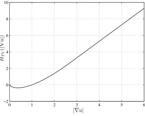
3.6.3 Improved entropic gradient descent flow
To summarize and for a comparison sake, we show in Figure 3.8 the behavior of the variational integrands we have discussed in this paper. It can be readily shown [6] that a differentiable hybrid functional between the negentropy variational integral and the total variation may be defined as
HT V(u) =
H(u) if|∇u| ≤e
2 T V(u)−meas(Ω)e otherwise,
3.6 Information based functionals 43
coercive. It follows from Proposition 1 that the minimization problem
ˆ
u= arg min
u∈H1(Ω)
½
HT V(u) +
λ
2ku−u0k
2
¾
(20)
has a unique solution provided thatλ >0.
Figure 3.9 depicts the improved entropic Lagrangian HT V :R+→Rdefined as
HT V(z) =
zlog(z) ifz≤e
2z−e o.w.
Using the Euler-Lagrange variational principle, it follows that the improved entropic gradient descent flow is given by
ut=∇ · µ
H0
T V(∇u|)
|∇u| ∇u
−λ(u−u0), in Ω×R+, (21)
with homogeneous Neumann boundary conditions.
0 1 2 3 4 5 6
−2 0 2 4 6 8 10 PSfrag replacements
|∇
u
|
H T V ( |∇ u | )