DOI 10.1007/s10845-014-0908-5
A method for a robust optimization of joint product
and supply chain design
Bertrand Baud-Lavigne · Samuel Bassetto · Bruno Agard
Received: 10 September 2013 / Accepted: 21 March 2014 © Springer Science+Business Media New York 2014
Abstract This paper proposes a method for finding a robust solution to the problem of joint product family and sup-ply chain design. Optimizing product design and the supsup-ply chain network at the same time brings substantial benefits. However, this approach involves decisions that can gener-ate uncertainties in the long term. The challenge is to come up with a method that can adapt to most possible environ-ments without straying too far from the optimal solution. Our approach is based on the generation of scenarios that correspond to combinations of uncertain parameters within the model. The performance of designs resulting from these scenario optimizations are compared to the performance of each of the other design scenarios, based on their probability of occurrence. The proposed methodology will allow practi-tioners to choose a suitable design, from the most profitable to the most reliable.
Keywords Robust design·Supply chain·Product family· Mixed linear programming
Introduction
Most companies function in a complex and unstable envi-ronment, which makes accurate forecasting difficult. At the same time, staying competitive requires keeping production B. Baud-Lavigne·S. Bassetto·B. Agard (
B
)CIRRELT, Département de Mathématiques et Génie Industriel, École Polytechnique de Montréal, C.P. 6079, succ. Centre-Ville, Montreal, Québec H3C 3A7, Canada
e-mail: [email protected] B. Baud-Lavigne
e-mail: [email protected] S. Bassetto
e-mail: [email protected]
costs to a minimum. Optimization offers a solution to this dilemma, however it calls for long term decision making based on market forecasts. How can practitioners deal with fluctuations in parameters, such as demand, the price of raw materials, and transportation costs, in their effort to optimize a supply network?
It had once been thought that increasing the level of com-monality in the platform product would provide the neces-sary leverage to reduce production and distribution costs on a large product family (Jiao et al. 2007;Wie et al. 2007).
This paper extends the joint product and supply chain design model proposed byBaud-Lavigne et al.(2011) with a robust design methodology. We first present the model, and then explain and discuss the concept of robustness in this context. In “Robust methodology for joint product and supply chain design” section, we propose our robust design methodology, and apply it in “Experiments to illustrate the methodology” section in an academic case study.
The state of the art
Simultaneous product and supply chain design
After decades of research on supply network design, prac-titioners have integrated mathematical methods into supply chain optimization (Shapiro 2001), and the emphasis must now move to cost reduction and the fulfillment of customer needs. The benefits of simultaneous product and supply chain design has been highlighted byBaud-Lavigne et al.(2012). However, this approach, in which decisions on standardiza-tion are made for a product family through product optimiza-tion followed by supply chain optimizaoptimiza-tion, is now consid-ered to be sub optimal. Several modeling hypotheses have been studied recently as solutions to the problem of joint
product and supply chain design. From the perspective of customer needs and how they are met by functionalities, it is possible to model the problem with a generic bill of materials (Lamothe et al. 2006;Zhang et al. 2010;Shahzad and Hadj-Hamou 2013). In this approach, the composition of the entire product family is determined at the same time as the supply chain network is designed, in order to lower procurement, production, and distribution costs while maximizing profits. Modular product design has been studied bySchulze and Li (2009) andHadj Khalaf et al.(2010), who were looking at finding the right modules to allow specific final products to be manufactured at lower cost. The integration of complex bills of materials allows manufacturers to adapt to most indus-trial issues, but the models produced are difficult to solve. Scenario modeling, proposed byElMaraghy and Mahmoudi (2009), has made solving them easier, thanks to a limited number of decision variables and simple constraints. The difficulty is to itemize each combination of bills of materi-als, which can be considered as a combinatorial problem for complex products.Chen(2010) considers bills of materials with an unlimited number of levels and with substitution pos-sibilities. With this approach, modeling is flexible, as there are many decision variables. However, such models are also difficult to solve.
Robustness assessment in supply chain design
In this paper, we focus on classical robustness, which enables us to evaluate some behaviors of a system that are character-ized by uncertainty.
According to Klibi et al. (2010), there are three types of uncertainty: randomness, chance, and deep uncertainty. With randomness, the parameters are not known precisely, but rather as a range with some probabilities; with chance, there is a possibility that one or more unexpected events will occur; with deep uncertainty, it is impossible to determine what is possible. Robustness is a broad term in optimiza-tion, which can be applied to the mathematical model, the algorithm, or the solution. A model is robust when it can adapt to several configurations; a robust algorithm is aimed at finding a good solution (or an optimal one) in a minimum amount of time and in most cases. There are three types of solution robustness: classical robustness, responsiveness, and resilience. Classical robustness applies to a solution that gives good results without depending on the actual environment. For example,Pan and Nagi(2010) propose a supply chain design which deals with demand uncertainty and opportu-nities. Responsiveness measures the capacity of the supply chain to react appropriately when there is some randomness in the process (Parvaresh et al. 2012;Meepetchdee and Shah 2007). Resilience evaluates the ability of the organization to return to normal operation following a major breakdown (Childerhouse and Towill 2004).
We suggest two ways of dealing with randomness in sup-ply chain design optimization, using stochastic models or deterministic models. With the first option, the problem is modeled with stochastic parameters and solved with analyt-ical methods—see the review of this option provided by Pei-dro et al.(2009). For example, an optimization method has been presented byMohammadi Bidhandi and Mohd Yusuff (2011), which considers parameters based on statistical rules, andKristianto et al.(2013) propose a method for modular product design taking into account the uncertainty inherent in future evolution. The second option is to model the prob-lem with deterministic parameters and define several possi-ble scenarios.Shimizu et al.(2011), for example, propose a multi-objective algorithm which considers a number of sce-narios at each step, whileChan et al.(2006) experiment with an algorithm that allows order due dates to be tracked.
In the next section, we present a methodology for simulta-neously designing a family of products and its supply chain with the randomness condition using the concept of the sce-nario.
Robust methodology for joint product and supply chain design
The design
This paper extends a model proposed byBaud-Lavigne et al.(2011). It enhances the model ofChen(2010) by using fewer decision variables, and extends the concept of stan-dardization used in Baud-Lavigne et al. (2012) by means of substitution. Substitution includes product standardiza-tion (i.e. upgrading one part by replacing it with another part with more functionality or of better quality), external-ization (i.e. buying the part directly from a subcontractor), and changing the operation sequence (i.e. proposing another order of operations in the sequence, which involves different sub assemblies). In this model, product substitution is con-sidered through product transformation, i.e. exchanging one part for an equivalent one. The main hypothesis underlying this model is that the demand is known and the company has to meet it. Demand can be an uncertain parameter in this new model. The problem is modeled as a mixed linear program with flow and cost constraints. Substitution possibilities are included at each level of the bill of materials (BOM), and applies to components, sub assemblies, and products. The product family and the supply chain are optimized simulta-neously, based on a cost minimization target. First, we define the following sets and indices:
• P: products; p,q ∈P
– R⊂P: raw materials or supplied components – M⊂P: manufactured products/sub-assemblies
– F⊂P: finished products
– Pp ⊂ P: products, sub-assemblies, or components that can substitute for p
• N: network nodes; i,j ∈N
– S ⊂N: suppliers
– U ⊂N: production centers – D⊂N: distribution centers – C⊂N: customers
• T: technologies; t ∈T. A technology is a generic method of production that is needed to manufacture a product. A technology is characterized by certain capacity options.
• T p⊂T: technologies needed by product p, p∈M∪F
• O: capacity options; o∈O
• Ot ⊂O: capacity options for technology t General parameters:
• gpq: quantity of q in p. q can be a component or a sub-assembly. g represents the BOM, p∈M ∪ F,q ∈R ∪
M,
• dip: demand for product p by customer i , p∈F,i ∈C
• lpt: processing time required by product p on technology
t , p∈M∪F,t ∈T
The decision variables are as follows. Aipis the quantity of p manufactured at production center i . Bip is a binary variable that is equal to one if production center i is used to manufacture product p, zero otherwise. Sipq is the quantity of p that substitutes q in production center i . Fi jpdefines the flow of p between i to j . Ti jp and Li j are binary variables. The first one is equal to one when the flow of p from i to j is strictly positive, and the second one is equal to one when at least one p uses the arc from i to j , zero otherwise. Oil is the quantity of capacity option l installed at production center i . Ziis a binary variable that is equal to 1 if the node i is used. Each variable is associated with its proper cost. For the binary variables, that cost is fixed, and only paid if the
Table 1 Decision variables (DV) and their associated costs
DV Domain Cost Quantity of p produced at i Aip R αip Production of p at i Bip {0,1} βip Quantity of p that is substituted for q at i Sipq R σipq Flow of p between i and j Fi jp R φi jp Use of flow of p between i and j Ti jp {0,1} τi jp Use of axis between i and j Li j {0,1} λi j
Number of options o at i Oli N ωli
Use of node i Zi {0,1} ζi
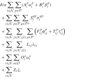
variable is set to 1. For continuous variables, it is a unit cost. The decision variables and the costs are presented in Table1. The mathematical model is as follows. The objective func-tion (1) minimizes procurement, producfunc-tion and transporta-tion fixed and variable costs.
Mi n i∈N p∈P (Aipαip+Bipβip) + i∈N p∈P q∈Pp Siq pσiq p + i∈N j∈N\{i} p∈P Fi jpφi jp+Ti jpτi jp + i∈N j∈N\{i} Li jλi j + i∈N o∈O Oioωio + i∈N Ziζi (1)
Constraints (2) to (6) are flow constraints. The sources are the component flows from the suppliers to the production centers, the sinks are the final product flows to customers. Constraint (2) considers the flow of each product assembly manufactured at each production center.
Aip+ j∈U\{i} Fj ip+ q∈Pp Siq p = j∈U\{i} Fi jp+ q∈M∪F gq pAqi + q/p∈Pq Sipq ∀i ∈U, ∀p ∈M (2)
Constraint (3) considers the flow of each component at each production center.
j∈(S∪U)\{i} Fj ip+ q∈Pp Siq p = j∈U\{i} Fi jp+ q∈M∪F gq pAqi + q/p∈Pq Sipq ∀i ∈U, ∀p ∈R (3)
Constraint (4) considers the flow of each component from each supplier.
Aip=
j∈U
Fi jp ∀i ∈S, ∀p∈R (4)
Constraint (5) considers the flow of each final product to each distribution center.
j∈U∪D\{i}
Fj ip =
j∈D∪C\{i}
Constraint (6) considers the flow of each final product from each production center.
Aip+
j∈U
Fj ip=
j∈D∪C\{i}
Fi jp ∀i ∈U, ∀p∈F (6) Constraint (7) ensures the customer’s demands have been satisfied. j∈D Fi jp+ q∈Pp Siq p = q/p∈Pq Sipq+dip ∀i ∈C,∀p∈F (7) Constraint (8) ensures that Bipis set to 1 if a production of p occurs. It also ensures that fixed costs are paid when a component is provided by a supplier or when an assem-bly is manufactured at a center. Amaxp is the upper bound of
Aip ∀i ∈U .
Aip≤BipAmaxp ∀i∈S∪U∪D,∀p∈P (8) Constraint (9) ensures that Zi is set to 1 if production center i is used.
Bip≤ Zi ∀i ∈S∪U∪D,∀p∈P (9) Constraint (10) defines the capacity of each technology needed at a center. p/u∈Pp lptAip≤ o∈Ot Oioco ∀i∈U,∀t ∈T (10)
Constraint (11) ensures that Ti jpis set to 1 if the arc from
i to j is used by at least one product p. Amaxp is the upper bound of Ti jp.
Fi jp≤Ti jpAmaxp ∀i ∈N,∀j ∈N\{i},∀p∈P (11) Constraint (12) ensures that Li j is set to 1 if at least one product uses the arc from i to j .
Ti jp≤Li j ∀i ∈N,∀j ∈N\{i},∀p∈P (12) Constraint (13) limits the number of substituted prod-ucts to be used at the production center in which they were created. q∈Pp Siq p ≤ q∈M\p gq pAqi + j∈C Fi jp ∀i ∈U,∀p∈P (13)
Robust design methodology
From the definitions of robustness presented in “Robustness assessment in supply chain design” section, we consider as robust a supply chain network design that can adapt to all plausible future scenarios—in this paper, a scenario is a set of parameters corresponding on normal conditions as well as major disruptions—by providing a solution that is close to optimal for each scenario (the proximity concept will be defined at the end of this section). In order to find a robust design, a methodology in three steps is followed, as shown in Fig.1.
In the first step, possible scenarios are generated and their optimal designs calculated. In the second step, the robustness of each design is assessed for each scenario. In the final step, a decision is made on the most robust design.
Step 1. Scenario generation The methodology proposed here is based on the generation of scenarios that reflect the parameters of the problem. All the uncer-tain parameters (e.g. demands, transportation costs, labor rates, …) are tested within a range of levels, depending on the probability of occurrence of each scenario and its impact on the solution. When the number of variables and levels is not too high, a fac-torial combination can be computed to generate the scenarios. Each scenario has a probability of occur-rence equal to the product of multiplying the indi-vidual probability levels. When the combinatorial explosion is too high, the number of levels has to be reduced for variables that don’t have a strong impact on the solution. Two methods can be used to assess the influence of a variable on the output: design of experiment (Taguchi 1986) and data mining (Dani 2009). A variable with a major influence should be tested precisely. We do not address this problem in depth here.
Then, the optimal design (design(l) in Fig.1) is com-puted for each scenario to determine the investments it needs and its objective value (obj(l) in Fig. 1) for each scenario (i). The investment in the opti-mal design in Step 2 refers to miniopti-mal investment constraints, and the objective value is the base on which to assess the robustness of the design for each scenario.
In Fig.1, scenario generation is based on the varia-tion of two parameters on two levels Four scenarios are generated and solved.
Step 2. Robustness assessment Here, the robustness of each design applied to each scenario is evaluated. Choosing a design involves some investments. We consider that once a design is chosen, investments are made. When the real scenario is known, the
Fig. 1 Robust design
methodology
supply chain can change, but there will be some investments that have already been made (e.g. at pro-duction centers and in terms of equipment acquisi-tion). So, we proceed with a new optimization to determine the most efficient supply chain, taking into account the investment that has already been made, as some decision variables were fixed in Step 1 (e.g. nodes opened, production lines organized and specific equipment bought, and transportation arranged). In this step, each scenario is solved again for each design created in Step 1, including the extra constraints that correspond to the investments made in each design (Cont (l) in Fig.1). Constraint (14) applies to production centers, (15) to production line investments, (16) to specific equipment and (17) to arranging transportation.
Zi ≥Solk(Zi) ∀i ∈U (14)
Bip≥Solk(Bip) ∀i ∈S∪U∪D,∀p∈P (15)
Oio≥Solk(Oio) ∀i ∈U,∀o∈O (16)
Li j ≥Solk(Li j) ∀i ∈N,∀j ∈N \ {i}, (17)
The objective value generated in Step 2 is then com-pared to the optimal solution of the original scenario (obj(l)). The robustness of a solution k on a scenario
l is assessed by formula (18), which represents the gap between the objective value of the optimal solu-tion when considering scenario k and the optimal solution.
r obust nessk(l)=
objk(l)−obj(l)
obj(l) (18)
A value of 0 means perfect robustness, and the higher the value, the less robust the solution. Note that r obustnessk(k)=0 and r obustnessk(l)≥0, i.e. the solution is optimal if the effective scenario is the one that has been scheduled, otherwise it is worse.
Step 3. Design selection A design has to be chosen from all the scenarios generated based on their robustness in all of them.
Several criteria can be used to classify the designs:
Table 2 Results example to illustrate Steps 2 and 3
Prob. Design 1 Design 2 Design 3 Design 4
Scenario 1 0.20 0.00 0.90 0.90 10.00 Scenario 2 0.30 0.50 0.00 0.80 0.10 Scenario 3 0.10 1.50 1.00 0.00 0.20 Scenario 4 0.40 0.20 0.25 0.60 0.00 Minmax 1.50 1.00 0.90 10.00 Average robustness 0.38 0.38 0.66 2.05 Minumum standard deviation 0.41 0.38 0.25 3.98 Least beyond the threshold (20 %) 2 3 3 1
Best values are given in bold
Productioncenters Distributioncenters Suppliers Customers
Fig. 2 Geographical position of the potential nodes in the case study
• Minmax: a design that minimizes the possible loss for a worst-case scenario.
• Average robustness: a design that is close, on average, to the optimal solution for each scenario.
• Minimum standard deviation: a design that is more sta-ble than the others for each scenario. It can be used to differentiate between two designs with the same minmax or the same average robustness.
• Least beyond the threshold: a design that limits unaccept-able solutions. This threshold has to be fixed.
Depending on the acceptable risk, the decision favors designs in the minmax and minimum standard deviation categories, in order to avoid the worst-case scenarios, and designs in the average robustness category for the best expected value.
Table2illustrates Steps 2 and 3 of the methodology with four scenarios.
Once Step 1 has been completed, four scenarios will have been generated, each with a probability of occurrence (20 % for scenario 1, 30 % for scenario 2 and so on…). The model is optimized for each of these scenarios, and yields four designs. To assess the robustness of these designs, Step 2 is applied, giving the robustness of each design on each scenario. Step 3 aggregates the results and assesses each design. Design 1 has the best average robustness (38 %); however, its standard deviation is high (41 %), its maximum possible loss is 150 %, and two scenarios are beyond the threshold, which was set at 20 %. Design 2 has similar results, but with a better max-imum loss (100 %) and standard deviation (38 %), and more results beyond the threshold. Design 3 is the least risky, as it has the lowest maximum loss and the minimum standard deviation, but its expected value is above that of Designs 1 and 2. Design 4 has poor results because of its maximum loss of 1,000 %, caused by scenario 1 while the other scenarios are well predicted, and so this is the best design with respect to the threshold criterion.
The complexity of the algorithm isO(n2), with n being the number of scenarios. This means that a reasonable num-ber of scenarios has to be considered, as the resolution of a single problem is not negligible. For example,Baud-Lavigne et al.(2011) experiment with a resolution time of around 1 second for cases with 10 production centers and 20 parts, 5 min for 10 production centers and 100 parts, and 30 min for 15 production centers and 150 parts.
Experiments to illustrate the methodology
Experiments were conducted involving solution of the MILP presented in “The design” section with ILOG CPLEX 12.5 Java libraries on a laptop with a Intel Core2Duo CPU at 2.26 GHz and 4 GB RAM.
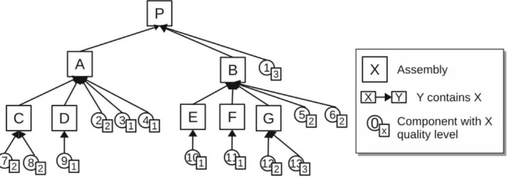
Fig. 3 Root BOM for the
Fig. 4 Bill of materials for three products
Table 3 Cost characteristics of the case study
Fixed costs Value
Per (axe, product) $200
Per (component, supplier) $1,000
Per (product, production center) $50,000
Per supplier $5,000
Per production center $200,000
Per DC $10,000
Table 4 Uncertain parameters in the case study
Parameter Tested values Logistical costs 50/100/150$/m3
Labor costs Units 1, 2: 15/20/25—units 3, 4: 5/10/15 $/h
Demand 50/100/150 %
The case study was taken from the generator proposed inBaud-Lavigne et al.(2011), with two markets areas, four production centers (two per market), and two distribution
Table 5 Results of the Pareto-optimal solutions
Prob. Design 4 (%) Design 7 (%)
Minmax 1.8 1.1
Average robustness 0.1 0.4
Minimum standard deviation 0.3 0.2
Least beyond the threshold (1 %) 1.2 2.5 Best values are given in bold
centers (Fig.2); a family of nine products with a three level BOM. Each product is an instance of the root BOM presented in Fig.3, with 8 assemblies and 13 components. Each com-ponent can be present or not and has different quality level possibilities. These combinations define products sold by the company. Figure4illustrates three products P1, P2and P3,
of the nine in the product family. The size of the problem is small, in order to speed up the experiment.
Table3shows the parameters used in this case study. Step 1. Scenario generation Scenarios are generated from
variation of the following parameters as described
sol1 sol2 sol3 sol4 sol5 sol6 sol7 sol8 sol9 sol10 sol11 sol12 sol13 sol14 sol15 sol16 sol17 sol18 sol19 sol20 sol21 sol22 sol23 sol24 sol25 sol26 sol27 sol28 sol29 sol30 sol31 sol32 sol33 sol34 sol35 sol36 sol37 sol38 sol39 sol40 sol41 sol42 sol43 sol44 sol45 sol46 sol47 sol48 sol49 sol50 sol51 sol52 sol53 sol54 sol55 sol56 sol57 sol58 sol59 sol60 sol61 sol62 sol63 sol64 sol65 sol66 sol67 sol68 sol69 sol70 sol71 sol72 sol73 sol74 sol75 sol76 sol77 sol78 sol79 sol80 sol81 0 0.01 0.02 0.03 0.04 0.05 0.06 0 0.05 0.1 0.15 0.2 0.25 0.3 0.35 0.4 0.45
max avg std dev Threshold
Production centers Distribution centers Suppliers Customers
Fig. 6 Relative geographical location of the supply chain components
in Design 4
in Table4: demand (3 levels), transportation costs (3 levels), and labor costs (3 levels in two units). These parameters and their levels are determined to illustrate our method. In an industrial case study, a systematic methodology should be used to determine these scenarios, as seen in “Robust design method-ology” section. This leads to 81 scenarios, resulting from the combination of each level and each para-meter. Then, each scenario is solved, resulting in 81 designs.
Step 2. Robustness assessment The robustness of the 81 designs is assessed by determining their robustness relative to that of each of the 81 scenarios constrained by these designs.
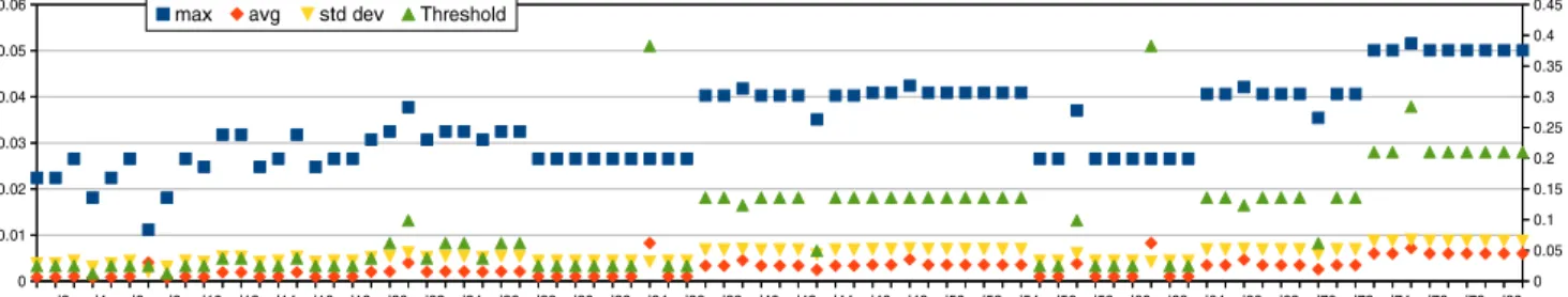
Step 3. Design selection Results for all the designs are illus-trated in Fig.5.
For each design on the X-axis, the robustness results for all the scenarios are aggregated on the four crite-ria, following Step 3 of the methodology: measuring maximal loss, average loss, standard deviation (left Y-axis) and threshold (right Y-axis). Results of the Pareto optimal solutions, Design(4) and Design(7), are presented in Table5. The supply chain of the two designs is identical and is presented in Fig.6.
Fig. 8 Actual bill of materials of product P3in Design 7
The actual bill of materials of the two designs are presented in Figs.7and8. They are identical at the following points: Product P1is produced as-is and is
used instead of 5 others products (P5to P9); product
P2is close to the original one, only component 6.1
has been standardized by component 6.2; it defers for product 3, as Design (4) standardizes B2 by B1 contained in P1, and Design (7) standardizes B2 by
B4 contained in P4 (not illustrated here).
Based on the minmax criterion, Design 7 would be chosen, because its maximum loss value is the lowest of all the designs. Nevertheless, it has a high average robustness value, but a low standard deviation. This means that Design 7 is a reliable solution, which can adapt to all possible scenarios, but falls short of the optimal solution. By contrast, Design 4 has a very low average robustness value, but its standard deviation is a bit higher than that of Design 7 and its worst result is nearly twice as high.
Conclusion
This paper has addressed the problem of robustness in the joint product family and supply chain design problem.
The proposed methodology allows us to find a design that best suits all the possible parameter variations. Depending on
the risk the company is able to take, several decision plans are proposed, based on four indicators. Its aim is to choose the design that is either the most profitable or the most reliable, or a good balance of the two.
The optimization method proposed in this paper can be used to explore a wide range of designs with little configu-ration required. However, the computation time is high, in the range of the square of the number of solutions explored. There are two possible ways to shorten this time. The first is to reduce the number of scenarios by changing the way they are generated. The design of experiment or data mining methods could be an important step in doing so. The second is to cre-ate designs that are not based on scenario optimization. If we know that none of the predicted scenarios will occur, newer, better fitting designs can be created from several scenarios using genetic algorithm.
References
Baud-Lavigne, B., Agard, B., & Penz, B. (2011). A MILP model for joint product family and supply chain design. In Proceedings of the International Conference on Industrial Engineering and Systems Management (IESM’2011), Metz, France (pp. 889–897). Interna-tional Institute for Innovation, Industrial Engineering and Entrepre-neurship (I4e2). ISBN 978-2-9600532-3-4.
Baud-Lavigne, B., Agard, B., & Penz, B. (2012). Mutual impacts of product standardization and supply chain design. International Jour-nal of Production Economics, 135(1), 50–60.
Chan, F. T. S., Chung, S. H., & Choy, K. L. (2006). Optimization of order fulfillment in distribution network problems. Journal of Intelligent Manufacturing, 17(3), 307–319.
Chen, H.-Y. (2010). The impact of item substitutions on production– distribution networks for supply chains. Transportation Research Part E: Logistics and Transportation Review, 46(6), 803–819. Childerhouse, P., & Towill, D. R. (2004). Reducing uncertainty in
Euro-pean supply chains. Journal of Manufacturing Technology Manage-ment, 15(7), 585–598.
Dani, S. (2009). Predicting and managing supply chain risks. In Supply Chain, Risk (pp. 53–66). Berlin: Springer.
El Hadj Khalaf, R., Agard, B., & Penz, B. (2010). An experimental study for the selection of modules and facilities in a mass customization context. Journal of Intelligent Manufacturing, 21(6), 703–716. ElMaraghy, H., & Mahmoudi, N. (2009). Concurrent design of product
modules structure and global supply chain configurations. Interna-tional Journal of Computer Integrated Manufacturing, 22(6), 483– 493.
Jiao, J., Simpson, T., & Siddique, Z. (2007). Product family design and platform-based product development: A state-of-the-art review. Journal of Intelligent Manufacturing, 18(1), 5–29.
Klibi, W., Martel, A., & Guitouni, A. (2010). The design of robust value-creating supply chain networks: A critical review. European Journal of Operational Research, 203(2), 283–293.
Kristianto, Y., Helo, P., & Jiao, R. (2013). Mass customization design of engineer-to-order products using benders’ decomposition and bi-level stochastic programming. Journal of Intelligent Manufacturing, 24(5), 961–975.
Lamothe, J., Hadj-Hamou, K., & Aldanondo, M. (2006). An optimiza-tion model for selecting a product family and designing its supply chain. European Journal of Operational Research, 169(3), 1030– 1047.
Meepetchdee, Y., & Shah, N. (2007). Logistical network design with robustness and complexity considerations. International Journal of Physical Distribution and Logistics Management, 37(3), 201–222. Mohammadi Bidhandi, H., & Mohd Yusuff, R. (2011). Integrated
sup-ply chain planning under uncertainty using an improved stochastic approach. Applied Mathematical Modelling, 35(6), 2618–2630. Pan, F., & Nagi, R. (2010). Robust supply chain design under
uncer-tain demand in agile manufacturing. Computers and Operations Research, 37(4), 668–683.
Parvaresh, F., Husseini, S. M. M., Golpayegany, S. A. H., & Karimi, B. (2012). Hub network design problem in the presence of dis-ruptions. Journal of Intelligent Manufacturing, 1–20. doi:10.1007/ s10845-012-0717-7.
Peidro, D., Mula, J., Poler, R., & Lario, F. (2009). Quantitative models for supply chain planning under uncertainty: A review. The Interna-tional Journal of Advanced Manufacturing Technology, 43(3), 400– 420.
Schulze, L., & Li, L. (2009). Location-allocation model for logistics networks with implementing commonality and postponement strate-gies. Proceedings of the International MultiConference of Engineers and Computer Scientists, 2, 1615–1620.
Shahzad, K. M., & Hadj-Hamou, K. (2013). Integrated supply chain and product family architecture under highly customized demand. Journal of Intelligent Manufacturing, 24(5), 1005–1018.
Shapiro, J. F. (2001). Modeling the Supply Chain. Boston: Duxbury Resource Center.
Shimizu, Y., Fushimi, H., & Wada, T. (2011). Robust logistics network modeling and design against uncertainties. Journal of Advanced Mechanical Design, Systems, and Manufacturing, 5(2), 103–114. Taguchi, G. (1986). Introduction to quality engineering: Designing
quality into products and processes. Asian Productivity Organiza-tion.
Wie, M. V., Stone, R. B., Thevenot, H., & Simpson, T. (2007). Exam-ination of platform and differentiating elements in product family design. Journal of Intelligent Manufacturing, 18(1), 77–96. Zhang, X., Huang, G., Humphreys, P., & Botta-Genoulaz, V. (2010).
Simultaneous configuration of platform products and manufacturing supply chains: Comparative investigation into impacts of different supply chain coordination schemes. Production Planning and Con-trol, 21(6), 609.