Robust small area estimation

(1)

Dissertations

2008

Robust small area estimation

Lixia Diao

Iowa State University

Follow this and additional works at:

https://lib.dr.iastate.edu/rtd

Part of the

Statistics and Probability Commons

This Dissertation is brought to you for free and open access by the Iowa State University Capstones, Theses and Dissertations at Iowa State University Digital Repository. It has been accepted for inclusion in Retrospective Theses and Dissertations by an authorized administrator of Iowa State University Digital Repository. For more information, please [email protected].

Recommended Citation

Diao, Lixia, "Robust small area estimation" (2008).Retrospective Theses and Dissertations. 15809.

(2)

by

Lixia Diao

A dissertation submitted to the graduate faculty in partial fulfillment of the requirements for the degree of

DOCTOR OF PHILOSOPHY

Major: Statistics

Program of Study Committee: Jean D. Opsomer, Co-major Professor

Taps Maiti, Co-major Professor Gary Phye

Huaiqing Wu Cindy L. Yu

Iowa State University Ames, Iowa

2008

(3)

3316164

(4)

TABLE OF CONTENTS

LIST OF TABLES . . . iv

CHAPTER 1. Robust Small Area Estimation for the Fay-Herriot Model . 1 1.1 Introduction . . . 1

1.2 The FH Model and Small Area Estimation . . . 3

1.2.1 Model Parameter Estimation . . . 4

1.2.2 Finite Sample Performance . . . 8

1.3 Mean Squared Prediction Error of EBLUP . . . 11

1.4 Estimation of Mean Squared Prediction Error . . . 13

1.4.1 Mean Squared Prediction Error Estimation . . . 13

1.5 Conclusion . . . 18

CHAPTER 2. Accurate Confidence Interval Estimation of Small Area Pa-rameters under the Fay-Herriot Model . . . 19

2.1 Introduction . . . 19

2.2 The FH Model and Small Area Estimation . . . 21

2.3 Confidence Interval with Corrected Coverage Probability . . . 24

2.3.1 Confidence Interval with Corrected Coverage Probability . . . 24

2.4 Confidence Interval for the Difference of Two Small Areas . . . 32

2.4.1 Confidence Interval for the Difference of Two Small Areas . . . 32

(5)

CHAPTER 3. Model Assisted Design Consistent Small Area Estimator for

the Nested-Error Regression Model . . . 38

3.1 Introduction . . . 38

3.2 The Nested-Error Regression Model . . . 39

3.2.1 Model Parameter Estimation . . . 40

3.3 Small Area Estimation . . . 48

3.3.1 Small Area Mean Estimator . . . 48

3.4 Conclusion . . . 52

APPENDIX A. Theorems Proof for Chapter 1 . . . 54

APPENDIX B. Finite Sample Performance for Chapter 1 . . . 88

APPENDIX C. Theorem Proof for Chapter 2 . . . 133

APPENDIX D. Theorem Proof for Chapter 3 . . . 139

APPENDIX E. Finite Sample Performance for Chapter 3 . . . 151

(6)

LIST OF TABLES

Table 1.1 Coverage probabilities for nominal 95% confidence intervals using asymp-totic normality and estimated variances for four different estimators: Robust Estimation (RE), Fay-Herriot estimation, MME estimation, REML estimation, when both ui and εi are normal or centered chi-square distribution for Di in pattern(a). . . 10

Table 1.2 Bias and MSPE ofθib, Relative Bias and Relative Variability of mspe(θib)

for Robust Estimation (RE), Fay-Herriot estimation when bothui and

εi are Chi-squared distribution and D is pattern (a). . . 17

Table 2.1 Coverage probabilities (CP) and coverage length (CL) for nominal 95% confidence intervals for pattern (a). The first number in each cell is the result for our proposed method and the second one (in parentheses) is the naive FH method. . . 29 Table 2.2 Coverage probabilities (CP) and coverage length (CL) for nominal 95%

confidence intervals for pattern (b). The first number in each cell is the result for our proposed method and the second one (in parentheses) is the naive FH method. . . 30 Table 2.3 Coverage probabilities (CP) and coverage length (CL) for nominal 95%

confidence intervals for pattern (c). The first number in each cell is the result for our proposed method and the second one (in parentheses) is the naive FH method. . . 31

(7)

Table 2.4 Coverage probabilities (CP) and coverage length (CL) for nominal 95% confidence intervals for the proposed method for the scenarios consid-ered in Chatterjeeet al. (2007). . . 31 Table 2.5 Coverage probabilities (CP) and coverage length (CL) for nominal 95%

confidence intervals the difference between two small area means for pattern (a). The first number in each cell is the result for our proposed method and the second one (in parentheses) is the naive FH method. . 34 Table 2.6 Coverage probabilities (CP) and coverage length (CL) for nominal 95%

confidence intervals the difference between two small area means for pattern (b). The first number in each cell is the result for our proposed method and the second one (in parentheses) is the naive FH method. . 35 Table 2.7 Coverage probabilities (CP) and coverage length (CL) for nominal 95%

confidence intervals the difference between two small area means for pattern (c). The first number in each cell is the result for our proposed method and the second one (in parentheses) is the naive FH method. . 36

Table 3.1 Bias, root mean square error for β, σ2

u and σe2 for Robust Estimation

(RE) across different scenarios determined by the variance ratioR. . . 46 Table 3.2 Bias, root mean square error for β, σ_u2 and σ_e2 for Fuller’s estimation

across different scenarios determined by the variance ratioR. . . 47 Table 3.3 Variance for θb_gR, θb_gF and θb_{gF p} over all areas comparing to population

estimator θgpop across different scenarios determined by the variance ratioR. . . 51 Table 3.4 Bias, variance and root mean square error forθgRb ,θgFb andθgF pb over all

areas comparing to population estimatorθgpop across different scenarios determined by the variance ratioR. . . 51 Table 3.5 Bias, variance and root mean square error for θgRb , θgFb and θgF pb over

all areas comparing to true mean of areaθgT across different scenarios

(8)

Table 3.6 Bias and root mean square error for θb_gR, θb_gF and θb_{gF p} over all areas

comparing to area meanθgacross different scenarios determined by the variance ratioR. . . 52

Table B.1 Bias, mean square error for β and σ2_u, estimated standard deviation, coverage probabilities and coverage length of nominal 95% confidence intervals forσ_u2 using asymptotic normality and estimated variances for Robust Estimation (RE) when both ui and εi are normal distribution and D in pattern (a). . . 88 Table B.2 Bias, mean square error for β and σ2_u, estimated standard deviation,

coverage probabilities and coverage length of nominal 95% confidence intervals forσ_u2 using asymptotic normality and estimated variances for Fay-Herriot estimation when bothuiandεiare normal distribution and D in pattern (a). . . 89 Table B.3 Bias, mean square error for β and σ2_u, estimated standard deviation,

coverage probabilities and coverage length of nominal 95% confidence intervals forσ2

u using asymptotic normality and estimated variances for

MME estimation when bothui andεi are normal distribution and D in

pattern (a). . . 89 Table B.4 Bias, mean square error for β and σ2_u, estimated standard deviation,

coverage probabilities and coverage length of nominal 95% confidence intervals forσ_u2 using asymptotic normality and estimated variances for REML estimation when bothui and εi are normal distribution and D

in pattern (a). . . 90 Table B.5 Bias, mean square error for β and σ2_u, estimated standard deviation,

coverage probabilities and coverage length of nominal 95% confidence intervals forσ_u2 using asymptotic normality and estimated variances for Robust Estimation (RE) when ui is centered chi-square distribution

(9)

Table B.6 Bias, mean square error for β and σ2_u, estimated standard deviation, coverage probabilities and coverage length of nominal 95% confidence intervals forσ_u2 using asymptotic normality and estimated variances for Fay-Herriot estimation when ui is centered chi-square distribution and

εi is normal distribution and D in pattern (a). . . 91 Table B.7 Bias, mean square error for β and σ2_u, estimated standard deviation,

MME estimation when ui is centered chi-square distribution and εi is

normal distribution and D in pattern (a). . . 91 Table B.8 Bias, mean square error for β and σ2_u, estimated standard deviation,

coverage probabilities and coverage length of nominal 95% confidence intervals forσ_u2 using asymptotic normality and estimated variances for REML estimation whenui is centered chi-square distribution and εi is

normal distribution and D in pattern (a). . . 92 Table B.9 Bias, mean square error for β and σ2_u, estimated standard deviation,

coverage probabilities and coverage length of nominal 95% confidence intervals forσ_u2 using asymptotic normality and estimated variances for Robust Estimation (RE) when both ui and εi are centered chi-square

distribution and D in pattern (a). . . 92 Table B.10 Bias, mean square error for β and σ2_u, estimated standard deviation,

coverage probabilities and coverage length of nominal 95% confidence intervals for σ_u2 using asymptotic normality and estimated variances for Fay-Herriot estimation when bothui andεi are centered chi-square distribution and D in pattern (a). . . 93

(10)

Table B.11 Bias, mean square error for β and σ2_u, estimated standard deviation, coverage probabilities and coverage length of nominal 95% confidence intervals forσ_u2 using asymptotic normality and estimated variances for MME estimation when bothui andεi are centered chi-square distribu-tion and D in pattern (a). . . 93 Table B.12 Bias, mean square error for β and σ2_u, estimated standard deviation,

REML estimation when both ui and εi are centered chi-square

distri-bution and D in pattern (a). . . 94 Table B.13 Bias, mean square error for β and σ2_u, estimated standard deviation,

coverage probabilities and coverage length of nominal 95% confidence intervals for σ_u2 using asymptotic normality and estimated variances for Robust Estimation (RE) whenui is t distribution and εi is normal

coverage probabilities and coverage length of nominal 95% confidence intervals for σ_u2 using asymptotic normality and estimated variances for Fay-Herriot estimation when ui is t distribution and εi is normal

coverage probabilities and coverage length of nominal 95% confidence intervals forσ_u2 using asymptotic normality and estimated variances for MME estimation whenui is t distribution andεiis normal distribution and D in pattern (a). . . 96

(11)

Table B.16 Bias, mean square error for β and σ2_u, estimated standard deviation, coverage probabilities and coverage length of nominal 95% confidence intervals forσ_u2 using asymptotic normality and estimated variances for REML estimation whenuiis t distribution andεiis normal distribution and D in pattern (a). . . 96 Table B.17 Bias, mean square error for β and σ2_u, estimated standard deviation,

Robust Estimation (RE) when ui and εi are t distribution and D in

coverage probabilities and coverage length of nominal 95% confidence intervals for σ_u2 using asymptotic normality and estimated variances for Fay-Herriot estimation when ui and εi are t distribution and D in

coverage probabilities and coverage length of nominal 95% confidence intervals forσ_u2 using asymptotic normality and estimated variances for MME estimation whenui and εi are t distribution and D in pattern (a). 98

Table B.20 Bias, mean square error for β and σ2_u, estimated standard deviation, coverage probabilities and coverage length of nominal 95% confidence intervals forσ_u2 using asymptotic normality and estimated variances for REML estimation whenui and εi are t distribution and D in pattern (a). 99 Table B.21 Bias, mean square error for β and σ2_u, estimated standard deviation,

coverage probabilities and coverage length of nominal 95% confidence intervals forσ_u2 using asymptotic normality and estimated variances for Robust Estimation (RE) whenui andεi are normal distribution and D in pattern (b). . . 99

(12)

Table B.22 Bias, mean square error for β and σ2_u, estimated standard deviation, coverage probabilities and coverage length of nominal 95% confidence intervals forσ_u2 using asymptotic normality and estimated variances for Fay-Herriot estimation when ui and εi are normal distribution and D in pattern (b). . . 100 Table B.23 Bias, mean square error for β and σ2_u, estimated standard deviation,

coverage probabilities and coverage length of nominal 95% confidence intervals for σ2

u using asymptotic normality and estimated variances

for MME estimation when ui and εi are normal distribution and D in

pattern (b). . . 100 Table B.24 Bias, mean square error for β and σ2_u, estimated standard deviation,

coverage probabilities and coverage length of nominal 95% confidence intervals forσ_u2 using asymptotic normality and estimated variances for REML estimation when ui and εi are normal distribution and D in

coverage probabilities and coverage length of nominal 95% confidence intervals forσ_u2 using asymptotic normality and estimated variances for Robust Estimation (RE) when ui is centered chi-squared distribution

and εi is normal distribution and D in pattern (b). . . 101

Table B.26 Bias, mean square error for β and σ2_u, estimated standard deviation, coverage probabilities and coverage length of nominal 95% confidence intervals forσ_u2 using asymptotic normality and estimated variances for Fay-Herriot estimation whenuiis centered chi-squared distribution and

(13)

Table B.27 Bias, mean square error for β and σ2_u, estimated standard deviation, coverage probabilities and coverage length of nominal 95% confidence intervals forσ_u2 using asymptotic normality and estimated variances for MME estimation whenui is centered chi-squared distribution andεi is normal distribution and D in pattern (b). . . 102 Table B.28 Bias, mean square error for β and σ2_u, estimated standard deviation,

REML estimation when ui is centered chi-squared distribution and εi

is normal distribution and D in pattern (b). . . 103 Table B.29 Bias, mean square error for β and σ2_u, estimated standard deviation,

coverage probabilities and coverage length of nominal 95% confidence intervals for σ_u2 using asymptotic normality and estimated variances for Robust Estimation (RE) when ui and εi are centered chi-squared

distribution and D in pattern (b). . . 103 Table B.30 Bias, mean square error for β and σ2_u, estimated standard deviation,

coverage probabilities and coverage length of nominal 95% confidence intervals forσ_u2 using asymptotic normality and estimated variances for Fay-Herriot estimation whenui and εi are centered chi-squared

distri-bution and D in pattern (b). . . 104 Table B.31 Bias, mean square error for β and σ2_u, estimated standard deviation,

coverage probabilities and coverage length of nominal 95% confidence intervals forσ_u2 using asymptotic normality and estimated variances for MME estimation whenui and εi are centered chi-squared distribution and D in pattern (b). . . 104

(14)

Table B.32 Bias, mean square error for β and σ2_u, estimated standard deviation, coverage probabilities and coverage length of nominal 95% confidence intervals forσ_u2 using asymptotic normality and estimated variances for REML estimation whenui andεi are centered chi-squared distribution and D in pattern (b). . . 105 Table B.33 Bias, mean square error for β and σ2_u, estimated standard deviation,

for Robust Estimation (RE) whenui is t distribution and εi is normal

coverage probabilities and coverage length of nominal 95% confidence intervals for σ_u2 using asymptotic normality and estimated variances for Fay-Herriot estimation when ui is t distribution and εi is normal

coverage probabilities and coverage length of nominal 95% confidence intervals forσ_u2 using asymptotic normality and estimated variances for MME estimation whenui is t distribution andεiis normal distribution

and D in pattern (b). . . 107 Table B.36 Bias, mean square error for β and σ2_u, estimated standard deviation,

coverage probabilities and coverage length of nominal 95% confidence intervals forσ_u2 using asymptotic normality and estimated variances for REML estimation whenuiis t distribution andεiis normal distribution and D in pattern (b). . . 107

(15)

Table B.37 Bias, mean square error for β and σ2_u, estimated standard deviation, coverage probabilities and coverage length of nominal 95% confidence intervals forσ_u2 using asymptotic normality and estimated variances for Robust Estimation (RE) when ui and εi are t distribution and D in pattern (b). . . 108 Table B.38 Bias, mean square error for β and σ2_u, estimated standard deviation,

for Fay-Herriot estimation when ui and εi are t distribution and D in

coverage probabilities and coverage length of nominal 95% confidence intervals forσ_u2 using asymptotic normality and estimated variances for MME estimation whenui and εi are t distribution and D in pattern (b).109

Table B.40 Bias, mean square error for β and σ2_u, estimated standard deviation, coverage probabilities and coverage length of nominal 95% confidence intervals forσ_u2 using asymptotic normality and estimated variances for REML estimation whenui andεi are t distribution and D in pattern (b).109 Table B.41 Bias, mean square error for β and σ2

u, estimated standard deviation,

coverage probabilities and coverage length of nominal 95% confidence intervals forσ_u2 using asymptotic normality and estimated variances for Robust Estimation (RE) whenui andεi are normal distribution and D

in pattern (c). . . 110 Table B.42 Bias, mean square error for β and σ2_u, estimated standard deviation,

coverage probabilities and coverage length of nominal 95% confidence intervals forσ_u2 using asymptotic normality and estimated variances for Fay-Herriot estimation when ui and εi are normal distribution and D in pattern (c). . . 110

(16)

Table B.43 Bias, mean square error for β and σ2_u, estimated standard deviation, coverage probabilities and coverage length of nominal 95% confidence intervals for σ_u2 using asymptotic normality and estimated variances for MME estimation when ui and εi are normal distribution and D in pattern (c). . . 111 Table B.44 Bias, mean square error for β and σ2_u, estimated standard deviation,

REML estimation when ui and εi are normal distribution and D in

pattern (c). . . 111 Table B.45 Bias, mean square error for β and σ2_u, estimated standard deviation,

coverage probabilities and coverage length of nominal 95% confidence intervals forσ_u2 using asymptotic normality and estimated variances for Robust Estimation (RE) when ui is centered chi-square distribution

and εi is normal distribution and D in pattern (c). . . 112 Table B.46 Bias, mean square error for β and σ2_u, estimated standard deviation,

coverage probabilities and coverage length of nominal 95% confidence intervals forσ_u2 using asymptotic normality and estimated variances for Fay-Herriot estimation when ui is centered chi-square distribution and εi is normal distribution and D in pattern (c). . . 112

Table B.47 Bias, mean square error for β and σ2_u, estimated standard deviation, coverage probabilities and coverage length of nominal 95% confidence intervals forσ_u2 using asymptotic normality and estimated variances for MME estimation when ui is centered chi-square distribution and εi is normal distribution and D in pattern (c). . . 113

(17)

Table B.48 Bias, mean square error for β and σ2_u, estimated standard deviation, coverage probabilities and coverage length of nominal 95% confidence intervals forσ_u2 using asymptotic normality and estimated variances for REML estimation whenui is centered chi-square distribution and εi is normal distribution and D in pattern (c). . . 113 Table B.49 Bias, mean square error for β and σ2_u, estimated standard deviation,

for Robust Estimation (RE) when ui and εi are centered chi-square

distribution and D in pattern (c). . . 114 Table B.50 Bias, mean square error for β and σ2_u, estimated standard deviation,

coverage probabilities and coverage length of nominal 95% confidence intervals forσ_u2 using asymptotic normality and estimated variances for Fay-Herriot estimation whenui andεi are centered chi-square

distribu-tion and D in pattern (c). . . 114 Table B.51 Bias, mean square error for β and σ2_u, estimated standard deviation,

coverage probabilities and coverage length of nominal 95% confidence intervals forσ_u2 using asymptotic normality and estimated variances for MME estimation when ui and εi are centered chi-square distribution

and D in pattern (c). . . 115 Table B.52 Bias, mean square error for β and σ2_u, estimated standard deviation,

coverage probabilities and coverage length of nominal 95% confidence intervals forσ_u2 using asymptotic normality and estimated variances for REML estimation when ui and εi are centered chi-square distribution and D in pattern (c). . . 116

(18)

Table B.53 Bias, mean square error for β and σ2_u, estimated standard deviation, coverage probabilities and coverage length of nominal 95% confidence intervals for σ_u2 using asymptotic normality and estimated variances for Robust Estimation (RE) whenui is t distribution and εi is normal distribution and D in pattern (c). . . 116 Table B.54 Bias, mean square error for β and σ2_u, estimated standard deviation,

for Fay-Herriot estimation when ui is t distribution and εi is normal

distribution and D in pattern (c). . . 117 Table B.55 Bias, mean square error for β and σ2_u, estimated standard deviation,

coverage probabilities and coverage length of nominal 95% confidence intervals forσ_u2 using asymptotic normality and estimated variances for MME estimation whenui is t distribution andεiis normal distribution

coverage probabilities and coverage length of nominal 95% confidence intervals forσ_u2 using asymptotic normality and estimated variances for REML estimation whenuiis t distribution andεiis normal distribution

coverage probabilities and coverage length of nominal 95% confidence intervals forσ_u2 using asymptotic normality and estimated variances for Robust Estimation (RE) when ui and εi are t distribution and D in pattern (c). . . 118

(19)

Table B.58 Bias, mean square error for β and σ2_u, estimated standard deviation, coverage probabilities and coverage length of nominal 95% confidence intervals for σ_u2 using asymptotic normality and estimated variances for Fay-Herriot estimation when ui and εi are t distribution and D in pattern (c). . . 119 Table B.59 Bias, mean square error for β and σ2_u, estimated standard deviation,

MME estimation whenui and εi are t distribution and D in pattern (c). 119

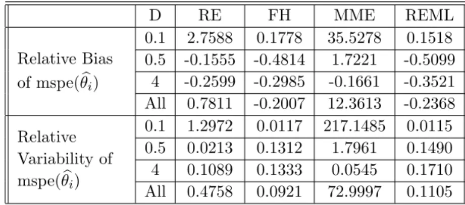
Table B.60 Bias, mean square error for β and σ2_u, estimated standard deviation, coverage probabilities and coverage length of nominal 95% confidence intervals forσ_u2 using asymptotic normality and estimated variances for REML estimation when both ui and εi are t distribution and D in in pattern (c). . . 120 B.61 Relative Bias,Relative Variability and Coverage Probability of mspe(θib)

for Robust Estimation (RE), Fay-Herriot estimation, MME estimation, REML estimation when both ui and εi are Chi-squared distribution,

n=15 and D is pattern (a). . . 120 Table B.62 Relative Bias,Relative Variability and Coverage Probability of mspe(θb_i)

for Robust Estimation (RE), Fay-Herriot estimation, MME estimation, REML estimation when both ui and εi are Chi-squared distribution, n=15 and D is pattern (b). . . 121 Table B.63 Relative Bias,Relative Variability and Coverage Probability of mspe(θib)

(20)

Table B.64 Relative Bias,Relative Variability and Coverage Probability of mspe(θib)

n=15 and D is pattern (d). . . 122 Table B.65 Relative Bias,Relative Variability and Coverage Probability of mspe(θib)

for Robust Estimation (RE), Fay-Herriot estimation, MME estimation, REML estimation when both ui and εi are Exponential distribution, n=15 and D is pattern (a). . . 122 Table B.66 Relative Bias,Relative Variability and Coverage Probability of mspe(θb_i)

for Robust Estimation (RE), Fay-Herriot estimation, MME estimation, REML estimation when both ui and εi are Exponential distribution,

n=15 and D is pattern (b). . . 123 Table B.67 Relative Bias,Relative Variability and Coverage Probability of mspe(θib)

for Robust Estimation (RE), Fay-Herriot estimation, MME estimation, REML estimation when both ui and εi are Exponential distribution, n=15 and D is pattern (c). . . 123 Table B.68 Relative Bias,Relative Variability and Coverage Probability of mspe(θb_i)

for Robust Estimation (RE), Fay-Herriot estimation, MME estimation, REML estimation when both ui and εi are Normal distribution, n=15 and D is pattern (a). . . 125 Table B.70 Relative Bias,Relative Variability and Coverage Probability of mspe(θb_i)

for Robust Estimation (RE), Fay-Herriot estimation, MME estimation, REML estimation when both ui and εi are Normal distribution, n=15 and D is pattern (b). . . 125

(21)

for Robust Estimation (RE), Fay-Herriot estimation, MME estimation, REML estimation when both ui and εi are Normal distribution, n=15

and D is pattern (c). . . 126 Table B.72 Relative Bias,Relative Variability and Coverage Probability of mspe(θib)

for Robust Estimation (RE), Fay-Herriot estimation, MME estimation, REML estimation when both ui and εi are Normal distribution, n=15 and D is pattern (d). . . 126 Table B.73 Relative Bias,Relative Variability and Coverage Probability of mspe(θb_i)

n=30 and D is pattern (a). . . 127 Table B.74 Relative Bias,Relative Variability and Coverage Probability of mspe(θib)

for Robust Estimation (RE), Fay-Herriot estimation, MME estimation, REML estimation when both ui and εi are Chi-squared distribution, n=30 and D is pattern (b). . . 127 Table B.75 Relative Bias,Relative Variability and Coverage Probability of mspe(θb_i)

n=30 and D is pattern (c). . . 128 Table B.76 Relative Bias,Relative Variability and Coverage Probability of mspe(θib)

for Robust Estimation (RE), Fay-Herriot estimation, MME estimation, REML estimation when both ui and εi are Chi-squared distribution, n=30 and D is pattern (d). . . 128 Table B.77 Relative Bias,Relative Variability and Coverage Probability of mspe(θb_i)

for Robust Estimation (RE), Fay-Herriot estimation, MME estimation, REML estimation when both ui and εi are Exponential distribution, n=30 and D is pattern (a). . . 129

(22)

n=30 and D is pattern (b). . . 129 Table B.79 Relative Bias,Relative Variability and Coverage Probability of mspe(θib)

for Robust Estimation (RE), Fay-Herriot estimation, MME estimation, REML estimation when both ui and εi are Exponential distribution, n=30 and D is pattern (c). . . 130 Table B.80 Relative Bias,Relative Variability and Coverage Probability of mspe(θb_i)

for Robust Estimation (RE), Fay-Herriot estimation, MME estimation, REML estimation when both ui and εi are Normal distribution, n=30 and D is pattern (a). . . 131 Table B.82 Relative Bias,Relative Variability and Coverage Probability of mspe(θb_i)

for Robust Estimation (RE), Fay-Herriot estimation, MME estimation, REML estimation when both ui and εi are Normal distribution, n=30

and D is pattern (b). . . 131 Table B.83 Relative Bias,Relative Variability and Coverage Probability of mspe(θib)

for Robust Estimation (RE), Fay-Herriot estimation, MME estimation, REML estimation when both ui and εi are Normal distribution, n=30 and D is pattern (c). . . 132 Table B.84 Relative Bias,Relative Variability and Coverage Probability of mspe(θb_i)

for Robust Estimation (RE), Fay-Herriot estimation, MME estimation, REML estimation when both ui and εi are Normal distribution, n=30 and D is pattern (d). . . 132

(23)

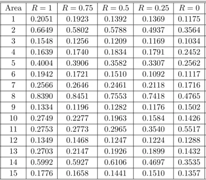
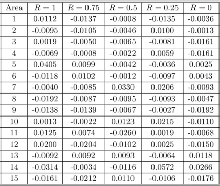
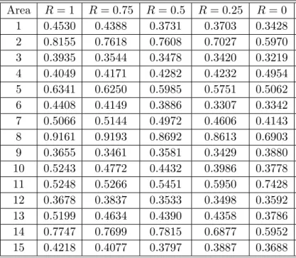
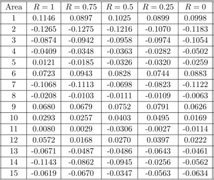
Table E.1 Bias forθb_gR within areas 1-15 comparing to population estimatorθgpop

across different scenarios determined by the variance ratioR. . . 151 Table E.2 Bias forθb_gR within areas 16-30 comparing to population estimatorθ_gpop

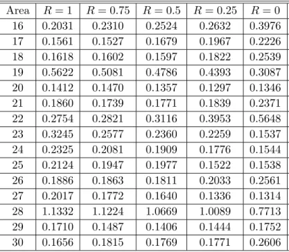
across different scenarios determined by the variance ratioR. . . 152 Table E.3 Variance forθgRb within areas 1-15 across different scenarios determined

by the variance ratioR. . . 152 Table E.4 Variance forθgRb within areas 16-30 across different scenarios determined

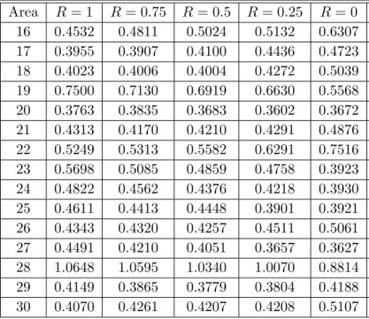
by the variance ratioR. . . 153 Table E.5 Root mean square error within areas 1-15 comparing to population

estimator θgpop across different scenarios determined by the variance ratioR. . . 153 Table E.6 Root mean square error forθb_gR within areas 16-30 comparing to

popu-lation estimatorθgpop across different scenarios determined by the vari-ance ratioR. . . 154 Table E.7 Bias forθgRb within areas 1-15 comparing to true mean of areaθgT across

different scenarios determined by the variance ratioR. . . 155 Table E.8 Bias for θb_gR within areas 16-30 comparing to true mean of area θ_gT

across different scenarios determined by the variance ratioR. . . 156 Table E.9 Root mean square error for θb_gR within areas 1-15 comparing to true

mean of area θgT across different scenarios determined by the variance

ratioR. . . 156 Table E.10 Root mean square error for θb_gR within areas 16-30 comparing to true

mean of area θgT across different scenarios determined by the variance

ratioR. . . 157 Table E.11 Bias forθb_gRwithin areas 1-15 comparing to area meanθ_gacross different

scenarios determined by the variance ratioR. . . 157 Table E.12 Bias for θgRb within areas 16-30 comparing to area mean θg across

(24)

Table E.13 Root mean square error for θb_gR within areas 1-15 comparing to area

meanθg across different scenarios determined by the variance ratioR. 158 Table E.14 Root mean square error for θb_gR within areas 16-30 comparing to area

meanθg across different scenarios determined by the variance ratioR. 159 Table E.15 Bias forθgFb within areas 1-15 comparing to population estimatorθgpop

across different scenarios determined by the variance ratioR. . . 160 Table E.16 Bias forθgFb within areas 16-30 comparing to population estimatorθgpop

across different scenarios determined by the variance ratioR. . . 161 Table E.17 Variance forθb_gF within areas 1-15 across different scenarios determined

by the variance ratioR. . . 161 Table E.18 Variance θb_gF within areas 16-30 across different scenarios determined

by the variance ratioR. . . 162 Table E.19 Root mean square error for θgFb within areas 1-15 comparing to

popu-lation estimatorθgpop across different scenarios determined by the

vari-ance ratioR. . . 162 Table E.20 Root mean square error forθgFb with within areas 16-30 comparing to

population estimatorθgpop across different scenarios determined by the

variance ratioR. . . 163 Table E.21 Bias forθb_gF within areas 1-15 comparing to true mean of areaθ_gT across

different scenarios determined by the variance ratioR. . . 164 Table E.22 Bias for θgFb within areas 16-30 comparing to true mean of area θgT

across different scenarios determined by the variance ratioR. . . 165 Table E.23 Root mean square error for θb_gF within areas 1-15 comparing to true

mean of area θgT across different scenarios determined by the variance ratioR. . . 165 Table E.24 Root mean square error for θgFb within areas 16-30 comparing to true

mean of area θgT across different scenarios determined by the variance ratioR. . . 166

(25)

Table E.25 Bias forθb_gF within areas 1-15 comparing to area meanθgacross different

scenarios determined by the variance ratioR. . . 166 Table E.26 Bias for θb_gF within areas 16-30 comparing to area mean θ_g across

dif-ferent scenarios determined by the variance ratioR. . . 167 Table E.27 Root mean square error for θgFb within areas 1-15 comparing to area

meanθg across different scenarios determined by the variance ratioR. 167

Table E.28 Root mean square error for θgFb within areas 16-30 comparing to area

meanθg across different scenarios determined by the variance ratioR. 168

Table E.29 Bias forθb_{gF p}within areas 1-15 comparing to population estimatorθ_gpop

across different scenarios determined by the variance ratioR. . . 169 Table E.30 Bias for θb_{gF p} within areas 16-30 comparing to population estimator

θgpop across different scenarios determined by the variance ratioR. . . 170

Table E.31 Variance forθgF pb within areas 1-15 across different scenarios determined

by the variance ratioR. . . 170 Table E.32 Variance for θgF pb within areas 16-30 across different scenarios

deter-mined by the variance ratioR. . . 171 Table E.33 Root mean square error forθb_{gF p} within areas 1-15 comparing to

popu-lation estimatorθgpop across different scenarios determined by the vari-ance ratioR. . . 171 Table E.34 Root mean square error forθb_{gF p}within areas 16-30 comparing to

popu-lation estimatorθgpop across different scenarios determined by the vari-ance ratioR. . . 172 Table E.35 Bias for θb_{gF p} within areas 1-15 comparing to true mean of area θ_gT

across different scenarios determined by the variance ratioR. . . 173 Table E.36 Bias for θb_{gF p} within areas 16-30 comparing to true mean of area θ_gT

(26)

Table E.37 Root mean square error for θb_{gF p} within areas 1-15 comparing to true

mean of area θgT across different scenarios determined by the variance ratioR. . . 174 Table E.38 Root mean square error for θgF pb within areas 16-30 comparing to true

mean of area θgT across different scenarios determined by the variance ratioR. . . 175 Table E.39 Bias for θgF pb within areas 1-15 comparing to area mean θg across

dif-ferent scenarios determined by the variance ratioR. . . 175 Table E.40 Bias for θb_{gF p} within areas 16-30 comparing to area mean θ_g across

different scenarios determined by the variance ratioR. . . 176 Table E.41 Root mean square error for θb_{gF p} within areas 1-15 comparing to area

meanθg across different scenarios determined by the variance ratioR. 176 Table E.42 Root mean square error forθgF pb within areas 16-30 comparing to area

(27)

CHAPTER 1. Robust Small Area Estimation for the Fay-Herriot Model

Small area estimation has long been a popular and important research topic in survey statistics. The research is predominantly based on normality assumptions of the associated stochastic variables. We consider here the basic area level model, popularly known as Fay-Herriot model, and make inference without any distributional assumptions with the exception of a few moment assumptions. In the process, we propose a new method of model parame-ter estimation, study its statistical properties and use the resulting parameparame-ter estimators as components in small area estimators. The second order approximation of the mean squared error of the proposed small area estimators is derived, and we also describe a second order correct estimator of the mean squared error. While our asymptotic expansions do not follow the standard approach, the existing results under specific distributional assumptions can be derived as special cases of our general result. A numerical study shows the usefulness of this new theory, particularly for non-normal situations.

1.1 Introduction

The purpose of this chapter is to develop nonparametric inference for small area means when only area level summary statistics are available. Small-area estimation is important in survey applications, particularly in those fields of official statistics where legislative mandates require socioeconomic estimates within jurisdictions narrower than can accurately be described by direct estimates from national surveys. Prediction based on the Fay-Herriot model (FH) (Fay and Herriot, 1979) is one of the most popular techniques in small area estimation. Model estimates and predictions are simple, well studied and easy to implement via standard software likeSAS. Another important advantage of the FH model is that it only requires summary data,

(28)

not elemental-level data that might be unavailable to the analyst because of confidentiality concerns.

The Fay-Herriot model has two stochastic variables, one for the sampling error and the other one representing small area specific random effects. These two random variables and a fixed effect linear regression are additively related to the design based estimators of small area means. The best linear unbiased predictor (BLUP) is commonly used as the small area estimator, and construction of the BLUP does not require any distributional assumption. However, the BLUP is a function of model parameters, and thus their estimated values are plugged-in before the BLUP can be used. The resulting plug-in estimators are known as empirical or estimated best linear unbiased predictor (EBLUP).

A number of estimation procedures exist for the model parameters of the FH model. For example, the method of moments used by Prasad and Rao (1990), maximum-likelihood (ML) and restricted maximum likelihood (REML) used by Datta et al.(2000), and the Fay-Herriot method used by Fay and Herriot (1979) and then studied by Dattaet al.(2005). The variance parameter estimates by the method of moments (Prasad and Rao, 1990), and that in the Fay-Herriot method used by Fay and Herriot (1979) do not requires normality, and both lead to consistent estimators as sample size increases to infinity. Jiang (1996) established the consistency and asymptotic normality for REML parameter estimators without normality assumption, and also provide the necessary and sufficient conditions for the similar MLE asymptotic properties.

The mean square prediction error estimation (MSPE) is an integral part of small area estimation research. See Rao (2003) for details. MSPE estimation depends on the method of model parameter estimation, but also on the assumptions made about the distributions of the random model components. Under normal distribution assumptions, Prasad and Rao showed the result for the method of moments (Prasad and Rao, 1990), restricted maximum likelihood (REML) result is showed by Datta et al. (2000), and Fay-Herriot method result is showed by Datta et al. (2005). Lahiri and Rao (1995) showed that the MSPE estimators of Prasad and Rao (1990) are valid under nonnormality of random effects distribution. The method of

(29)

moments and Fay-Herriot method robustness with nonnormality assumptions for two variables distribution are shown in Chenet al. (2007).

In some applications, it has been noted that the sampling error distribution may not be normal and this might have significant impact on MSPE estimation. For example, see Wang and Fuller (2003), Hall and Maiti (2007) and the simulation study of Prasad and Rao (1990). Also, different model parameter estimation methods may perform differently even under nor-mality depending on the ratio of small area specific model variance to the sampling variance. See the simulation study of Datta et al. (2000) and Datta et al. (2005). These motivate us to develop a robust small area estimation method where we do not require any distributional assumption on the random components, but instead only require the existence of a number of finite moments. In the process, we also develop a new method of model parameter estimation which is approximately as efficient as existing methods of estimation under normality and more efficient under departures from normality.

In the next section, we describe the model and small area parameter estimation along with their asymptotic properties. The approximation of the prediction mean squared error is provided in Section 1.3, and Section 1.4 provides the estimators of the MSPE. Technical details are deferred to the Appendix.

1.2 The FH Model and Small Area Estimation

Let y1, y2, . . . , yn be observations, and x1,x2, . . . ,xn be fixed predictors. Then the FH

model is defined as

yi =xT_i β+ui+εi, i= 1, . . . , n, (1.1)

where β= (β1, . . . , βp)T is ap×1 vector of regression coefficients. The area specific random effects ui are assumed to be independent and identically distributed (iid) with E(ui) = 0 and Var(ui) =σu2(≥0). The sampling errorsi are also independently distributed with mean zero

(30)

Small area estimates (SAE’s) based on such FH models are statistics designed to estimate the parameters

θi = xTi β + ui, i = 1, . . . , n. (1.2)

In a typical survey application, the values yi are direct survey estimators of the target small-area parameters θi in the sampled area’s but may be unacceptably variable because of small

sample size in some or all the small areas. The Di represent the sampling variance of the yi

and are required to be known (or at least estimated with very high accuracy) from an outside source, for instance the statistical agency responsible for collecting the survey data. If the remaining parameters were also known, the SAE’s would be the BLUP’s and are given by

˜ θi=xT_i β+γi(yi−xT_i β), i= 1,· · ·, n, (1.3) where γi = σu2 σ2 u+Di. Since σ 2

u,β are unknown, BLUP’s are not usable until we estimate these

model parameters.

1.2.1 Model Parameter Estimation

We propose an iterative method of parameter estimation based on the method of moments. It does not require the normality assumption and enjoys similar asymptotic properties as existing methods mentioned in Section 1. Under the following transformation,

y_i∗ = √yi Di x∗_i = √xi Di Y∗ = (y∗₁, . . . , y∗_n)T X∗ = (x∗₁T, . . . ,x∗_nT)T.

The estimators of βand σ2_u are defined as the solution to the following system of equations:

     β = (X∗TX∗)−1X∗TY∗−Pn_i₌₁x∗_i σ2u σ2 u+Di(y ∗ i −x∗iTβ) σ_u2 = 1_nPn_i₌₁ σu2 σ2 u+Di(yi−x T i β)2 . (1.4)

(31)

1. Compute βb (0) andσ_b2(0)u : b β(0) = ( n X i=1 xixTi ) −1₍ n X i=1 xiyi) = (XTX)−1(XTY) b σ_u2(0) = max( 1 n−p[ n X i=1 (yi−xT_i βb (0) )2− n X i=1 Di(1−˜hii)],0), where ˜ hii = xTi ( n X i=1 xixTi )−1xi. 2. Compute βb (j) forj≥1: b β(j) = ( n X i=1 x∗_ix∗_iT)−1( n X i=1 x∗_iyb ∗(j−1) i ) = (X∗TX∗)−1(X∗TcY ∗(j−1) ), with b u(_ij−1) = bσ 2(j−1) u b σ2(uj−1)+Di (yi−xTi βb (j−1) ) b y_i∗(j−1) = yi−ub (j−1) i √ Di . 3. Compute σb 2(j−1) u forj ≥1: b σ2(_uj)= 1 n X σ_b 2(j−1) u b σu2(j−1)+Di (yi−xT_i βb (j) )2.

4. If the current value of the estimators βb (j)

and σb 2(j)

u are sufficiently close to the

previ-ous value βb (j−1)

and σb 2(j−1)

u , stop iterations and use the current estimates as the final

(32)

As initial values in step (1) of the algorithm, we have used the OLS estimator for β and the PR moment estimator forσ2_u, but other consistent estimators would work here as well. We will show that the proposed parameter estimators βb and σ_b2_u enjoy some desirable theoretical

properties including √n-consistency. We make the following assumptions:

A1 The matrix (1_nXTX)−1 isO(1) element-wise, and

sup i ˜ hii=xT_i ( n X i=1 xixTi ) −1_x i=O(n−1).

A2 The quantities xi, σu2, Di are bounded, and Di > γ1≥0, σu2 > γ2≥0.

A3 For s≤8, E(ui+εi)2s exists and is bounded.

Theorem 1.2.1 Under Assumptions A1, A2 and A3, the estimators βb and b

σ_u2 are consistent for the parameters β and σ_u2 in model (1.1), in the sense that:

b

β = β+1p×Op(n−1/2)

b

σ_u2 = σ_u2+Op(n−1/2), (1.5)

where 1p is thep×1 vector (1, . . . ,1)T.

The proof of Theorem 1.2.1 is provided in Appendix A.

Theorem 1.2.2 Under Assumption A1, A2 and A3, the asymptotic distribution of βb and _bσ2

is V−12        b β−β b σ_u2−σ2_u        L → N(0,Ip+1), where V =        V_ββT V β_σ2 u VT_β_σ2 u Vσ 2 uσ2u        ,

(33)

V_ββT = ( n X i=1 xixTi σ2 u+Di )−1 V_σ2 uσu2 = ( n X i=1 σ_u2 σ2 u+Di )−2 n X i=1 σ_u4 (σ2 u+Di)2 Var((ui+εi)2) V βσ2 u = 1 n( n X i=1 xixTi σ2 u+Di )−1 n X i=1 xiσ_u2 (σ2 u+Di)2 ×Covui+εi,(ui+εi)2 1 n n X i=1 σ_u2 (σ2 u+Di)2 !−1 ,

and Ip+1 is the(p+ 1)×(p+ 1) identity matrix.

The Proof of Theorem 1.2.2 uses the Linderberg Central Limit Theorem and is given in Appendix A.

In order to use Theorem 1.2.2 for inference for the parameters, we need to estimate the elements of V. We propose to use the following simply plug-in estimators for _{V ββ},V_σ2

uσu2 and _{V β}_σ2 u, respectively: c V ββ = ( n X i=1 xixTi b σ2 u+Di )−1 c V_σ2 uσ2u = n (Pn_i₌₁ 1 b σ2 u+Di) 2 " 1 n( n X i=1 (yi−xT_i βb)4 (σbu2+Di)2 )−1 # c V βσ2 u = n X i=1 xixTi b σ2 u+Di !−1 _n X i=1 xi(yi−xTi βb)3 (_bσ2 u+Di)2 n X i=1 1 b σ2 u+Di !−1 .

Theorem 1.2.3 Under Assumption A1, A2 and A3, cV ββ,cV_σ2

uσu2 and V βc σu2 are consistent

for _{V ββ}, _{V β}_σ2

u andVσ

2

uσ2u, in the sense that

ncV ββ = nV ββT +1p×1Tp ×Op(n− 1 2) ncV_σ2 uσu2 = nVσu2σu2 +Op(n −1 2) ncV β σ2 u = nV βσ2u+1p×Op(n −1 2).

The Proof of Theorem 1.2.3 is given in Appendix A.

The previous results make no assumptions about the form of the distributions of the random components. Even in that general case, the estimator forβis asymptotically equivalent to the

(34)

GLS estimator with correctly specified variance-covariance matrix, the same result as for the ML and REML estimators under normality. Rao (2003) provides the asymptotic covariance matrix under normality assumption in page 100 and page 120. It is also easy to see that, if both errors are normally distributed, the components of the asymptotic variance matrix in Theorem 1.2.2 reduce to:

V_ββT = ( n X i=1 xixTi σ2 u+Di )−1 V_σ2 uσu2 = 2n( n X i=1 1 σ2 u+Di )−2 V βσ2 u = 1×0,

where1is thep×1 vector (1, . . . ,1)T. Hence, the estimatorsβb andσ_b_u2 become asymptotically

independent, as found for the ML and REML estimators ((Rao, 2003), p100). Furthermore, the asymptotic variance forσb

2

u is the same as that obtained for the FH estimator by Datta et

al.(2005).

1.2.2 Finite Sample Performance

We conducted an extensive simulation study evaluating the proposed parameter estimators and associated inference measures, with complete results available in Appendix B.

We simulated data using the FH model (1.1). The xi are taken to be univariate and

are generated from the standard normal distribution N(0,1), and then held fixed across the simulations. Theβ0 andβ1have true parameter values set at (0.5, 1). Theui, εi are generated under several distributions and withσ2

u= 1 and several scenarios for theDi. Following Datta

et al.(2005), we split the sample into five equal-sized groups with equal sampling variance Di

in each group, and consider three different patterns ofDi’s: (a) 0.7, 0.6, 0.5, 0.4, 0.3; (b) 2.0, 0.6, 0.5, 0.4, 0.2; (c) 4.0, 0.6, 0.5, 0.4, 0.1. We investigated the following distributions for the random components, suitably standardized to achieve the desired variances:

1. Both ui and εi from normal distributions,

2. The εi from normal distribution, ui from centered chi-square distribution with 0 and

(35)

3. Both ui and εi from centered chi-square distributions with 0 and degrees of freedom = variance / 2,

4. The εi from normal distribution,ui from t distribution with df=3,

5. Both ui and εi from t distribution with df=3.

We simulated sample sizes n = 15,30,60,240,1000, and for each scenario, the number of replicates was 1000. The following estimators were investigated:

1. Estimation by the Robust Estimator (RE) algorithm in Section 1.2.1: σ_b2 u,βb,

2. Fay-Herriot estimation (Fay and Herriot, 1979) forσ_u2, and GLS estimation forβ: σ_b2_{uF H},βb_{F H},

3. MME estimation (Prasad and Rao, 1990) forσ_u2, and GLS estimation forβ: bσ 2

uM M E,βb_{M M E},

4. REML estimation (Dattaet al., 2000) forσ_u2, and GLS estimation forβ: σb 2

uREM L,βb_{REM L}.

In the latter three cases, the GLS estimators were computed with estimated variance compo-nents.

Tables B.1 to B.60 display the bias, root mean square error forβandσ_u2, estimated standard deviation, coverage probabilities and coverage length of nominal 95% confidence intervals for

σ_u2 for Robust Estimation (RE), Fay-Herriot estimation, MME estimation, REML estimation across different distribution scenarios. We investigated the coverage properties of the confidence intervals forσ2_u obtained using the asymptotic normal distribution of the estimators and their asymptotic variance estimators. For all other methods, we plugged in the estimates for theσ_u2

in the asymptotic variance formula under normality assumptions.

We first investigated the bias, variance and mean squared error properties of these esti-mators of the parametersβb. Interestingly, all the methods considered lead to estimators with

similar properties, with no estimator consistently dominating the others in any of the scenarios. Specifically, the bias and root mean squared error for estimators of β₀ and β₁ displayed no substantial differences under normal or nonnormal distribution assumptions. As the sample size increases, the bias and root mean squared error for estimators ofβ₀ and β₁ decreases for all estimators with different patternDi.

(36)

For the estimators of σ2_u, some difference in bias, root mean square error were seen, but no estimator was consistently better than other estimators across the different scenarios. As the sample size increases, the bias and root mean squared error for estimators ofσ_u2 decreases for all estimators with different pattern Di that show no significant difference for different methods. The most significant difference appears in two things: one is the difference between root mean square error and estimated standard deviation of σ2_u, the other one is the cov-erage probabilities of nominal 95% confidence intervals for σ_u2 for different sample sizes and the distribution scenarios. The results show the difference between root mean square error and estimated standard deviation and the undercoverage of the proposed method decreases steadily and eventually disappears for n= 1000 for non-normal distributions for the random components and different patterns of the Di, while for all other methods, the difference and

the undercoverage still remain as the sample size increases.

Normal distribution Chi-square distribution

RE FH MME REML RE FH MME REML

n= 15 0.739 0.866 0.869 0.822 0.515 0.508 0.513 0.471

n= 30 0.846 0.914 0.912 0.896 0.647 0.482 0.492 0.457

n= 60 0.896 0.928 0.929 0.919 0.748 0.485 0.476 0.479

n= 240 0.943 0.947 0.949 0.947 0.865 0.486 0.503 0.472

n= 1000 0.957 0.961 0.962 0.957 0.93 0.508 0.506 0.506 Table 1.1 Coverage probabilities for nominal 95% confidence intervals

us-ing asymptotic normality and estimated variances for four dif-ferent estimators: Robust Estimation (RE), Fay-Herriot estima-tion, MME estimaestima-tion, REML estimaestima-tion, when both ui and εi are normal or centered chi-square distribution forDi in pat-tern(a).

Table 1.1 displays the coverage probabilities of nominal 95% confidence intervals for σ_u2

for different sample sizes and two distribution scenarios, for the case with the Di following pattern (a). The left-hand side shows the coverage probabilities when both ui and εi are

normally distributed, while the right-hand size displays the results when both components follow centeredχ2 distributions. The results show that the proposed method results in modest undercoverage compared to the three other methods when the errors are normally distributed,

(37)

with most of the undercoverage disappearing whenn= 60 or higher. In contrast, all methods result in severe undercoverage when the errors follow χ2 and the sample size is small. While the undercoverage of the other three method remains large and stable with increasing sample size, the undercoverage of the proposed method decreases steadily and eventually disappears forn= 1000. Similar results were obtained for other non-normal distributions for the random components and patterns of theDi.

Overall, the bias, variance and mean squared error properties of these estimators of the parametersβb andσ_u2 perform similarly for different estimators under different scenarios.

How-ever, in the case of σ_u2, the behavior of the different estimators depended significantly on the distributions of the random components. The coverage probabilities of nominal 95% confidence intervals forσ2_u for different sample sizes and nonnormal distribution scenarios perform signifi-cant different as sample size increases, which shows that the proposed estimator is robust to a wide range of random component distributions, and only results in a modest loss of efficiency when the normality assumption is correct.

1.3 Mean Squared Prediction Error of EBLUP

We now turn to the problem of estimating the small area parameters θi in (1.2). When

we replace the unknown parameters in the BLUP ˜θi in (1.3) by the estimators defined in the

previous section, we obtain the Empirical BLUP (EBLUP)

b θi =xT_i βb + b σ2_u b σ2 u+Di (yi−xT_i βb), i= 1,· · ·, n.

The uncertainty of the EBLUP is usually measured by its mean squared prediction error (MSPE) and is defined asE(θb_i−θ_i)2, i= 1,· · ·, n. When regularity conditions and normality

of the errors hold, it reduces to

M SP E(θb_i)≈g₁+g₂+g₃,

where we define

(38)

g2 = (1−γi)2xTi V_ββTxi (1.7) g3 = (1−γi)2 1 (σ2 u+Di) V_σ2 uσ2u, (1.8)

which are same as theg1, g2, g3 in Rao (2003) when both distributions are normal, and

γi =σu2/(σu2+Di). (1.9)

For convenience, we also define ξu1 and ξu2 as skewness and kurtosis of ui, ξe1i and ξe2i as

skewness and kurtosis of εi. It is well known that there is no exact expression for the MSPE even when all the random components are normal, and a second order approximation is a standard practice for small area research. A second order approximation is required in order to fully account for the estimation of the model parameters, in addition to the uncertainty of the prediction itself (i.e. the difference betweenθi and ˜θi). To achieve this goal, we first define

the approximating random variable θ_i∗ as

θ∗_i = xT_iβ+ σ 2 u σ2 u+Di (ui+εi) + Di σ2 u+Di xT_i ( n X i=1 xixTi σ2 u+Di )−1 n X i=1 xi(ui+εi) σ2 u+Di + Di (σ2 u+Di)2 (ui+εi)( n X i=1 1 σ2 u+Di )−1 ( _n X i=1 (ui+εi)2 σ2 u+Di −n ) = θi˜ + (1−γi)xT_i ( n X i=1 xixTi σ2 u+Di )−1 n X i=1 xi(ui+εi) σ2 u+Di +(1−γi) 1 σ2 u+Di (ui+εi)( n X i=1 1 σ2 u+Di )−1 ( _n X i=1 (ui+εi)2 σ2 u+Di −n ) .

In the following two theorems, we first obtain an approximation to the MSPE of θ∗_i, and then show that the MSPE of θib is second order equivalent to E(θ_i∗−θi)2.

Theorem 1.3.1 Under Assumption A1,A2 and A3, the following approximation holds: E(θ∗_i −θi)2=g1+g2+g3

+2(1−γi)2γ2_i(

n X

i=1

γi)−1nξe2i×Di−ξu2×σ2u o

(39)

Theorem 1.3.2 Under Assumption A1,A2 and A3, an approximation forM SP E(θib)is given

by

E(θb_i−θ_i)2 = E(θ∗_i −θ_i)2+O(n−2).

The Proofs of Theorems 1.3.1 and 1.3.2 are given in Appendix A.

In the approximation of Theorem 1.3.1, the first three terms match the form of the leading terms usually denoted asg1, g2, g3 from other methods as in Rao (2003). Only the asymptotic variance forσb

2

u differs from that obtained under other estimation methods.

The fourth term in the approximation of Theorem 1.3.1 is due to the fourth moments of the random components. That term is not present when ui, εi are both normal, since

Eu4_i = 3σ_u4,Eε4_i = 3D2_i. In that case, the approximation reduces to

E(θb_i−θ_i)2 = g₁+g₂+ 2n(1−γi)2 (σ2 u+Di) ( n X i=1 1 σ2 u+Di )−2+O(n−2) = g1+g2+g3+O(n−2),

which is same result as for the FH estimator when ui, εi are both normal (Dattaet al., 2005).

1.4 Estimation of Mean Squared Prediction Error

1.4.1 Mean Squared Prediction Error Estimation

The MSPE approximation of Theorem 1.3.1 is not directly usable for inference because it involves the unknown model parameters. The seminal work of Prasad and Rao (1990) shows that replacing the parameters by their estimates is not enough because it leaves a bias of order

O(n−1). As before, there is no exact expression for this bias and thus further approximation needed.

The estimator we propose is defined as follows:

mspe(θb_i) = Diσb 2 u b σ2 u+Di + ( Di b σ2 u+Di )2xT_i cV ββTx_i+ 2( Di b σ2 u+Di )2 1 (σ_b2 u+Di) c V_σ2 uσu2 +( Di b σ2 u+Di )2( n X i=1 1 b σ2 u+Di )−1 n X i=1 xT_i (σb 2 u+Di) ( n X i=1 xixTi b σ2 u+Di )−1xi

(40)

+( Di b σ2 u+Di )2( n X i=1 1 b σ2 u+Di )−2 n X i=1 1 (σbu2+Di) ((yi−x T i βb)4 (σbu2+Di)2 −1) −( Di b σ2 u+Di )2( n X i=1 1 b σ2 u+Di )−3 n X i=1 1 (σb 2 u+Di)2 n X i=1 ((yi−x T i βb)4 (bσ 2 u+Di)2 −1) +2 D 2 iσb 2 u (σb 2 u+Di)4 ( n X i=1 1 b σ2 u+Di )−1n3σb 2 u−3Di o + 2 Diσb 2 u (σb 2 u+Di)4 ( n X i=1 1 b σ2 u+Di )−1Fi −2 D 2 i (σb 2 u+Di)4 ( n X i=1 1 b σ2 u+Di )−1n(yi−xT_i βb)4−Fi−6σ_b2_uDi o ,

where Fi = E(ε4i) is assumed known. The following theorem shows that mspe(θb_i) is second

order correct for the MSPE ofθib.

Theorem 1.4.1 Under Assumption A1,A2 and A3,

E(mspe(θb_i)) = MSPE(θb_i) +O(n−2).

The Proof of Theorem 1.4.1. is given in Appendix A. And it will be in the form that

g1 = E Diσb 2 u b σ2 u+Di + E[ Di b σ2 u+Di ]2 1 (σb 2 u+Di) d A.Var(σb 2 u−σu2) +E( Di b σ2 u+Di )2( n X i=1 1 b σ2 u+Di )−1 n X i=1 xT_i (bσu2+Di) ( n X i=1 xixTi b σ2 u+Di )−1xi +E( Di b σ2 u+Di )2( n X i=1 1 b σ2 u+Di )−2 n X i=1 1 (_bσ2 u+Di) ((yi−x T i βb)4 (σ_b2 u+Di)2 −1) −E( Di b σ2 u+Di )2( n X i=1 1 b σ2 u+Di )−3 n X i=1 1 (bσ 2 u+Di)2 n X i=1 ((yi−x T i βb)4 (σb 2 u+Di)2 −1) +O(n−2), g2 = E( Di b σ2 u+Di )2xT_i cV ββTxi+O(n −2₎_,

(41)

g3 = E2( Di b σ2 u+Di )2 1 (σbu2+Di) c V_σ2 uσu2 +O(n −2₎_, (1−γi)2γi2( n X i=1 γi)−1 n ξe2i×Di−ξu2×σ2u o = E D 2 ibσ 2 u (σb 2 u+Di)4 ( n X i=1 1 b σ2 u+Di )−1n3σb 2 u−3Di o + Dibσ 2 u (σb 2 u+Di)4 ( n X i=1 1 b σ2 u+Di )−1Eε4_i −E D 2 i (σb 2 u+Di)4 ( n X i=1 1 b σ2 u+Di )−1n(yi−xT_i βb)4−Eε4_i −6_bσ_u2Di o +O(n−2).

When both ui andεi are normally distributed, we can simplifymspe(θb_i) as

mspe(θb_i) = Diσb 2 u b σ2 u+Di + ( Di b σ2 u+Di )2xT_i( n X i=1 xixTi b σ2 u+Di )−1xi+ 4nD2_i (σb 2 u+Di)3 ( n X i=1 1 b σ2 u+Di )−2 +( Di b σ2 u+Di )2( n X i=1 1 b σ2 u+Di )−1 n X i=1 xT i (σb 2 u+Di) ( n X i=1 xixTi b σ2 u+Di )−1xi +2( Di b σ2 u+Di )2( n X i=1 1 b σ2 u+Di )−1−2n( Di b σ2 u+Di )2( n X i=1 1 b σ2 u+Di )−3 n X i=1 1 (σb 2 u+Di)2 .

One notable difference between our estimator for the MSPE and that of other authors is the requirement for the fourth moment Fi of the sampling errors to be known. Under the assumption of normally distributed sampling errors, this is not explicitly required because the fourth moment is related toDi. But just like knowledge ofDi is required in order to construct an EBLUP for θi under the FH model, knowledge of the fourth moment is needed order to

estimate the MSPE of the EBLUP. The fourth moment ofui also appears in the approximation

of Theorem 1.3.1, but once Fi is known, it can be estimated based on the sample residuals (yi−xTi βb). In principle, the survey organization providing theD_i could also be requested to

provide theFi, since for many designs these can be estimated consistently. In practice however, it will often be necessary to obtain the Fi through other means.

(42)

1.4.2 Finite Sample Performance

We have performed an extensive simulation study to evaluate the finite sample performance of the proposed EBLUP and its associated MSPE estimator under a variety of situations, with the results described in Appendix B. We discuss some of the results here.

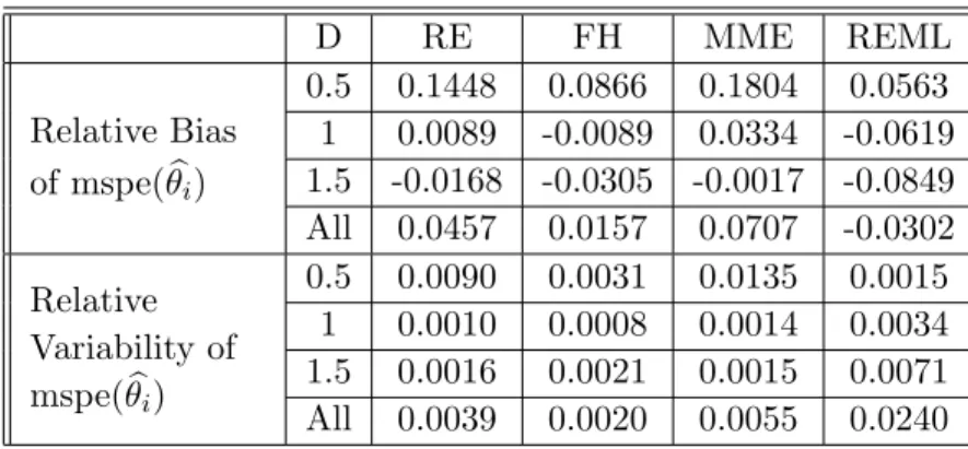
The small areas are divided into three equal-sized groups, and we consider four different patterns of sampling variances across the groups, namely (a) 0.5, 1, 1.5; (b) 0.9, 0.5, 0.3; (c) 1, 1.5, 2; (d) 0.1, 0.5, 4. We consider the following distributions: (i) bothui and εi from normal

distributions; (ii) both ui and εi from centered chi-square distributions with 0 and degrees of

freedom as variance / 2 and (iii) both ui and εi from centered exponential distributions. The variance ofuiis set at 1. The sample sizes (in each replicate, the number of observations) used

in the simulation aren= 15,30 and the number of replicates for each scenario is 1000. The model is totally same as the previous one, the only difference is that we change the patterns of sampling variances across the groups as (a), (b), (c), (d).

We restrict our comparison to the FH estimator because FH found to be the smallest relative bias among all available methods of MSPE estimators (Datta et al., 2005).

In table 1.2, along with the overall mean the group means are also provided. When the sampling variance is less than the model variance, the FH method perform better (with smaller relative bias and relative variability of mspe(θb_i)). But the proposed method performs much

better compare to FH when the sampling variance is higher than the model variance. In Datta

et al. (2005) the FH method was particularly good when the sampling variance was much higher than the model variance. Thus our proposed method working in the same direction of FH method under non-normal situation.

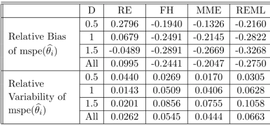
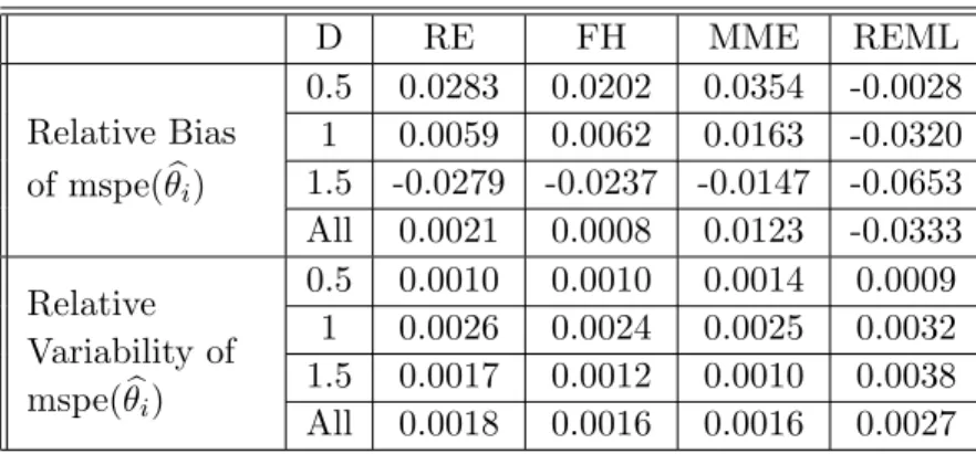
In the Appendix B, detailed performance comparing Bias and MSPE of θib, Relative Bias

and Relative Variability of mspe(θb_i) among four different estimators across distribution

sce-narios are provided in Tables B.61 to B.84. Under the normal situation, the proposed method doesn’t perform better (with smaller relative bias and relative variability of mspe(θb_i))

com-paring with other methods. Under the non-normal situations, the proposed method performs much better comparing to other methods under some pattern of D. When D is in pattern (a)

(43)

n=15 n=30 D RE FH RE FH Bias of θib 0.5 -0.0100 -0.0109 -0.0035 -0.0032 1 -0.0087 -0.0076 -0.0047 -0.0050 1.5 -0.0235 -0.0226 0.0067 0.0061 All -0.0141 -0.0137 -0.0005 -0.0007 MSPE ofθb_i 0.5 0.3869 0.3693 0.4431 0.4300 1 0.7665 0.7595 0.6579 0.6537 1.5 0.8883 0.8939 0.8358 0.8350 All 0.6806 0.6742 0.6456 0.6395

Relative Bias of mspe(θb_i)

0.5 0.7094 0.1983 0.2796 -0.1940 1 0.0123 -0.2715 0.0679 -0.2491 1.5 0.0115 -0.2372 -0.0489 -0.2891 All 0.2444 -0.1035 0.0995 -0.2441

Relative Variability of mspe (θib)

0.5 0.2088 0.0295 0.0440 0.0269 1 0.0113 0.0681 0.0143 0.0509 1.5 0.0324 0.0797 0.0201 0.0856 All 0.0842 0.0591 0.0262 0.0545 Table 1.2 Bias and MSPE of θib, Relative Bias and Relative Variability of

mspe(θib) for Robust Estimation (RE), Fay-Herriot estimation

when both ui and εi are Chi-squared distribution and D is

pat-tern (a).

and the sampling variance is less than the model variance, our proposed method doesn’t per-form advantage in nonnormality situations. But the proposed method perper-forms much better when the sampling variance increases. Similar situation appears when D is in pattern (b) that the proposed method performs much better when the sampling variance increases to close to the model variance. When D is in pattern (c) and random components are centered expo-nential distributions, the proposed method performs much better when the sampling variance increases to bigger than the model variance when n is 15. The proposed method performs much better when the sampling variance increases to bigger than the model variance when D is in pattern (c) and random components are centered Chi-Squared or Exponential distributions and n is 30. When D is in pattern (d), the sampling variances distribute very unbalanced. The proposed method doesn’t perform better comparing with other methods.