Revisiting activity sampling: A fresh look at binomial proportion confidence intervals

(1)

This is the author’s version of a work that was submitted to / accepted for publication. Citation for final published version:

Disney, Stephen Michael 2016. Revisiting activity sampling: A fresh look at binomial proportion confidence intervals. European Journal of Industrial Engineering 10 (6) , pp. 724-759.

10.1504/EJIE.2016.081021 file

Publishers page: http://dx.doi.org/ 10.1504/EJIE.2016.081021 <http://dx.doi.org/ 10.1504/EJIE.2016.081021>

Please note:

Changes made as a result of publishing processes such as copy-editing, formatting and page numbers may not be reflected in this version. For the definitive version of this publication, please refer to the published source. You are advised to consult the publisher’s version if you wish to cite

this paper.

This version is being made available in accordance with publisher policies. See

http://orca.cf.ac.uk/policies.html for usage policies. Copyright and moral rights for publications made available in ORCA are retained by the copyright holders.

(2)

Revisiting activity sampling:

a fresh look at binomial proportion confidence intervals

Stephen M. Disney

Logistics Systems Dynamics Group, Cardiff Business School, Cardiff University. Email: [email protected]. Telephone: +44(0)2920 876310.

Abstract

The Wald interval is typically used to assign confidence to the accuracy of activity sampling studies. It is known the performance of the Wald interval is poor, especially when the observed probability is near zero or one. The suitability of the Wald interval for activity sampling is not often discussed in the operations management literature; if it is, this is usually followed by inappropriate and incorrect advice. Herein a range of alternative binominal confidence intervals for activity sampling is reviewed. A number of selection criteria are considered including achievement of the target nominal coverage probability, size of the interval, and ease of use and presentation. It is recommended that the Clopper-Pearson interval is used for activity sampling. A table of confidence intervals and sample sizes that is specifically designed to be used within a new activity sampling procedure based on the Clopper-Pearson interval is developed. Finally, pedagogical issues are considered.

Key words

Activity sampling, work sampling, binomial proportion confidence intervals, coverage probability.

1. Introduction and motivation

Activity sampling is an empirical data collection technique attributed to Tippet (1935). It

can be used to determine the proportion of time: an activity is being conducted by an operator; an operator is doing productive, value adding work; a machine or operator being delayed, or whether an entity (customer, supplier, product) possesses a particular (quality) characteristic or not.

Activity sampling has been defined by British Standard 3138 (1992) as “A technique in

which a large number of observations are made over a period of time of one group of machines, processes or workers. Each observation records what is happening at that instant and the percentage of observations recorded for a particular activity or delay is a measure of the percentage of time during which that activity or delay occurs”. Activity

sampling has also been known as: work sampling in the U.S.; snap reading, Tippets’

original name for the technique; the ratio delay technique, as it can be used to ascertain

the proportion of time a machine or operator is delayed or idle; and in the service sector,

random moment studies.

Activity sampling is a relatively inexpensive technique that can be used to determine the proportion of time spent on a particular activity. It can be applied to long, varied and intermittent work. It does not use a stop watch, so it is more acceptable to the subjects of the study and is not as intrusive as other methods. However, activity sampling is not efficient when activities are of a short duration, regular and predictable when time and motion studies might be more suitable.

(3)

from the study. It is known in the statistical literature that this interval is a rather poor approximation to the true interval. Herein we test this claim and find that, 80% of the time, the Wald interval does not achieve the desired confidence. This is a serious issue for anyone using activity sampling for safety assurance. To address this we review a range of alternative confidence intervals and select one for inclusion in an updated activity sampling procedure. A new procedure is recommended that actually achieves the desired confidence and accuracy levels.

1.1. The standard activity sampling procedure

For simplicity we assume that we are monitoring the types of activities that an operator is undertaking. The standard activity sampling procedure usually involves the following steps. First, a pilot study (an initial look at the situation being studied) is undertaken to ascertain the range of activities an operator undertakes. The second step is to design the sampling tour and data collection forms. The sampling tour specifies when instantaneous observations of the situation being studied are to be taken. It is assumed that the underlying probability of an activity occurring does not change over time (at least within the period of study). It is important to ensure that there is no systematic effect present in the data collected by taking observations after random intervals of time. The study period should be long enough to capture the complete range of activities the operator undertakes but the study can be interrupted if the necessary. It may be also shortened or lengthened as required. The data collection forms are simply a table with rows that note the time a observation is taken and columns that document the activity observed.

In the next step, the main data collection is undertaken. The situation being studied is observed at the prescribed moments of time and the activity being conducted by the operator is recorded in the data collection form as a tick mark. After several dozen or so observations the tick marks can be tallied to obtain an initial estimate of the probability of

an activity occurring, ˆp. Alternatively we could use judgement or experience to make an

initial estimate of ˆp . We could even believe that we are being conservative and

(incorrectly) use ˆp0.5. Note there will be a different ˆp for each of the activities. We

will not index them there – it is fairly obvious which activity is being considered as there will be a unique estimate for each of the columns in the data collection form.

Based on this initial estimate, ˆp , we can then calculate how many instantaneous

observations (n) we need to take in order to be 95% confident that the true (real, constant,

but unknown) probability of the activity occurring (p) is within a certain boundary with





2

ˆ ˆ

4 1

n p p L , (1)

where L is a tolerance of the form ˆpL, within which a desired level of accuracy has to

be achieved. Note L is an absolute distance and not a relative percentage of ˆp. L can be

thought of as the confidence interval half-width.

We continue to take the required number of observations, checking periodically with (1) for an updated value of n (which may have changed due to the new values of ˆp, the

estimate of the true probability p). Note that n will be different for each of the observed

activities (as ˆp is likely to be different for each activity). In order to gain a complete

picture of the situation, the largest n will determine the required number of samples to be

(4)

influences the trade-off between the efficiency of the procedure and the accuracy obtained.

1.2. Motivation

At first sight the activity sampling procedure seems fine. It has such a long history and is relatively straight forward, so what is the problem? Take a look at (1). What happens when L pˆ (or L 



1 pˆ



? A negative probability of p (or one that is greater than one)

is not possible, so there is an issue here. What happens when ˆp0 or pˆ 1? Equation (1)

incorrectly suggests that no samples should be taken. But rarely do operations management (OM) textbooks discuss these issues.

Equation (1) is actually a simplified and rearranged version of the so-called Wald interval

for the binomial proportion, Wald and Wolfowitz (1939). A literature review (see, for

example, Pires and Amado (2008) for a modern and particularly comprehensive treatment

of 20 different binomial proportion confidence intervals) reveals that statistical scholars have serious concerns about the adequacy of the Wald interval. However, this is the interval used in most the OM textbooks.

Table 1 summarises a review of OM books for the terms activity sampling, work

sampling, snap reading, ratio delay, random moment studies and confidence intervals. It

highlights that in general it can be said that the Wald interval is almost exclusively recommended and guidance on the interval coverage probability is limited to either a “large sample size” or “ ˆnp5 and n



1 pˆ



5”, if it is given at all. If there is indeed a problem with the Wald interval, then it means that the confidence that is assigned to the confidence interval cannot be trusted. The purpose of this paper is to investigate this issue.

1.3. Organisation of this paper

Section 2 presents a short review of the literature that exploits activity sampling to demonstrate the relevance and possible use of activity sampling. Section 3 reviews some background theory and defines notation. Section 4 studies the Wald interval. Key performance measures for confidence intervals, suitable for use in an activity sampling procedure, are defined and justified in Section 5. Section 6 studies some alternative confidence intervals from an OM activity sampling viewpoint. Section 7 reflects upon the considered confidence intervals and makes recommendations. Section 8 details a new updated activity sampling procedure that exploits the recommended confidence interval. Section 9 provides pedagogical reflections. Section 10 concludes. A blank example data collection form and the necessary tables required for the updated activity sampling procedure are presented in the appendices.

2. Recent activity sampling studies

It is interesting to quickly review studies that have used activity sampling in order to gain an understanding of the range of problems and issues that the methodology could be

applied too. Farrell et al. (2009) determined the unit labour cost of activities in a bank

across multiple branches. Tsai (1996) incorporated activity sampling into an Activity

Based Costing methodology. Thomas (1991) investigated labour productivity in the

(5)

3. Background theory and notation

Statisticians have developed several formulae to determine, with a particular level of confidence, a range of estimated probabilities that will contain the true probability. These

formulae are known as binomial proportion confidence intervals or just confidence

intervals for brevity. These confidence intervals are based on the binomial distribution as

we are concerned with the observing x number of successes (the activity occurring or not)

in n observations. Clopper and Pearson (1934) developed an exact solution and there is

also some approximate confidence intervals available that possess various properties. Let ˆp be the observed value of the probability of a particular activity occurring. This

observed value is not the true probability which can only be obtained by taking an infinite number of observations. However, it is an appropriate, approximate value for the true

probability p. As the number of observations increases, the more confident we are that the

observed probability is representative of the true probability. However, while ˆp p as

n , ˆp does not approach p asymptotically (Brown, Cai and DasGupta, 2001).

The observed probabilitypˆ x n, where x is the number of successes in the n samples

(the number of times an activity occurs in the n observations). The confidence interval

equation will give us an upper, ˆUp and lower, ˆp_L bound for the unknown p, for a desired

level of confidence, 1_. In other words, the confidence interval is a range of values,

which we can be sure that, (1 _) 100% of the time, will include the true value of p.

Thus if  = 0.05, we can be 95% confident that ˆpL  p pˆU. The coverage probability,

, is the actual confidence achieved by interval, and l is the actual length of the interval.

In summary,

 p is the (unknown) true value of the probability of a particular activity occurring

from the entire population, 0  p  1

 n is the number of observations that have been taken

 x is the number of times a particular activity was observed in the n observations

 pˆ x n is an estimate of the true probability p

 pˆU is the upper limit of the confidence interval

 pˆL is the lower limit of the confidence interval

 1_ is the desired confidence level. _ is the ‘confidence coefficient’

 L is the interval half-width. It is the difference between the estimated value of

ˆ

p and the unconstrained (upper and lower) confidence interval,

ˆU ˆ ˆ ˆL

p   p p p L. Note that when ˆp is near 0 or 1, the limits of the confidence

limit must be truncated to ensure 0



pˆU, pˆL



1. In which case



ˆ ˆ ˆ ˆ



max U , L

L p p pp .

  is the coverage probability. The coverage probability is the level of confidence

actually achieved (not the desired confidence level).

 l is the actual length of the confidence interval.  l pˆU pˆL. Note, that  l 2L near p

 

0,1 .

(7)

4. Wald interval & measures of performance for activity sampling

The simplest equation for the confidence interval is a simplified and rearranged version of the Ward interval, see Table 1. It is based on a normal approximation to the binomial distribution. The upper and lower limits of the Wald interval are defined as









ˆ 1 ˆ ˆ 1 ˆ ˆU min ˆ ,1 , ˆU max 0,ˆ p p p p p p z p p z n n    _   _                  (2)

where, pˆ x n and z_  1

 

1₂ is the 1₂ quartile of the cumulative density

function of the standard normal distribution. z_ for popular confidence levels are;

 90% confidence, _ 0.1 and 1

 

1

 

2 1 0.95 1.64 z_        ,  95% confidence, _ 0.05 and 1

 

1





2 1 0.975 1.96 z_        ,  99% confidence,  0.01 and 1

 

1





2 1 0.995 2.58 z_        .

Notice some boundary conditions have been introduced into (2) to ensure that 0 p 1.

For 95% confidence, rounding z_ 1.96 to 2, ignoring the boundary conditions and

recognising that ˆpU  pˆ L and ˆpL  pˆ L, it is easy to see that one of the standard approaches for determining the confidence interval in OM texts is based on the Wald interval,









2

ˆ ˆ ˆ ˆ

2 1 4 1

L p  p n  n p  p L . (3)

If we consider the same procedure without rounding z then the other popular OM

textbook sample size requirement formulae results from the Wald interval as follows,





2





2

ˆ 1 ˆ ˆ 1 ˆ

Lz_ p p n  n z p_ p L . (4)

It is often stated that the Wald interval is a conservative estimate but it performs badly

when n is small or when p is near to zero or one, Blyth and Still (1983). A simple rule of

thumb frequently relied upon (see for example Johnson, Kemp and Kotz (2005) and

Table 1) is that the Wald interval should only be used when np5 and n



1 p



5.

However, analysis suggests even this guidance is questionable. Brown, Cai and DasGupta

(2001) also point out that the Wald interval can perform badly for all p and all n.

4.1. Coverage probability for the Wald interval

The confidence level actually achieved by a certain interval is called the coverage

probability. As the true coverage probability is determined by the discrete binomial

distribution, the coverage probability can never exactly equal the desired confidence level

for all values of p. However, if an interval performs properly, then the coverage

probability is always greater than the confidence level desired. If this is the case then we say the interval is exact. In order to obtain the coverage probability,  the following

(8)









0 ˆ ˆ 1 n If ,0, _x 1 n x If ,0, _x 1 n x L U x n n p p p p p p p p x x                _   _{ }       _{ }  _      



, (5)

where If , ,



c t f



is the conditional statement, “if c holds then t, otherwise f”. This

expression can be found by deduction (see infra, the Clopper-Pearson interval) and verified via a Monte Carlo simulation. An alternative to this equation using an indicator

function can be found in Pires and Amado (2008). Making (5) specific for the case for



n50,  0.05



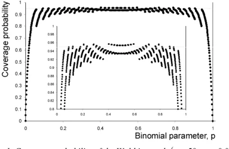
when the Wald interval (2) is used to generate the upper and lower

limits of the confidence interval produces Figure 1.

Figure 1. Coverage probability of the Wald interval,



n50,  0.05



In Figure 1 there are 1001 points (at 0, 0.001, 0.002, … 0.999, 1) of the unknown, but

constant value of the binomial parameter, p. 907 of these 1001 tests fail to meet the 95%

confidence limit (at the extremities, (7) is used in these results). Note that these results

are based on using z_ = 1.96. If z_ = 2 is used, then the chance of meeting the desired

confidence level will be slightly higher, with 799 of the 1001 tests failing to meet the

desired 95% confidence interval (note z_= 2 implies 95.47% confidence). If we follow

the advice of excluding ˆ 5np and n



1 pˆ



5 then 707 of the 1001 tests fail with z =

1.96 (if z_ = 2 is used, this reduces to 601 failures).For 90% desired confidence, there

are 801 failures in the 1001 tests. For 99% confidence there are 999 failures in the 1001 tests.

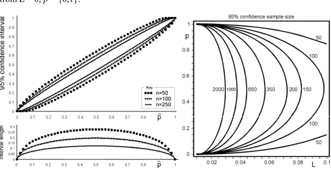
4.2. Length of the Wald interval

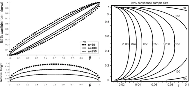
It is also interesting to investigate the length of the confidence interval. Figure 2 illustrates the upper and lower bound of the 95% Wald interval. It also highlights the length of the interval given by

ˆ ˆ

l pU pL

(9)

Note that for the Wald interval when L  pˆ



1 L



then  l 2L . However, when





ˆ 1

p L or ˆpL, then  _l 2L. This is a result of the boundary conditions in (2). It

can be seen in Figure 2 that the interval narrows as more samples are taken. Here we have

illustrated the case of n = 50, 100 and 250. Furthermore, the confidence interval is largest

at ˆ 0.5p and has zero length at ˆp= 0 and ˆp= 1. This is incorrect as it is known





1/ 0 if 0 ˆ / 2 n if L x p x n      _  and





1/ 1 / 2 if 0 ˆ 1 if n U x p x n          (7)

should be used at the extremities, Pires and Amano (2008). These are true the

Clopper-Pearson limits.

Figure 2 also contains a contour plot of the number of samples required to ensure 95%

confidence (according to (4)) as a function of the underlining binomial probability p, and

the interval half-width, L. It can be seen that the Wald interval (incorrectly) advises, for a

given interval half width, that the maximum number of samples required occurs when p =

0.5. The Wald interval also assumes (again incorrectly) that all the contours originate from L = 0, p = {0,1}.

Figure 2. Wald interval, its length and sample size requirement for 95% confidence 5. Evaluating the performance of a confidence interval for activity sampling

The review of the Wald interval has allowed us to introduce the terminology and the issues involved in binomial proportion confidence intervals. There are many such

intervals in the literature (see Pires and Amado, 2008). In order to select a confidence

interval for professional OM activity sampling we need some criteria to judge the field. First, and most importantly, the interval should actually achieve the desired confidence interval. That is, the coverage probability should be greater than the desired confidence level. Second, the length of the interval should be as small as possible, which probably means that excessive confidence should be avoided. Third, the confidence interval should work for different confidence levels. Forth, it should be easy to present and understand in a classroom setting.

(10)

We should also not need to make any a priori assumptions of the binomial probability p.

Whilst there are good performing conservative intervals (see Sterne (1954) for example)

that use a priori information, they are not suitable for activity sampling as the required

information is rarely available in a usable form. The procedure to determine the confidence interval is also rather complicated as the solution has no explicit form. Similar

arguments were made by Clopper and Pearson (1934), although Buck and Tanchoco

(1974) and Buck, Askin and Tanchoco (1983) have developed an activity sampling

procedure that does use a priori information.

There are also procedures available to modify confidence interval guidance. For example

Wang (2007) and Wang (2009) identifies the minimum coverage probability for a given sample and size and interval specification. He also provides a mechanism to determine the average coverage probability. Having determined the exact coverage probability (or the exact average coverage probability) one can then adjust (in an iterative approach) the

safety factor to achieve target confidence levels, see Agresti and Caffo (2000). We have

not pursued this approach either as this is a rather complex task. Rather we prefer to have a one-step calculation to the confidence interval calculation.

6. Alternative confidence intervals

This section reviews four other binomial confidence intervals. Three of these intervals are

approximate, one is exact. These four intervals where selected from Pires and Amado

(2008) as being described to possess (or nearly possess) the characteristics outlined in Section 5.

6.1. Agresti and Coull’s ‘Adjusted Wald’ interval

The first alternative confidence interval we will consider is based on a modification to the

Wald interval that was introduced by Agresti and Coull (1998), sometimes called the

Adjusted Wald interval. The expression for the boundaries of the interval with arbitrary

confidence levels is given by,







2





2



1 1

ˆU min ,1 and ˆL max ,0 ,

p z p z n z n z            _   _                    (8) where



2 ₂



2



1 x z_ n z_

     . Using (8) in (5) allows us to determine its coverage

(11)

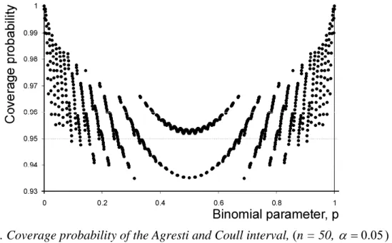
Figure 3. Coverage probability of the Agresti and Coull interval, (n = 50,  0.05)

For the record, 232 of 1000 tests fail to meet the 99% confidence target, 217 fail to meet the 95% target (above) and 305 fail the 90% target. While this is an improvement to the

coverage compared to the Wald interval, 20% to 30% of time, the desired level of

confidence is not actually achieved.

Figure 4 highlights the length of the Agresti and Coull interval for 95% confidence. Of note here is the fact that at the extremities of the probability,pˆ 

 

0,1 , the interval has a finite length. Also, the maximum and minimum operators in (8) are activated near the extremities. The sample size contours also exhibit more natural behaviour as they do not

all originate from the same point in the (L, p) plane. Note that in the contour plot, the

un-truncated behaviour (for L) was considered, as it was for Figure 2.

Figure 4. Agresti and Coull interval, its length and sample size requirements for 95% confidence

(12)

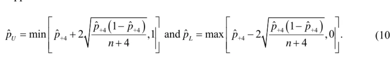
6.1.1. Agresti and Coull’s ‘Add 4’ interval

If you round the normal variant for 95% confidence from z_ 1.96 to z_ 2 and add

two successes and two failures to the sample population the Wald interval becomes

Agresti and Coull’s Add 4 interval. Starting with

4 2 ˆ 4 x p n   _ , (9)

the upper and lower intervals can be calculated with









+4 +4 +4 +4

+4 +4

ˆ 1 ˆ ˆ 1 ˆ

ˆ min ˆ 2 ,1 and ˆ max ˆ 2 ,0 .

4 4 U L p p p p p p p p n n  _   _                    (10)

Now only 76 of the 1000 tests fail to reach 95% coverage. Equation (10) is interesting as

it shows that if you do not collect any samples i.e. n = x = 0, then you can be confident

that 0 p 1, which is at least a logical result. It is possible to manipulate the un-truncated intervals in (10) to find a concise expression for the number of observations required to ensure p is within ˆpL,







2



2 4 4 ˆ ˆ 4 1 n p_ p_ L L . (11)

Figure 5. Coverage probability of the Add 4 interval,



n50,  0.05



Equation (12) adapts the Add 4 interval for arbitrary confidence levels. It produces 345 failures in the 1001 tests at the 90% confidence level, 211 failures at 95% and 351 failures at 99%.







1







1

+4 +4 +4 +4 +4 +4

ˆU ˆ ˆ 1 ˆ 4 and ˆL ˆ ˆ 1 ˆ 4

p  p z_ p p n  p  p z_ p p n  (12)

In summary, the Add 4 interval has a relatively simple closed form that is only slightly

more complex than the Wald interval. It can be manipulated for n, the number of samples

(13)

in a classroom setting, especially when students realise the implications of the Wald interval when p

 

0,1 .

6.2. Wilson Score interval

The Wilson Score interval is often quoted to be the statistician’s preferred choice for an approximation to the exact interval. The continuity corrected version of the Wilson score

interval is recommended by Pires and Amado (2008) and is given by,









2 2 1 1 2 1 if else ˆ ˆ 2 1 2 4 1 2 n n U x n x z z z x p p n z                   _  (13) and









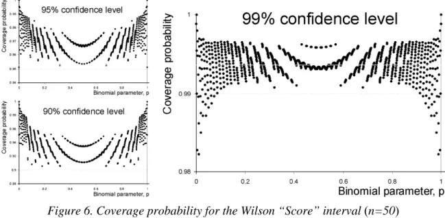
2 2 ₁ ₁ 2 0 if 0 else ˆ ˆ 2 1 2 4 1 . 2 n n L x x z z z x p p n z                   _  (14)

As we can see in Figure 6, the coverage probability for the 90% and 95% confidence levels is acheived. However, for the 99% confidence level the coverage probability is not met in 36 instances of the 1001 tests.

Figure 6. Coverage probability for the Wilson “Score” interval (n=50)

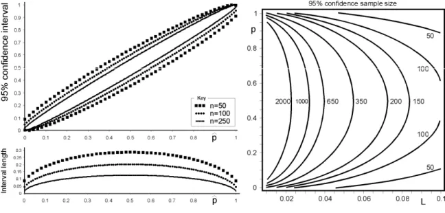
Figure 6 highlights the length of the Wilson Score interval for different sample sizes. It also shows that it deals with the extremities appropriately. It is possible to subtract (13)

from (14), set it equal to twice the interval half length (2L) and solve for n. It results in a

rather unwieldy solution to a forth order equation. However, it is easily plotted, see Figure 7. By closely comparing the sample size requirements the Wilson interval with the Agresti and Coull interval sample size requirements, we can see that the Wilson Score interval always requires more samples to be taken for a given probability and a given interval half width. This is perhaps the reason why the Wilson Score interval has such a high coverage probability.

(14)

Figure 7. The Wilson Score interval, its length and sample size requirements 6.3. The Arc Sin interval

The final approximate binomial confidence interval considered is the continuity corrected

Arc Sin interval discussed in Pires and Amado (2008). This is an interval based on the

approximate normal distribution interval after a variance stabilizing transformation. The Arc Sin interval is given by

7 2 8 3 1 4 2 1 if else ˆ sin arcsin 2 U x n p x z n n     _ _  _  _ _  _ _ _ _    (15) and 1 2 8 3 1 4 2 0 if 0 else ˆ sin arcsin . 2 L x p x z n n     _ _  _  _ _  _ _ _ _    (16)

(15)

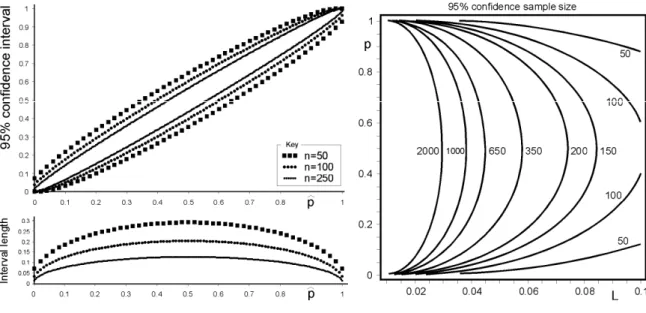
The Arc Sin interval actually achieves 90% and 95% coverage, but fails to meet 6 of the 1001 tests at 99% coverage probability. This is an improvement upon the Wilson Score interval, especially as 4 of the 6 failures at 99% coverage occur very close to the extreme values of the binomial probability. However, the interval is very large, see Figure 9.

Figure 9. The 95% Arc Sin confidence interval, its length and sample size requirements 6.4. The Clopper-Pearson interval

An exact solution of the confidence interval is one that always reaches the desired coverage probability. The original approach to this solution is based on finding the real

root within the valid probability range of a polynomial of an order equal to n1, Clopper

and Pearson (1934). Specifically, the upper boundary of the Clopper-Pearson confidence interval is given by the real solution in the range [0..1] to





0 ˆ 1 ˆ . 2 x n k k U U k n p p k      _ _    



(17)

Similarly the lower boundary is given by the real solution, in the range [0..1], to





ˆ 1 ˆ 2 n n k k L L k x n p p k      _ _    



. (18)

This form of the Clopper-Pearson interval is rather hard to deal with when n becomes

large. However, the Clopper-Pearson interval can also be expressed in a more

manageable form that uses the Beta distribution (see Newcombe (1998) and Pires and

Amado (2008)) as follows,

 

1/ 2 1 2 1 if 0 ˆ 1 if else 1 , 1, n U x p x n B x n x        _   _ _ _ _ _    and

 

₂ 1/ 1 2 0 if 0 ˆ if else , , 1 n L x p x n B x n x       _   _ _{ } _     (19) where 1





1 2 , ,

B    is the  percentile of the Beta



 ₁, ₂



distribution. This form of the Clopper-Pearson interval is easy to handle with modern statistical and mathematical

(16)





ˆU BETAINV 1 2, 1, p   x nx (20) and





ˆL BETAINV 2, , 1 p   x n x . (21)

Johnston, Kemp and Kotz (2005) provide a comprehensive list of references to tables of confidence intervals. They also note the link between the Clopper-Pearson interval and the F distribution and provide the following guidance for the upper limit of the confidence interval, 1 2 1 2 1 , ,1 2 2 1 , ,1 2 ˆ v v , U v v v F p v v F       (22)

where v12

 

x1 and v2 2



nx



. The lower limit of the interval is

1 2 1 2 1 , , 2 2 1 , , 2 ˆ v v , L v v v F p v v F     (23)

with v₁2x and v₂ 2



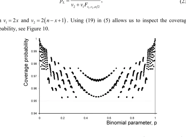
n x 1



. Using (19) in (5) allows us to inspect the coverage probability, see Figure 10.

Figure 10. Coverage probability of the Clopper-Pearson interval,



n50,  0.05



Figure 10 confirms that for the Clopper-Pearson interval when n50 and  0.05 the

coverage probability is always greater than the desired confidence level. However, because of the discrete nature of the binomial distribution it can often be rather conservative, especially in the extremities of the binomial probability. The confidence interval and its length is portrayed in Figure 11. Here we can see that the interval is largest near ˆp= 0.5, is symmetrical about ˆp= 0.5, and has a finite length at pˆ 

 

0,1 .

(17)

Figure 11. The 95% Clopper-Pearson confidence interval, its length and sample size requirements

The inverse problem where we solve the Clopper-Pearson equations for n, was studied by

Johnston, Kemp and Kotz (2005). They highlight that (24) and (25) can be solved to yield

an upper and lower limit on n, n_U and n_L , such that p is within ˆpL with



1 _



100% confidence;



 



ˆ 0 ˆ 1 ˆ 2 U U n p k n k U k n p L p L k           



, (24)



 



ˆ ˆ 1 ˆ 2 L L L n k n k L k n p n p L p L k           



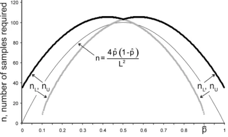
. (25)

Solving (24) and (25) plotting nU and nL for different values of p when the interval half

length, L = 0.1 and  0.05 yields Figure 12. Here we can see the two curves for n_U and

L

n . Obviously we will need to pick the largest n for a particular observed probability, ˆp.

Hence, the parts of the curves that are plotted in grey become redundant. We can also see that solutions nL < L and nU  1 L do not exist as ˆp cannot be less than zero or greater than unity. Interestingly, the maximum number of observations required does not occur

when ˆp_{= 0.5 (which was advocated by all of the previously considered intervals - see}

the solid line in Figure 12 for the Wald interval). Rather the maximum observations occur

near 1

2

ˆ L

  (but not precisely at 1

2

ˆ

p L, due to the discrete nature of the binomial

distribution). The nature of the two solutions to (24) explains why Figure 11 does not

have contours that are maximal in L at p0.5. Figure 12 also highlights that the Wald

interval never takes enough observations to ensure that both sides of the interval have less

(18)

Figure 12. Sample size required for L = 0.1, 95% confidence

Defining L as the maximum L in the level sets of the contour plot in Figure 11 allows us

to obtain an upper bound of the number of samples required to achieve a desired interval

half-width. A visualisation of the relationship between L and n is given in Figure 13.

Here we can see that the maximum interval half-width reduces as more samples are taken,

but there is a law of diminishing returns with large samples sizes.

Figure 13. Minimum sample size requirements to ensure L<L+, 95% confidence

7. Recommendation of a confidence interval for activity sampling

Table 2 summaries the test results from Sections 4 and 6. If you require the most simple

interval possible for 95% confidence, then you could (continue to) use the simplified Wald interval. This does not guarantee the coverage required (about 80% of the time) and

assumes the user lacks the capability to exploit a more sophisticated approach. A

literature review demonstrated that this approach is almost exclusively advocated by the OM field.

(19)

A more meaningful interval for 95% confidence is the Add 4 interval. This greatly improves the coverage probability of the Wald interval and also has a simple closed form solution for the number of samples required to be within a desired tolerance.

To be sure that the coverage probability was achieved (at least for 90% and 95%, and almost sure for 99% confidence) in situations where a closed form expression is required, the continuity corrected Wilson Score interval is recommended. Whilst it is possible to manipulate the interval for n, given a target interval length, it is rather complex for

classroom use.

If one is willing to drop the requirement for a closed form, the Arc Sin interval ensures the coverage probability is assured for both 90% and 95% confidence. However, for 99% confidence the interval does not achieve the required coverage at the extremities (and for a small number of points in the middle). It is possible to find the sin and arcsin functions on most good handheld calculators, hence it may be relevant for practising industrial engineers.

Finally, if you must ensure the coverage probability is met and have access to the Clopper-Pearson tables given in Appendix B (or access to the inverse beta distribution in Microsoft Excel) then the Clopper-Pearson interval is recommended. This is the only

interval that guarantees the desired coverage probability for all values of _ and p.

Interval 90% Confidence level desired 95% 99% Notes

Wald 801 fails _{(799 fails if}907 fails

z=2) 999 fails Most simple closed form

Agresti & Coull’s

‘Adjusted Wald’ 305 fails 217 fails 232 fails Improved performance over Wald

Agresti & Coull’s

‘Add 4’ 345 fails (76 fails if 211 z=2) 351 fails

Nice simple closed form for interval and for sample size

requirements

Wilson Score 0 fails 0 fails 36 fails Complex closed form

Arc Sin 0 fails 0 fails 6 fails No closed form, but easily done on _{a scientific calculator.}

Clopper-Pearson 0 fails 0 fails 0 fails

No closed form, but amenable in Excel. Easily presented in tabular

form. Sample size requirements possible

Table 2. Summary results from 1001 confidence interval trials for activity sampling

Notwithstanding the arguments above, let’s now investigate the contour plots in Figures 2, 4, 7, 9 and 11 again. Overlaying them all into one single plot as in Figure 14, it is possible to see when one interval dominates the other in terms of reducing the interval to a specific half-width with a particular sample size. Note we are ignoring whether the coverage probability actually meets the desired confidence level here. It can be seen that the Agresti and Coull interval generally dominates all of the other intervals. That is, it requires fewer samples to meet its specific half-width. The Wilson interval generally dominates all other intervals, except the Agresti and Coull interval. This can be regarded as good performance as the Wilson Score interval is almost exact. The Arc Sin interval generally dominates the Clopper-Pearson interval. Despite this, it is recommended that the standard operations management procedure is updated to include the Clopper-Pearson interval.

(20)

Figure 14. Comparison of the five confidence intervals by sample size requirements

8. Activity sampling procedure using the Clopper-Pearson interval

A procedure to exploit the Clopper-Pearson interval for activity sampling will now be described. Appendix A provides a blank data collection form. The Clopper-Pearson confidence interval requires either; the solution of pair of high order equations (equations (17) and (18)); access to Microsoft Excel to enumerate (20) or specialist statistical software to realise (22) and (23)); or access to Clopper-Pearson confidence interval tables. Appendix B provides Clopper-Pearson confidence intervals that fit the data collection

forms for the case of n = 50, 100 and 150. Appendix C gives the maximum of the

solution to (24) and (25), rounded up to the nearest integer, for the required number of

samples n to be within a desired interval half-width for 90%, 95% and 99% confidence

for different values of the estimated binomial parameter, ˆp.

The following step-by-step guide highlights how to use these tools.

Step 1. Determine how much confidence you need to assign to your results. From this,

determine the value of _.

Step 2. Determine an acceptable confidence interval half length (L) for the purposes of

your study. Note. Steps 1 and 2 should be done in consultation with the “customer” of the activity sampling exercise.

Step 3. Explain the purpose of the activity sampling to the subjects of the exercise, (the

workers, customers, operators etc). Obtain an initial impression of range of activities being undertaken by the workers, their duration and their frequency. Make a note of the working time, breaks and any data collection issues present.

Step 4. Modify the activity sampling data collection form in Appendix A for your

situation. Name each of the activities the subject (worker, customer, machine etc) undertakes in the columns A to J. If there are not enough columns then you need to develop your own forms. Specify when the observations are to be taken

(21)

distributed random numbers appropriately scaled to fit your scenario. Make sure the study is long enough to capture the range of activities that are undertaken.

Step 5. Collect the activity sample. First collect 50 samples (a page worth). Total up the

observations for each activity and calculate the upper and lower limits of confidence interval, using the table of Clopper-Pearson confidence intervals in Appendix B. Decide if the confidence interval meets the needs of the study. If it is not then use Appendix C to determine how many samples should be taken in

order to reduce the interval half-width (L) to an acceptable level.

Step 6. If the confidence interval half length (L) is too large for your purpose, collect

another 50 samples using the data collection form and re-calculate the length of the interval.

Step 7. Repeat steps 5 and 6 until you are satisfied with the accuracy of the confidence

interval for each of the activities.

9. Teaching activity sampling with the new Clopper-Pearson interval

This new activity sampling procedure has been taught to over 2000 students over the last 5 years in Undergraduate, MSc, MBA and Executive courses in the U. S. and the U. K. Only the Clopper-Pearson interval is discussed. No detail on other alternative intervals needs to be given. The data collection forms and tables of intervals and sample sizes are no more difficult to use than a standard normal table. Students often struggle with the

difference between and selection of appropriate accuracy

 

L and confidence

 

 , so it

is worthwhile spending some time on this matter. However, on balance, the new Clopper-Pearson approach is actually easier to teach as students often find the circular reference to

p in the Wald interval formula difficult. It is also easy to break-out of a presentation to

illustrate the Inverse Beta function in Microsoft Excel.

A worked example (activity sampling my 2 year old daughter), a class exercise of activity sampling a secretary’s duties and case study at Sam’s Tailor in Hong Kong is used. These

teaching materials are available upon request from the author. Sohal and Oakland (1990)

also offer some advice on an engaging method to teach activity sampling that could also be adopted for use within this Clopper-Pearson activity sampling procedure.

10. Concluding remarks

The standard operations management textbook treatment of activity sampling has been evaluated. It was found that the Wald interval is almost exclusively used to assign confidence to the results. A review of modern statistical knowledge on binomial proportion confidence intervals revealed that the statisticians have serious concerns with the adequacy of this interval and have developed a range of more sophisticated approximations. There is even an exact solution to the problem.

These modern confidence intervals have been reviewed and analysed for the purpose of activity sampling. The Clopper-Pearson interval was found to be the only interval that actually achieves the desired confidence interval for any desired coverage probability that

does not use a-priori information. The Clopper-Pearson interval has an explicit solution,

but sadly has no closed form. However, given that Microsoft Excel has an Inverse Beta Distribution function built-in, the Clopper-Pearson interval can be easily determined.

(22)

Two look-up tables for the interval and the sample size requirements have been developed for classroom use.

A new activity sampling procedure was developed that can be used without advanced statistical knowledge to gather information about many operations management scenarios. The interval obtained now economically achieves the desired coverage. The existing activity sampling procedure in many OM textbooks cannot guarantee this.

References

Adam, E.E. and Ebert, R.J., (1992), Production and Operations Management: Concepts,

Models and Behaviour. Prentice-Hall Inc, New Jersey, USA, 314-315.

Agresti, A., and Coull, B., (1998), “Approximate is better than 'exact' for interval

estimation of binomial proportions”, The American Statistician, 52 (2), 119-126.

Agresti, A. and Caffo, B., (2000), “Simple and effective confidence intervals for

proportion and differences of proportions result from adding two successes and two

failures”, The American Statistician,54 (4), 280-288.

Anderson, D.R., Sweeney, D.J., Williams, T.A., Freeman, J. and Shoesmith, E., (2007),

Statistics for Business and Economics. Thomson, London, UK, 273-276.

Barnes, D., (2008), Operations Management: An International Perspective. Thomson

Learning, London, UK, 345.

Bicheno, J. and Holweg, M., (2009), The Lean Toolbox: The Essential Guide to Lean

Transformation. Picsie Books, Buckingham, UK, 130-131.

Bicheno, J., (2008), The Lean Toolbox for Service Systems. Picsie Books, Buckingham,

UK, 271-272.

Blyth, C.R. and Still, H.A., (1983), “Binomial confidence intervals”, Journal of the

American Statistical Association, 78 (381), 108-116.

Brisley, C.L., (2001), “Work sampling and group timing technique”, Chapter 17.3 in

Zandin, K.B., (2001), Maynard’s Industrial Engineering Handbook. Fifth Edition,

McGraw-Hill, New York, USA, 17.47-17.64.

British Standard 3138, (1992), “Glossary of terms used in management services”, p12. Brown, L.D., Cai, T.T., and DasGupta, A., (2001), “Interval Estimation for a Binomial

Proportion”, Statistical Science, 16 (2), 101-117.

Buchholz, B., Paquet, V., Punnett, L., Lee, D. and Moir, S., (1996), “PATH: A work sampling-based approach to ergonomic job analysis for construction and other

non-repetitive work”, Applied Ergonomics, 27 (3), 177-187.

Buck, J.R. and Tanchoco, J.M.A., (1974), “Sequential Bayesian work sampling”, AIIE

Transactions, 6 (4), 318-326.

Buck, J.R., Askin, R.G. and Tanchoco, J.M.A., (1983), “Advances in sequential Bayesian

work sampling”, IIE Transactions, 15 (1), 19-30.

Chase, R.B. and Aquilano N.J., (1992), Production and Operations Management. Irwin

In., Boston, USA, 518-524.

Chen, J.-G., Peacock, J.B. and Schlegel, R.E., (1989), “An observational technique for

physical work stress analysis”, International Journal of Industrial Ergonomics, 3

(3), 167-176.

Clopper, C. and Pearson, S., (1934), “The use of confidence or fiducial limits illustrated

in the case of the binomial”. Biometrika, 26 (4), 404-413.

Curwin, J. and Slater, R., (1990), Quantitative Methods for Business Decisions. Chapman

and Hall, London, UK, 198-201.

Davis, M.M. and Heineke, J., (2005), Operations Management: Integrating

Manufacturing and Services. McGraw- Hill Irwin, New York, 257-261.

(23)

Farrell, P.J., Kusy, M., Tomberlin, T.J. and Thomas, R., (2009), “A hybrid methodology

for measuring unit costs in multibranch institutions”, Canadian Journal of

Administrative Sciences, 14 (2), 188 – 194.

Finch, B.J., (2008), Operations Now: Supply Chain Profitability and Performance.

McGraw-Hill Irwin, Boston, USA, 757-758.

Finkler, S.A., Knickerman, J.R., Hendrickson, G., Lipkin, M. and Thompson, W.G., (1993), “A comparison of work sampling and time-and-motion techniques for

studies in health services research”, Health Services Research, 28 (5), 577-597.

Foley, W.J., (1999), “National nursing home restraint minimization project”, Internal Report, Rensselaer Polytechnic Institute, Troy, New York, USA.

Greasely, A., (2009), Operations Management. John Wiley, Chichester, UK, 244-246.

Gunesoglu, S. and Meric, B., (2006), “The analysis of personal and delay allowances using work sampling technique in the sewing room of a clothing manufacturer”,

International Journal of Clothing Science and Technology, 19 (2), 145-150.

Heinze, K.G.R., (1984), “Performance measures by means of activity sampling”,

Transactions of the American Association of Cost Engineers, D (4), 1-8.

Heizer, J. and Render, B., (2014), Operations Management. Pearson, New Jersey, USA,

435-438.

Hill, T., (1983), Production and Operations Management. Prentice Hall, London,

246-248,

Hill, T., (2000), Operations Management: Strategic Context and Managerial Analysis.

Palgrave, Basingstoke, UK, 480-481.

International Labour Office, (1974), Introduction to Work Study: Revised Edition. ILO

Geneva, Switzerland, 369-377.

Jacobs, F.B., Chase, R.B. and Aquilano, N.J., (2009), Operations and Supply

Management. McGraw-Hill Irwin, Boston, USA, 194-200.

Johnson, N.L., Kemp, A.W., Kotz, S., (2005), Univariate Discrete Distributions. John

Wiley and Sons, New Jersey, USA.

Kaming, P.F., Olomolaiye, P.O., Holt, G.D. and Harris, F.C., (1997), “Factors

influencing craftsmen’s productivity in Indonesia”, International Journal of Project

Management, 15 (1), 21-30.

Kelly, J., (1964), “The study of executive behaviour by activity sampling”, Human

Relations, 17 (3), 277-287.

Khanna, R.B., (2015), Production and Operations Management, PHI Learning, Delhi,

pp137-139.

Krajewski, L., Ritzman, L. and Malhotra, M., (2013), Operations Management Processes

and Value Streams. Pearson Prentice Hall, New Jersey, USA, 148.

Lee, S.M. and Schniederjans, M.J., (1994), Operations Management. Houghton Mifflin,

Boston, USA, 709-712.

Liou, F.-S. and Borcherding, J.D., (1986), “Work sampling can predict unit rate

productivity”, Journal of Construction Engineering and Management, 112 (1),

90-103.

Lockyer, K., (1983), Production Management. Pitman, London, UK, 196-200.

Lockyer, K., Muhlemann, A. and Oakland, J., (1988), Production and Operations

Management. Pitman Publishing, London, UK, 250-252.

Meredith, J.R., (1992), The Management of Operations. John Wiley and Sons, New York,

USA, 710-711.

Naylor, J., (1996), Operations Management, Pitman Publishing, London, 170.

Newcombe, R.G., (1998), “Two-sided confidence intervals for the single proportion:

Comparison of seven methods”, Statistics in Medicine, 17 (8), 857-872.

Noori, H. and Radford, R., (1995), Production and Operation Management: Total

(24)

Pelletier, D. and Duffield, C., (2003), “Work sampling: Valuable methodology to define

nursing practice patterns”, Nursing and Health Sciences, 5 (1), 31-38.

Pires, A.M. and Amado, C., (2008), “Interval estimators for a binomial proportion:

Comparison of twenty methods”, Revstat – Statistical Journal, 6 (2), 165-197.

Reid, R.D. and Sanders, N.R., (2002), “Operations Management”, John Wiley, New

York, USA, 337-338.

Rosenkrantz, W.A., (2009), Introduction to Probability and Statistics for Science,

engineering and finance. CRC Press, Boca Raton, USA, 307-309.

Russell, R.S. and Taylor, B.W., (2009), Operations Management Along the Supply Chain.

John Wiley, Singapore, pp346-348.

Rutter, R., (1994), “Work sampling: As a win-win management tool”, Industrial

Engineering, 26 Feburary, 30-31.

Schonberger, R.J. and Knod, E.M., (1988), Operations Management: Serving the

Customer. Business Publications, Plano, USA, 666-670.

Silver, M., (1997), Business Statistics. McGraw-Hill, London, UK, 191-192.

Slack, N., Brandon-Jones, A. and Johnston, R., (2013), Operations Management. FT

Prentice Hall, Harlow, UK, 268.

Sohal, A.S. and Oakland, J.S., (1990), “Teaching production and operations management

through participative methods”, Production and Inventory Management Journal, 31

(3), 30-34.

Sterne, T.E., (1954), “Some remarks on confidence or fiducial limits”, Biometrika, 41

(1-2), 275-278.

Stevenson, W.J., (2012), Operations Management: Theory and Practice. McGraw-Hill,

Irwin, 308-313.

Thomas, H.R., (1991), “Labour productivity and work sampling: The bottom line”,

Journal of Construction Engineering and Management, 117 (3), 423-444.

Tippett, L.H.C., (1935), “A snap-reading method of making time studies of machines and

operatives in factory surveys”, Journal of the Textile Institute Transactions, 26 (2),

51-55 & 75.

Tsai, W.-H., (1996), “A technical note on using work sampling to estimate the effort on

activities under activity based costing”, International Journal of Production

Economics, 43 (1), 11-16.

Wald, A. and Wolfowitz, J., (1939), “Confidence limits for continuous distribution

functions”, Annals of Mathematical Statistics, 10 (2), 105-118.

Wang, H., (2007), “Exact confidence coefficients of confidence intervals for a binomial

proportion”, Statistica Sinica,17 (1), 361-368.

Wang, H., (2009), “Exact average coverage probabilities and confidence coefficients of

confidence intervals for discrete distributions”, Statistics and Computing, 19 (2),

139-148.

Waters, D., (2002), Operations Management: Producing Goods and Services. FT

Prentice Hall, Harlow, UK, 500.

Weiss, H.J. and Gershon, M.E., (1989), Production and Operations Management. Allyon

and Bacon, Boston, USA, 419-423.

Whitmore, D.A., (1987), Work Measurement. Heinemann, London, UK, pp118-127.

Wild, R., (1995), Production and Operations Management: Text and Cases. Cassell

Education, London, UK, 188-191.

Williams, H., Harris, R. and Turner-Stokes, L., (2009), “Work sampling: A quantitative

analysis of nursing activity in a neuro-rehabilitation setting”, Journal of Advanced

(25)

Appendix A: Activity sampling data collection form

Title:

Confidence,____% ,_____ L,____ Date:

Purpose: Completed by:

Page ___ of ____ Ob servatio n Number Uniformly distributed random numbers Intervals driven by random numbers? Y / N Activity A B C D E F G H I J Time of observation 1 98837 67136 2 35311 82655 3 18581 30998 4 81781 03347 5 38285 66912 6 24689 72155 7 93492 29368 8 10281 25221 9 95991 99716 10 57579 12203 11 12468 46011 12 72758 75741 13 86051 48890 14 31430 48040 15 96616 99230 16 92753 37184 17 55585 79446 18 27108 38086 19 53103 45868 20 47128 69377 21 67866 53793 22 35611 99785 23 58725 87497 24 67091 07571 25 28792 56073 26 94790 89294 27 54599 55184 28 44346 65363 29 45804 30298 30 50371 55805 31 53271 59910 32 25086 73884 33 98339 14198 34 08591 41964 35 94737 28459 36 42328 97773 37 25380 31213 38 87258 46559 39 83390 54356 40 94856 27832 41 77092 40946 42 76977 34774 43 15537 11515 44 15033 90458 45 63078 91904 46 13037 90690 47 62328 62666 48 51910 39671 49 37489 05840 50 01641 53158

Running count from any previous samples (n = ) Total sum of observations, x

Observed probability, ˆ  x n

p

Lower confidence interval, pˆ_L (App. B) Upper confidence interval, pˆ_U (App. B) Sample size required based on L (App. C)

(26)

Appendix B: Table of Clopper-Pearson confidence intervals

n=50 ˆpLypÛ 1 y pÛypˆL 1 y n=150 ˆpLypÛ 1 y pÛypˆL 1 y x 99% 95% 90% 90% 95% 99% x 99% 95% 90% 90% 95% 99% 0 (50) y=0 0 0 0.058155079 0.071121736 0.100545083 0 (150) y=0 0 0 0.019773438 0.024292597 0.03470557 1 (49) 0.000100246 0.000506228 0.00102534 0.091398131 0.106469546 0.139404125 1 (149) 3.34164E-05 0.000168771 0.000341897 0.031233817 0.036583168 0.048485953 2 (48) 0.002088725 0.004881433 0.00715372 0.120614155 0.137137626 0.17250176 2 (148) 0.000692036 0.001618827 0.002374192 0.04137497 0.047333019 0.060345774 3 (47) 0.006872485 0.012548588 0.016551859 0.147837176 0.165481947 0.202706269 3 (147) 0.002265007 0.004143625 0.00547293 0.050877068 0.057334222 0.071262464 4 (46) 0.013768445 0.022227964 0.027787668 0.173791158 0.192342784 0.23105085 4 (146) 0.004516558 0.007312546 0.009158928 0.05998104 0.066867877 0.081586214 5 (45) 0.022217815 0.033275094 0.04023659 0.198833003 0.218135366 0.258049729 5 (145) 0.007257229 0.010910186 0.013224408 0.068805184 0.076072323 0.091490565 6 (44) 0.031862914 0.045335321 0.053571403 0.22316999 0.243101317 0.284003704 6 (144) 0.010366487 0.014818521 0.017560962 0.077417997 0.085027815 0.101076706 7 (43) 0.042468787 0.0581917 0.067596699 0.246935202 0.267396002 0.309106966 7 (143) 0.013765426 0.01896557 0.02210405 0.08586338 0.093785865 0.110409837 8 (42) 0.053873602 0.071700767 0.082185062 0.270220078 0.291126307 0.333493522 8 (142) 0.017399794 0.02330381 0.026811658 0.094171482 0.102381896 0.119534935 9 (41) 0.065961072 0.085762078 0.097248095 0.293090581 0.314369411 0.357260386 9 (141) 0.021230608 0.027799978 0.031654647 0.102364084 0.11084152 0.128484599 10 (40) 0.078644691 0.100302237 0.112721613 0.315596061 0.337183108 0.380480351 10 (140) 0.025228817 0.032429728 0.036611832 0.110457532 0.119183977 0.137283372 11 (39) 0.091858295 0.115265826 0.128557379 0.337774485 0.359611889 0.403209554 11 (139) 0.029372118 0.037174615 0.041667235 0.118464471 0.127424162 0.145950285 12 (38) 0.105550132 0.130609916 0.144718155 0.359655697 0.381690748 0.425492219 12 (138) 0.033642958 0.042020265 0.046808451 0.126394927 0.13557389 0.154500458 13 (37) 0.119679002 0.146300584 0.161174597 0.381263556 0.403447679 0.447363763 13 (137) 0.038027232 0.04695522 0.052025622 0.134257008 0.143642723 0.162946142 14 (36) 0.134211639 0.162310601 0.177903198 0.402617382 0.424905357 0.468852912 14 (136) 0.04251341 0.051970172 0.057310755 0.142057385 0.151638531 0.171297434 15 (35) 0.149120897 0.178617846 0.194884897 0.423732967 0.446082326 0.48998318 15 (135) 0.047091922 0.057057435 0.062657265 0.149801626 0.159567885 0.17956277 16 (34) 0.164384449 0.195204195 0.212104098 0.444623296 0.46699384 0.510773932 16 (134) 0.051754723 0.062210574 0.068059646 0.157494434 0.167436339 0.18774929 17 (33) 0.179983844 0.212054713 0.229547962 0.465299081 0.487652488 0.531241159 17 (133) 0.056494972 0.06742414 0.073513243 0.165139829 0.175248639 0.195863098 18 (32) 0.195903809 0.229157067 0.247205894 0.485769151 0.508068648 0.551398063 18 (132) 0.061306798 0.072693467 0.079014074 0.172741273 0.183008877 0.203909461 19 (31) 0.21213172 0.246501078 0.265069158 0.506040748 0.528250837 0.571255486 19 (131) 0.066185114 0.078014525 0.084558705 0.18030178 0.190720614 0.211892966 20 (30) 0.228657206 0.264078395 0.283130591 0.526119749 0.548205972 0.590822246 20 (130) 0.071125481 0.083383807 0.090144145 0.187823988 0.198386968 0.219817631 21 (29) 0.245471848 0.281882241 0.301384377 0.546010837 0.567939565 0.610105383 21 (129) 0.076123996 0.088798232 0.095767775 0.195310223 0.206010689 0.227687004 22 (28) 0.262568945 0.299907221 0.319825889 0.565717627 0.587455877 0.629110348 22 (128) 0.081177208 0.094255085 0.101427285 0.20276255 0.213594219 0.235504232 23 (27) 0.279943342 0.318149179 0.338451559 0.585242759 0.606758024 0.647841147 23 (127) 0.086282047 0.099751951 0.107120622 0.210182807 0.221139733 0.243272126 24 (26) 0.297591302 0.336605092 0.35725879 0.604587965 0.625848055 0.666300434 24 (126) 0.09143577 0.105286678 0.112845957 0.217572646 0.228649184 0.250993204 25 0.315510421 0.355272997 0.376245891 0.623754109 0.644727003 0.684489579 25 (125) 0.096635913 0.110857332 0.118601649 0.22493355 0.236124327 0.258669737 26 (124) 0.101880252 0.116462173 0.12438622 0.232266861 0.24356675 0.266303776 n=100 ˆpLypÛ 1 y pÛypˆL 1 y 27 (123) 0.107166776 0.122099628 0.130198336 0.239573797 0.250977895 0.273897184 x 99% 95% 90% 90% 95% 99% 28 (122) 0.112493654 0.127768266 0.136036784 0.246855466 0.258359073 0.281451656 0 (100) y=0 0 0 0.02951305 0.036216693 0.05160403 29 (121) 0.117859222 0.133466786 0.14190046 0.25411288 0.265711481 0.288968742 1 (99) 5.01242E-05 0.000253146 0.000512801 0.046559811 0.054459385 0.071957682 30 (120) 0.123261954 0.139193999 0.147788357 0.261346965 0.273036218 0.296449862 2 (98) 0.001039619 0.002431337 0.003565153 0.0616192 0.070383932 0.089430673 31 (119) 0.128700453 0.144948816 0.153699551 0.268558571 0.280334289 0.303896318 3 (97) 0.00340707 0.006229972 0.008225829 0.075710794 0.085176053 0.105481254 32 (118) 0.134173435 0.150730237 0.159633196 0.275748483 0.287606623 0.311309311 4 (96) 0.006801694 0.011004494 0.013776612 0.08919625 0.099257157 0.120632699 33 (117) 0.139679717 0.156537338 0.16558851 0.282917421 0.294854074 0.318689949 5 (95) 0.010940334 0.016431879 0.019905564 0.102253378 0.112834911 0.135144683 34 (116) 0.145218205 0.162369272 0.171564774 0.290066054 0.302077433 0.326039255 6 (94) 0.015642513 0.022334886 0.026449713 0.114985256 0.126029935 0.149168804 35 (115) 0.15078789 0.168225251 0.177561322 0.297195 0.309277432 0.333358178 7 (93) 0.02078993 0.028605289 0.033311916 0.127458016 0.138919728 0.162802856 36 (114) 0.156387835 0.174104547 0.183577538 0.304304832 0.316454751 0.340647598 8 (92) 0.026301152 0.035171563 0.040428871 0.139717119 0.151557636 0.176114355 37 (113) 0.16201717 0.180006485 0.189612851 0.311396082 0.32361002 0.347908333 9 (91) 0.032117617 0.041983596 0.047756636 0.151795429 0.163982255 0.18915228 38 (112) 0.167675086 0.185930437 0.195666728 0.318469248 0.330743828 0.355141143 10 (90) 0.038195653 0.049004689 0.055263238 0.163717623 0.176222598 0.201953521 39 (111) 0.173360831 0.191875818 0.201738676 0.325524789 0.337856721 0.362346739 11 (89) 0.044501714 0.05620702 0.06292455 0.175502803 0.188301132 0.214546698 40 (110) 0.179073703 0.197842083 0.207828234 0.332563138 0.344949209 0.369525782 12 (88) 0.051009388 0.063568903 0.070721838 0.18716611 0.200235684 0.226954552 41 (109) 0.184813047 0.203828725 0.213934972 0.339584697 0.352021771 0.37667889 13 (87) 0.057697454 0.071073046 0.078640204 0.198719793 0.212040677 0.239195508 42 (108) 0.190578251 0.209835269 0.220058489 0.346589841 0.35907485 0.383806642 14 (86) 0.064548563 0.078705405 0.086667578 0.210173925 0.223727981 0.2512847