Learning Code Transformations via Neural Machine Translation

(1)

W&M ScholarWorks

Dissertations, Theses, and Masters Projects Theses, Dissertations, & Master Projects 2019

Michele Tufano

William & Mary - Arts & Sciences, tufanomichele89@gmail.com

Follow this and additional works at: https://scholarworks.wm.edu/etd

Part of the Computer Sciences Commons

Recommended Citation Recommended Citation

Tufano, Michele, "Learning Code Transformations via Neural Machine Translation" (2019). Dissertations, Theses, and Masters Projects. Paper 1563899006.

http://dx.doi.org/10.21220/s2-1z1j-d577

This Dissertation is brought to you for free and open access by the Theses, Dissertations, & Master Projects at W&M ScholarWorks. It has been accepted for inclusion in Dissertations, Theses, and Masters Projects by an authorized administrator of W&M ScholarWorks. For more information, please contact scholarworks@wm.edu.

(2)

Learning Code Transformations via Neural Machine Translation

Michele Tufano Avellino, Italy

Bachelor in Computer Science, University of Salerno, 2012 Master in Computer Science, University of Salerno, 2014

A Dissertation presented to the Graduate Faculty

of The College of William & Mary in Candidacy for the Degree of Doctor of Philosophy

Department of Computer Science

College of William & Mary April 2019

(3)

(4)

(5)

ABSTRACT

Source code evolves – inevitably – to remain useful, secure, correct, readable, and

efficient. Developers perform software evolution and maintenance activities by

transforming existing source code via corrective, adaptive, perfective, and

preventive changes. These code changes are usually managed and stored by a variety of tools and infrastructures such as version control, issue trackers, and code review systems. Software evolution and maintenance researchers have been mining these code archives in order to distill useful insights regarding the nature of

developers’ activities. One of the long-lasting goals of software engineering research is to better support and automate different types of code changes

performed by developers. In this thesis we depart from classic manually crafted rule- or heuristic-based approaches, and propose a novel technique to learn code

transformations by leveraging the vast amount of publicly available code changes performed by developers. We rely on Deep Learning, and in particular on Neural Machine Translation (NMT), to train models able to learn code change patterns and apply them to novel, unseen, source code.

First, we tackle the problem of generating source code mutants for Mutation Testing. In contrast to classic approaches, which rely on handcrafted mutation operators, we propose to automatically learn how to mutate source code by observing real faults. We mine millions of bug fixing commits from GitHub, and then process and abstract this source code. This data is used to train and evaluate an NMT model to translate fixed code into buggy code (i.e., the mutated code).

In the second project, we rely on the same dataset of bug-fixes to learn code transformations for the purpose of Automated Program Repair (APR). This represents one of the most challenging research problem in Software Engineering, whose goal is to automatically fix bugs without developers’ intervention. We train a model to translate buggy code into fixed code (i.e., learning patches) and, in

conjunction with beam search, generate many different potential patches for a given buggy method. In our empirical investigation we found that such a model is able to fix thousands of unique buggy methods in the wild. Finally, in our third project we push our novel technique to the limits by enlarging the scope to consider not only bug-fixing activities, but any type of meaningful code changes performed by developers. We focus on accepted and merged code changes that have undergone a Pull Request (PR) process. We quantitatively and qualitatively investigate the code transformations learned by the model to build a taxonomy. The taxonomy shows that NMT can replicate a wide variety of meaningful code changes, especially refactorings and bug-fixing activities.

In this dissertation we illustrate and evaluate the proposed techniques, which represent a significant departure from earlier approaches in the literature. The promising results corroborate the potential applicability of learning techniques, such as NMT, to a variety of Software Engineering tasks.

(6)

ACKNOWLEDGMENTS

This Dissertation would not have been possible without the advice and support of several people. First, I would like to thank my advisor Dr. Denys Poshyvanyk. He has been an exceptional mentor and friend to me during the ups and downs of my Ph.D. journey. Denys supported me with confidence and trust during the

inevitable difficulties and challenging times of the Ph.D. studies. Equally

important, he always made sure I was keeping my feet on the ground during the successful times, helping me to remain focused on my objectives and work.

Starting the Ph.D. has been a life-changing decision that I would have never taken without the suggestion and support of Dr. Gabriele Bavota. Thank you, Gabriele, for everything. My interest and passion for Software Engineering started when I attended Prof. Andrea De Lucia’s classes. Thanks Andrea. I would also like to thank my committee members, Robert, Gang, and Xu, for their valuable feedback on this Dissertation.

This dissertation is the result of a joint effort and dedication of several collaborators. Thanks Cody for your incredible work and commitment to our projects. Thanks Massimiliano, you’ve been a figure of expertise and competence I’ve always relied upon. Thanks Marty, you’ve been a teacher and inspiration for me. In my early years of Ph.D. I’ve also had the opportunity to collaborate with an outstanding researcher and friend, Fabio Palomba. Thanks Fabio for the achievements we share.

I would like to thank the entire SEMERU group. Other than those already

mentioned, I would like to thank Carlos, Kevin, and Chris for their friendship and great research collaboration. Thanks David, Boyang, and Qi for making the lab 101C such a great environment for working and laughing together. My gratitude goes also to my lifelong friends VIPPT who always encouraged me. I miss you

guys!

Finally, and most importantly, I would like to thank my family. You supported me in this adventure even if it meant being far away from you, on the other side of the world. Everything I’ve ever achieved is thanks to your guide and love.

(12)

(13)

LIST OF TABLES

2.1 Hyperparameter Configurations . . . 13 3.1 BLEU Score . . . 34 3.2 Prediction Classification . . . 35 3.3 Syntactic Correctness . . . 36 3.4 Token-based Operations . . . 37 3.5 AST-based Operations . . . 37 4.1 Models’ Performances . . . 66 5.1 Vocabularies . . . 84 5.2 Datasets . . . 87 5.3 Perfect Predictions . . . 91

(14)

LIST OF FIGURES

1.1 Code Transformations as Neural Machine Translation problem . . . . 4

2.1 Neural Machine Translation model . . . 10

2.2 Beam Search Visualization. . . 11

2.3 Overfitting . . . 15

3.1 Transformation Pair Example. . . 23

3.2 Qualitative Examples . . . 38

3.3 Cluster Models Operations . . . 39

4.1 Overview of the process used to experiment with an NMT-based ap-proach. . . 50

4.2 Code Abstraction Example. . . 55

4.3 Distribution of BFPs by the number of tokens. . . 57

4.4 Beam Search Visualization. . . 60

4.5 Number of perfect prediction, operation (orange) bug (green) cover-age, and syntactic correctness for varying beam width and for different method lengths. . . 64

4.6 Examples of successfully-generated patches. . . 69

4.7 Inference Time (Mmedium). . . 73

(15)

(16)

Chapter 1

Introduction

1.1

Overview

Software and its source code evolves continuously in order to remain useful, secure, and correct for users as well as readable and maintainable for developers and contributors. Developers perform a myriad of different types of changes on the source code during soft-ware evolution and maintenance activities. These operations are usually classified [124] according to the following categories :

Corrective changes that aim at correcting or fixing discovered problems (i.e., bugs) in

the system;

Adaptive changes which are intended to keep a software product useful in a changing

environment (e.g., requirements, standards);

Perfective changes that are performed in order to improve performance or maintainability

of the code;

Preventive changes that aim to detect and correct latent faults in the software product

before they become effective faults.

We refer to all these types of changes as code transformations. These transformations

(17)

control (e.g., git [19], svn [30]), issue trackers (e.g., Bugzilla [14], Jira [24]), and code

review systems (e.g., Gerrit [18]). The advent and continuous success of open source

software projects has made enormous amount of data publicly available for practitioners and researchers to analyze. Certainly, many researchers have mined and analyzed code archives in order to distill useful insights on the nature of code changes and developers’ activities. For example, some have studied the nature of commits [91, 206], others analyzed the changes and diffs performed by developers [99, 159], while others have focused on particular types of changes such as bug-fixes [121, 100] and refactorings [70].

One of the long-lasting goals of Software Engineering research is to better support and automate different types of code changes performed by developers, such as bug-fixes,

refactoring, testingetc. However, the foundation of state of the art techniques are generally

based upon manually crafted rules or heuristics defined by human experts. This not only means limited automation, but also intrinsic bias introduced by the human experts who crafted these rules and mechanisms.

In this thesis we propose to adopt Deep Learning techniques and models to automat-ically learn from thousands of code changes. In particular, we aim to learn what the important code features that represents the source code are, without manually specify-ing what we – as researchers or developers – believe is important. We propose to learn change patterns by observing thousands of real world code transformations performed by real developers. With this knowledge, we aim to automatically apply code transformations on novel, unseen code, with the goal of automating code transformations that would be otherwise performed by developers.

Given a software change that transforms thecode before the change into thecode after

the change, we represent this as a Neural Machine Translation problem, where the code

before is the original text, the code after is a translated text, and the change itself is the

translation process. This idea is depicted in Figure 1.1.

Neural Machine Translation is an end-to-end deep learning approach for automated translation. In this thesis we apply Neural Machine Translation to learn code

(18)

transforma-Figure 1.1: Code Transformations as Neural Machine Translation problem

tions in the context of three Software Engineering tasks: Mutation Testing, Automated Program Repair, and Learning Code Changes.

1.2

Motivation – Learning for Automation

The main goal of the work described in this thesis is to devise a set of techniques that are able to learn code transformations from real world data, with the final objective of

automating a variety of software engineering tasks.

This work is motivated primarily by the fact that the literature’s landscape is dominated by techniques relying on manually handcrafted rules or heuristics.

1.2.1 Mutation Testing

Mutation Testing is a strategy used to evaluate the quality of a test suite, which involves

the creation of modified versions of the tested code (i.e., mutants) and observing how well

the existing test suite is able to detect the inserted mutants. Classic approaches rely on well-defined mutation operators to generate the code variants, by applying these opera-tors in all, or random, possible locations in the code. These operaopera-tors are intended to mimic usual program mistakes and are defined by human experts which usually derive

(19)

them through observation of real bugs, past experience or knowledge of the programming constructs and errors. For example, a state of the art mutation tool, Pit [32], offers 22 mutation operators manipulating different programming constructs, such as: conditional

statements (i.e., Conditionals Boundary Mutator, Negate Conditionals Mutator),

math-ematical operations (i.e., Math Mutator, Increments Mutator), return statements (i.e.,

Empty returns Mutator, False Returns Mutator), etc. While these mutation operators

range across many types of potential bugs, they are still limited and somewhat trivial. Existing mutation approaches generate too many and too simple mutants, which some-times are not even compilable or worth to execute. These approaches are also limited in their applicability to automation, in the sense that the types and locations of the mutation operators need to be selected. Finally, and most importantly, there is no evidence that these mutation operators are actually similar to real bugs and follow similar changes and distribution.

We propose a novel approach to automatically learn mutants from faults in real pro-grams, by observing that a buggy code can arguably represent the perfect mutant for the corresponding fixed code.

1.2.2 Automated Program Repair

Automated Program Repair (APR) represents one of the most challenging research prob-lem in Software Engineering, whose goal is to automatically fix bugs without developers’ intervention. Similarly to Mutation Testing, existing APR techniques are mostly based on hard-coded rules and operators – defined by human experts – used to generate po-tential patches for a buggy code. For example, GenProg [121] works at statement-level by inserting, removing or replacing a statement taken from other parts of the same pro-gram. MutRepair [131] attempts to generate patches by applying mutation operators on suspicious if-condition statements. SemFix [144] instead uses symbolic execution and con-straint solving to synthesize a patch by replacing only the right-hand side of assignments or branch predicates. These approaches have several limitations, rooted in the fact that

(20)

they are based on handcrafted rules with limited scope (i.e., single statements, limited

number of mutation operators, specific parts of expressions). Moreover, Smith et al. [168]

showed that these approaches tend to overfit on test cases, by generating incorrect patches that pass the test cases, mostly by deleting functionalities.

Conversely, we aim to automatically learn how to fig bugs by observing thousands of real bug-fixes performed by developers in the wild.

1.2.3 Code Changes

As we discussed previously, there are many different types of changes, outside of those focusing on testing and bug-fixing. Adaptive, perfective, and preventive changes can vary widely based on the context and their final objective. In this realm, there exist plenty of tools and infrastructures that attempt to automate or support developers in performing particular types of changes. Tools for Refactoring [49], API Evolution [200], Code Smell removal [173], Performance, and Optimization depend on hard-coded rules that apply in specific situations.

We aim to train NMT models to learn a wide variety of types of changes which apply in different contexts by training our models on software changes that have been reviewed and accepted by developers during code review process.

1.3

Contributions & Outline

In this thesis we devise a technique that enables to learn code transformations via Neural Machine Translation. We mine a large dataset of code transformations, such as bug-fixes and reviewed code changes, from publicly available repositories. These changes are then analyzed with a fine-grained AST differencing tool and appropriately clustered together.

We devise a technique calledCode Abstraction which is intended to transform the original

source code into a representations that is suitable for NMT and at the same time preserve syntactic and semantic information of the code. Finally, we train and evaluate NMT

(21)

models that are able to predict and replicate a large variety of bug-fixes, mutants, and other changes. The results show that the models can emulate a large set of AST operations and generate syntactically correct code.

In Chapter 2 we provide background related to Neural Machine Translation and

details on how we apply this technique on source code.

In Chapter 3 we develop a novel technique to learn how to generate mutants from

bug-fixes. This technique relies on NMT to learn how to translate fixed code into the buggy version of the same code, by observing millions of real world examples of bug-fixes performed by developers in open source repositories. After we mined millions of bug-fixes

from GitHub, we process this data and performcode abstraction, a procedure we developed

that makes NMT feasible on source code. The bug-fixes are then clustered together based on their AST operations and different models are trained for each cluster. The content of this chapter is based primarily on the paper [183].

In Chapter 4 we devise an Automated Program Repair (APR) technique that learns

how to fix bugs by observing real world examples of developers’ bug-fixes, rather than relying on manually crafted rules and heuristics. The technique is based on a NMT model

which works in conjunction with beam search to generate many different translations (i.e.,

patches) of a given buggy method. The content of this chapter is based primarily on the paper [181, 182].

In Chapter 5we study the potential of NMT models to learn a wide variety of code

changes. To this goal, we mine accepted and merged code changes that have undergone a Pull Request (PR) process, from Gerrit, a code review system. We then train NMT models and investigate – both quantitatively and qualitatively – the number and types of code changes successfully learned by the model and devise a taxonomy. The content of this chapter is based primarily on the paper [178].

In addition to the contributions outlined in this dissertation, the author has worked on a wide array of research topics in software engineering over the course of his career as a doctoral student including: (i) code smells and anti-patterns both in production

(22)

[177, 174, 148] and test code [175]; (ii) deep learning code similarities [196, 180, 195]; (iii) software compilation and building [176, 179]; (iv) Android testing [186, 138] and performance [125, 51].

(23)

Chapter 2

Background

2.1

Neural Machine Translation

Neural Machine Translation (NMT) is an end-to-end deep learning approach for auto-mated translation. It outperforms phrase-based systems without the need of creating handcrafted features such as lexical or grammatical rules. It has been used not only in language translations – such as Google Translate [23] – but also in text summarization [162], question-answering tasks [47], and conversational models [187]. Basically any prob-lem in which one wants to learn a mapping between an input sequence of terms and a corresponding output sequence of terms could be potentially mapped as a Neural Machine Translation problem.

NMT was introduced by Kalchbrenner et al. [106], Sutskeveret al. [171], and Choet

al. [59] who defined Recurrent Neural Networks (RNN) models for machine translation.

The most famous architecture and what we used in our study was introduced by Bahdanau

et al. [46] in 2015.

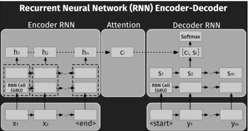
At the very high level, NMT models are comprised of an Encoder and a Decoder, both are Recurrent Neural Networks that are trained jointly. An attention mechanism helps aligning the input tokens to the output tokens in order to facilitate the translation. The Encoder reads the input sentence and generates a sequence of hidden states. These hidden

(24)

states are then used by the Decoder to generate a sequence of output words, representing the translation of the input sentence.

Figure 2.1: Neural Machine Translation model

2.1.1 RNN Encoder-Decoder

The models trained and evaluated in this thesis are based on an RNN Encoder-Decoder architecture, commonly adopted in NMT [106, 171, 59]. This model consists of two major

components: an RNN Encoder, which encodes a sequence of terms xinto a vector

repre-sentation, and an RNN Decoder, which decodes the representation into another sequence

of terms y. The model learns a conditional distribution over a (output) sequence

condi-tioned on another (input) sequence of terms: P(y1, .., ym|x1, .., xn), where n and m may

differ. In our case, we would like to learn the code transformation codebef ore→codeaf ter,

therefore given an input sequence x = codebef ore = (x1, .., xn) and a target sequence

y = codeaf ter = (y1, .., ym), the model is trained to learn the conditional distribution:

P(codeaf ter|codebef ore) =P(y1, .., ym|x1, .., xn), wherexi and yj are abstracted source

to-kens: Java keywords, separators, IDs, and idioms. Fig. 2.1 shows the architecture of the Encoder-Decoder model with attention mechanism [46, 128, 54]. The Encoder takes as

(25)

public void private boolean static void METHOD_1 boolean METHOD_1 ( ) { METHOD_1 ( ) { ( ) { if return ( time VAR_1 time ( ; ( ) ) ) > ( . equals ( == ( < ( >= ( VAR_1 VAR_1 VAR_1 ) ; ) ; ) ; } } }

publicboolean METHOD_1 () { return (time()) > (VAR_1); }

buggy code

publicboolean METHOD_1 () { return (time()) >= (VAR_1); }

fixed code

<eos>

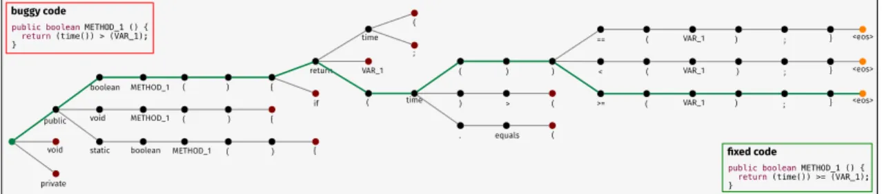
Figure 2.2: Beam Search Visualization.

on a bi-directional RNN Encoder [46], which is formed by a backward and a forward RNN, which are able to create representations taking into account both past and future inputs

[54]. That is, each state hi represents the concatenation (dashed box in Fig. 2.1) of the

states produced by the two RNNs when reading the sequence in a forward and backward

fashion: hi = [ − → hi; ←− hi].

The RNN Decoder predicts the probability of a target sequencey= (y1, .., ym)givenh.

Specifically, the probability of each output termyi is computed based on: (i) the recurrent

statesiin the Decoder; (ii) the previousi−1terms(y1, .., yi−1); and (iii) a context vectorci.

The latter constitutes the attention mechanism. The vector ci is computed as a weighted

average of the states in h: ci =Pnt=1aitht where the weightsait allow the model to pay

moreattention to different parts of the input sequence. Specifically, the weight ait defines

how much the termxi should be taken into account when predicting the target termyt.

The entire model is trained end-to-end (Encoder and Decoder jointly) by minimizing the negative log likelihood of the target terms, using stochastic gradient descent.

2.1.2 Generating Multiple Translations via Beam Search

The classic greedy decoding selects, at each time stepi, the output termyiwith the highest

probability. The downside of this decoding strategy is that, given acodebef oreas input, the

trained model will generate only one possible sequence of predictedcodeaf ter. Conversely,

we would like to generate multiple potential translations (i.e., candidates forcodeaf ter) for

a givencodebef ore. To this aim, we employ a different decoding strategy called Beam Search

(26)

Search decoding is that rather than predicting at each time step the token with the best

probability, the decoding process keeps track ofkhypotheses (withk being the beam size

or width). Formally, let H_tbe the set ofk hypotheses decoded till time stept:

Ht={(˜y11, . . . ,y˜t1),(˜y12, . . . ,y˜t2), . . . ,(˜y1k, . . . ,y˜kt)}

At the next time step t+ 1, for each hypothesis there will be |V|possible yt+1 terms

(V being the vocabulary), for a total of k· |V|possible hypotheses.

C_t₊₁ =

k

[

i=1

{(˜y₁1, . . . ,y˜_t1, v1), . . . ,(˜y1k, . . . ,y˜tk, v|V|)}

From these candidate sets, the decoding process keeps theksequences with the highest

probability. The process continues until each hypothesis reaches the special token

repre-senting the end of a sequence. We consider thesekfinal sentences as candidate patches for

the buggy code. Note that whenk= 1, Beam Search decoding coincides with the greedy

strategy.

Fig. 2.2 shows an example of the Beam Search decoding strategy with k= 3. Given

the codebef ore that represents a buggy code input (top-left), the Beam Search starts by

generating the top-3 candidates for the first term (i.e., public, void, private). At the

next time step, the beam search expands each current hyphothesis and finds that the top-3

most likely are those following the nodepublic. Therefore, the other two branches (i.e.,

void, private) are pruned (i.e., red nodes). The search continues till each hypothesis

reaches the <eos> (End Of Sequence) symbol. Note that each hypothesis could reach the

end at different time steps. This is a real example generated by our model, where one of

(27)

2.1.3 Hyperparameter Search

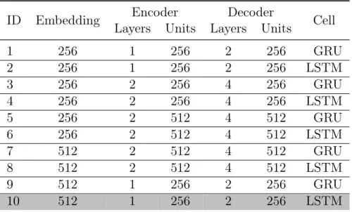
Table 2.1 shows the 10 different configurations of hyperparameters we employed when tuning the models. Each row represents a configuration with the following fields:

• ID: Configuration number;

• Embedding: the size of the embedding vector used to represent each token in the

sentence;

• Encoder and Decoder: Encoder and Decoder settings:

– Layers: number of layers;

– Units: number of units (i.e., neurons);

• Cell: Type of RNN cell used (e.g., LSTM or GRU);

Table 2.1: Hyperparameter Configurations

Encoder

Decoder

ID Embedding Layers Units Layers Units Cell

1

256

1

256

2

256

GRU

2

256

1

256

2

256

LSTM

3

256

2

256

4

256

GRU

4

256

2

256

4

256

LSTM

5

256

2

512

4

512

GRU

6

256

2

512

4

512

LSTM

7

512

2

512

4

512

GRU

8

512

2

512

4

512

LSTM

9

512

1

256

2

256

GRU

10

512

1

256

2

256

LSTM

It is worth noting that, while there can be many more possible configurations, our goal was to experiment with a diverse set of values for each parameter in a reasonable time. More fine tuning will be needed in future work. In defining the grid of hyperparameter values, we relied on the suggestions available in the literature [54], in particular, we define

(28)

the Decoder to be deeper (i.e., number of layers) than the Encoder as experimental studies

suggest.

We found that the configuration yielding the best results is the #10: 512 embedding size, 1-layer Encoder, 2-layers Decoder both with 256 neurons and LSTM cells. It is

in-teresting to note that this represents the shallowest model we tested, but with thebiggest

dimensionality of embedding size. We believe this is due to two major factors: (i) the rela-tively small number of training instances w.r.t. the model parameters makes larger models effectively not being able to generalize on new instances; (ii) a larger dimensionality will result in a more expressive representation for sentences, and in turn, better performances. In recent experiments we tested an even smaller model (based on configuration #10) with only 128 neurons for each layer with the goal of minimizing the model and obtain

better generalization. We observed a slight drop in performances (∼5%) but faster training

time. Further experiments shall be performed in order to tune the parameters of the model and find the sweet spot between size and performances.

2.1.4 Overfitting

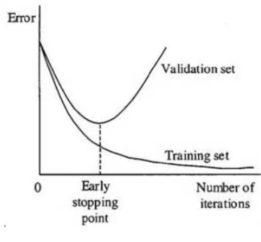
All standard neural network architectures such as the fully connected multi-layer perceptron are prone to overfitting [74]: While the network seems to get better and better, i.e., the error on the training set decreases, at some point during training it actually begins to get worse again, i.e., the error on unseen examples increases.

— Lutz Prechelt, Early Stopping - But When? [155]

This phenomenon is depicted in Figure 2.3, where the error (i.e., loss function) on the

training and validation set is observed throughout the training iterations. The error on the training set steadily decreases during the training iterations, on the other hand, the error on unseen examples belonging to the validation set starts to get worse at some point during the training. In other words, the model stops generalizing and, instead, starts learning the

(29)

statistical noise in the training dataset. This overfitting of the training dataset will result

in an increase in generalization error, making the model less useful at making predictions on new data points.

Figure 2.3: Overfitting

Intuitively, we would like to stop the training right before the model starts to overfit

on the training instances (i.e., the early stopping point in Figure 2.3).

This strategy is known as early stopping. It is probably the most commonly used form of regularization in deep learning. Its popularity is due both to its effectiveness and its simplicity.

— Goodfellowet al., Deep Learning [77]

In this work, we employ early stopping to avoid overfitting. In particular, we let the model train for a maximum of 60k iterations and select the model’s checkpoint with the

minimum error on thevalidation set – not thetraining set – and finally testing this selected

(30)

Chapter 3

Learning How to Mutate Source

Code from Bug-Fixes

3.1

Introduction

Mutation testing is a program analysis technique aimed at injecting artificial faults into

the program’s source code or bytecode [89, 64] to simulate defects. Mutants (i.e., versions

of the program with an artificial defect) can guide the design of a test suite,i.e., test cases

are written or automatically generated by tools such as Evosuite [71, 72] until a given percentage of mutants has been “killed”. Also, mutation testing can be used to assess the effectiveness of an existing test suite when the latter is already available [139, 53].

A number of studies have been dedicated to understand the interconnection between mutants and real faults [41, 42, 63, 104, 127, 166, 105, 57]. Daran and Thévenod-Fosse [63]

and Andrewset al. [41, 42] indicated that mutants, if carefully selected, can provide a good

indication of a test suite’s ability to detect real faults. However, they can underestimate

a test suite’s fault detection capability [41, 42]. Also, as pointed out by Just et al. [105],

there is a need to improve mutant taxonomies in order to make them more representative of real faults. In summary, previous work suggests that mutants can be representative of real faults if they properly reflect the types and distributions of faults that programs

(31)

exhibit. Taxonomies of mutants have been devised by taking typical bugs into account [145, 110]. Furthermore, some authors have tried to devise specific mutants for certain

domains [98, 188, 65, 146, 186]. A recent work by Brown et al. [55] leveraged bug-fixes

to extract syntactic-mutation patterns from the diffs of patches. The authors mined 7.5k types of mutation operators that can be applied to generate mutants.

However, devising specific mutant taxonomies not only requires a substantial manual effort, but also fails to sufficiently cope with the limitations of mutation testing pointed out by previous work. For example, different projects or modules may exhibit diverse distributions of bugs and types, helping to explain why defect prediction approaches do not work out-of-the-box when applied cross-project [205]. Instead of manually devising mutant taxonomies, we propose to automatically learn mutants from existing bug fixes. Such a strategy is likely to be effective for several reasons. First, a massive number of bug-fixing commits are available in public repositories. In our exploration, we found around 10M bug-fix related commits on GitHub just in the last six years. Second, a buggy code fragment arguably represents the perfect mutant for the fixed code because: (i) the buggy version is a mutation of the fixed code; (ii) such a mutation already exposed a buggy behavior; (iii) the buggy code does not represent a trivial mutant; (iv) the test suite did not detect the bug in the buggy version. Third, advanced machine learning techniques such as deep learning have been successfully applied to capture code characteristics and effectively support several SE tasks tasks [189, 196, 115, 83, 81, 158, 92, 38, 39, 35].

Stemming from such considerations, and being inspired from the work of Brown et

al. [55], we propose an approach for automatically learning mutants from actual bug

fixes. After having mined bug-fixing commits from software repositories, we extract change operations using an AST-based differencing tool and abstract them. Then, to enable learning of specific mutants, we cluster similar changes together. Finally, we learn from the changes using a Recurrent Neural Network (RNN) Encoder-Decoder architecture [106, 171, 59]. When applied to unseen code, the learned model decides in which location and what changes should be performed. Besides being able to learn mutants from an existing

(32)

source code corpus, and differently from Brown et al. [55], our approach is also able to

determine where and how to mutate source code, as well as to introduce new literals and identifiers in the mutated code.

We evaluate our approach on787kbug-fixing commits with the aim of investigating (i)

how similar the learned mutants are as compared to real bugs; (ii) how specialized models (obtained by clustering changes) can be used to generate specific sets of mutants; and (iii) from a qualitative point of view, what operators were the models able to learn. The results indicate that our approach is able to generate mutants that perfectly correspond to the original buggy code in 9% to 45% of cases (depending on the model). Most of the generated mutants are syntactically correct (more than 98%), and the specialized models are able to inject different types of mutants.

This chapter provides the following contributions:

• A novel approach for learning how to mutate source code from bug-fixes. To the best of our knowledge, this is the first attempt to automatically learn and generate mutants.

• Empirical evidence that our models are able to learn diverse mutation operators that are closely related to real bugs.

• We release the data and code to enable replication [43].

3.2

Approach

We start by mining bug-fixing commits from thousands of GitHub repositories (Sec. 3.2.1).

From the bug-fixes, we extract method-level pairs of buggy and corresponding fixed code

that we calltransformation pairs (TPs) (Sec. 3.2.2.1). TPs represent the examples we use

to learn how to mutate code from bug-fixes (fixed → buggy). We rely on GumTree [67]

to extract a list of edit actions (A) performed between the buggy and fixed code. Then,

(33)

into a representation that is more suitable for learning. The output of this phase is the

set of abstracted TPs and their corresponding mappingM which allows to reconstruct the

original source code. Next, we generate different datasets of TPs (Sec. 3.2.2.4 and 3.2.2.5). Finally, for each set of TPs we use an encoder-decoder model to learn how to transform a

fixed piece of code into the correspondingbuggy version (Sec. 3.2.3).

3.2.1 Bug-Fixes Mining

We downloaded the GitHub Archive [80] containing every public GitHub event between March 2011 and October 2017. Then, we used the Google BigQuery APIs to identify commits related to bug-fixes. We selected all the commits having a message containing the patterns: (“fix” or “solve”) and (“bug” or “issue” or “problem” or “error”). We identified 10,056,052 bug-fixing commits for which we extracted the commit ID (SHA), the project repository, and the commit message.

Since we are aware that not all commit messages matching our pattern are neces-sarily related to corrective maintenance [44, 93], we assessed the precision of the regular expression used to identify bug-fixing commits. Two authors independently analyzed a

statistically significant sample (95% confidence level ±5% confidence interval, for a total

size of 384) of identified commits to judge whether the commits were actually referring to bug-fixing activities. Next, the authors met to resolve a few disagreements in the evalua-tion (only 13 cases). The evaluaevalua-tion results, available in our appendix [43], reported a true positive rate of 97%. The commits classified as false positives mainly referred to partial and incomplete fixes.

After collecting the bug-fixing commits, for each commit we extracted the source code

pre- and post- bug-fixing (i.e., buggy and fixed code) by using the GitHub Compare API

[75]. During this process, we discarded files that were created in the bug-fixing commit, since there is no buggy version to learn from, as the mutant would be the deletion of the entire source code file. In this phase, we also discarded commits that had touched more than five Java files, since we aim to learn from bug-fixes focusing on only a few files and

(34)

not spread across the system, and as found in previous work [94], large commits are more

likely to represent tangled changes, i.e., commits dealing with different tasks. Also, we

excluded commits related to repositories written in languages different than Java, since we aim at learning mutation operators for Java code. After these filtering steps, we extracted

the pre- and post-code from ∼787k (787,178) bug-fixing commits.

3.2.2 Transformation Pairs Analysis

A TP is a pair(mb, mf)wheremb represents a buggy code component andmf represents

the corresponding fixed code. We will use these TPs as examples when training our RNN. The idea is to train the model to learn the transformation from the fixed code component

(mf) to the buggy code (mb), in order to generate mutants that are similar to real bugs.

3.2.2.1 Extraction

Given a bug-fix bf, we extracted the buggy files (fb) and the corresponding fixed (ff)

files. For each pair (fb, ff), we ran AST differencing between the ASTs of fb and ff

using GumTree Spoon AST Diff [67], to compute the sequence of AST edit actions that

transformsfb intoff.

Instead of computing the AST differencing between the entire buggy and fixed files, we separate the code into method-level pieces that will constitute our TPs. We first rely on

GumTree to establish the mapping between the nodes of fb andff. Then, we extract the

list of mapped pairs of methods L ={(m1b, m1f), . . . ,(mnb, mnf)}. Each pair (mib, mif)

contains the method mib (from the buggy filefb) and the corresponding mapped method

mif (from the fixed fileff). Next, for each pair of mapped methods, we extract a sequence

of edit actions using the GumTree algorithm. We then consider only those method pairs

for which there is at least one edit action (i.e., we disregard methods unmodified during

the fix). Therefore, the output of this phase is a list of T P s={tp1, . . . , tpk}, where each

TP is a triplettp={mb, mf, A}, wheremb is the buggy method, mf is the corresponding

(35)

consider any methods that have been newly created or completely deleted within the fixed file, since we cannot learn mutation operations from them. Also, TPs do not capture

changes performed outside methods (e.g., class name).

The rationale behind the choice of method-level TPs is manyfold. First, methods represent a reasonable target for mutation, since they are more likely to implement a single task. Second, methods provide enough meaningful context for learning mutations, such as variables, parameters, and method calls used in the method. Smaller snippets of code lack the necessary context. Third, file- or class-level granularity could be too large to learn patterns of transformation. Finally, considering arbitrarily long snippets of code, such as hunks in diffs, could make the learning more difficult given the variability in size and context [113, 33]. Note that we consider each TP as an independent fix, meaning that multiple methods modified in the same bug fixing activity are considered independently

from one other. In total, we extracted ∼2.3M TPs.

3.2.2.2 Abstraction

The major problem in dealing with raw source code in TPs is the extremely large

vocabu-lary created by the multitude of identifiers and literals used in the code of the∼2M mined

projects. This large vocabulary would hinder our goal of learning transformations of code as a neural machine translation task. Therefore, we abstract the code and generate an expressive yet vocabulary-limited representation. We use a combination of a Java lexer and parser to represent each buggy and fixed method within a TP, as a stream of tokens. First, the lexer (based on ANTLR [152, 150]) reads the raw code tokenizing it into a stream of tokens. The tokenized stream is then fed into a Java parser [185], which discerns the

role of each identifier (i.e., whether it represents a variable, method, or type name) and

the type of literals.

Each TP is abstracted in isolation. Given a TP tp = {mb, mf, A}, we first consider

the source code of mf. The source code is fed to a Java lexer, producing the stream of

(36)

literals in the stream. The parser then generates and substitutes a unique ID for each iden-tifier/literal within the tokenized stream. If an identifier or literal appears multiple times in the stream, it will be replaced with the same ID. The mapping of identifiers/literals with

their corresponding IDs is saved in a map (M). The final output of the Java parser is the

abstracted method (abstractf). Then, we consider the source code of mb. The Java lexer

produces a stream of tokens, which is then fed to the parser. The parser continues to use

mapM formb. The parser generates new IDs only for novel identifiers/literals, not already

contained in M, meaning, they exist in mb but not inmf. Then, it replaces all the

iden-tifiers/literals with the corresponding IDs, generating the abstracted method (abstractb).

The abstracted TP is now the following 4-tupletpa={abstractb, abstractf, A, M}, where

M is the ID mapping for that particular TP. The process continues considering the next

TP, generating a new mappingM. Note that we first analyze the fixed codemf and then

the corresponding buggy codemb of a TP since this is the direction of the learning process

(from mb to mf).

The assignment of IDs to identifiers and literals occurs in a sequential and positional

fashion. Thus, the first method name found will receive the ID METHOD_1, likewise the

second method name will receive ID METHOD_2. This process continues for all method

and variable names (VAR_X) and literals (STRING_X,INT_X,FLOAT_X). Figure 3.1 shows an

example of the TP’s abstracted code. It is worth noting that IDs are shared between the two versions of the methods and new IDs are generated only for newly found identifiers/literals. The abstracted code allows to substantially reduce the number of unique words in the vocabulary because we allow the reuse of IDs across different TPs. For example, the first

method name identifier in any transformation pair will be replaced with the IDMETHOD_1,

regardless of the original method name.

At this point, abstractb and abstractf of a TP are a stream of tokens consisting of

language keywords (e.g.,if), separators (e.g., “(”, “;”) and IDs representing identifiers and

(37)

public MyList checkList(MyList l){

if(l.size() < 0) populateList(l); return l;}

public MyList checkList(MyList l){

if(l.size() < 1) populateList(l); return l;}

buggy code fixed code

bug-fix mutation

public TYPE_1 METHOD_1 ( TYPE_1

VAR_1 ) { if ( VAR_1 . METHOD_2

( ) < INT_1 ) METHOD_3

( VAR_1 ) ; return VAR_1 ; }

abstracted buggy code abstracted fixed code

VAR_1 ) { if ( VAR_1 . METHOD_2

( ) < INT_2 ) METHOD_3

( VAR_1 ) ; return VAR_1 ; }

VAR_1 ) { if ( VAR_1 . size

( ) < 1 ) METHOD_2 ( VAR_1 );

return VAR_1 ; }

abstracted buggy code with idioms abstracted fixed code with idioms

VAR_1 ) { if ( VAR_1 . size

( ) < 0 ) METHOD_2 ( VAR_1 ) ;

return VAR_1 ; }

learning

Figure 3.1: Transformation Pair Example.

Figure 3.1 shows an example of a TP. The left side is the buggy code and the right side

is the same method after the bug-fix (changed theifcondition). The abstracted stream of

tokens is shown below each corresponding version of the code. Note that the fixed version is abstracted before the buggy version. The two abstracted streams share most of the

IDs, except for theINT_2ID (corresponding to the int value 0), which appears only in the

buggy version.

There are some identifiers and literals that appear so often in the source code that, for the purpose of our abstraction, they can almost be treated as keywords of the language.

For example, the variables i,j, or index are often used in loops. Similarly, literals such

as 0, 1, -1 are often used in conditional statements and return values. Method names,

such as getValue, appear multiple times in the code as they represent common concepts.

These identifiers and literals are often referred to as “idioms” [55]. We keep these idioms in our representation, that is, we do not replace idioms with a generated ID, but rather keep the original text in the code representation. To define the list of idioms, we first randomly sampled 300k TPs and considered all their original source code. Then, we extracted the frequency of each identifier/literal used in the code, discarding keywords, separators, and comments. Next, we analyzed the distribution of the frequencies and focused on the top

(38)

the distribution. Two authors manually analyzed this list and curated a set of 272 idioms.

Idioms also include standard Java types such as String, Integer, common Exceptions,

etc. The complete list of idioms is available on our online appendix [43].

Figure 3.1 shows theidiomized abstracted code at the bottom. The method namesize

is now kept in the representation and not substituted with an ID. This is also the case for

the literal values 0 and 1, which are very frequent idioms. Note that the method name

populateList is now assigned ID METHOD_2 rather than METHOD_3. This representation

provides enough context and information to effectively learn code transformations, while

keeping a limited vocabulary (|V|=∼430). Note that the abstracted code can be mapped

back to the real source code using the the mapping (M).

3.2.2.3 Filtering Invalid TPs

Given the extracted list of 2.3M TPs, we manipulated their code via the aforementioned abstraction method. During the abstraction, we filter out such TPs that: (i) contain

lexical or syntactic errors (i.e., either the lexer or parser failed to process them) in either

the buggy or fixed version of the code; (ii) their buggy and fixed abstracted code (abstractb,

abstractf) resulted in equal strings. The equality of abstractb and abstractf is evaluated

while ignoring whitespace, comments or annotations edits, which are not useful in learning mutants. Next, we filter out TPs that performed more than 100 atomic AST actions

(|A|>100) between the buggy and fixed version. The rationale behind this decision was

to eliminate outliers of the distribution (the 3rd quartile of the distribution is 14 actions) which could hinder the learning process. Moreover, we do not aim to learn such large mutations. Finally, we discard long methods and focus on small/medium size TPs. We filter out TPs whose fixed or buggy abstracted code is longer than 50 tokens. We discuss this choice in the Section 3.5 and report preliminary results also for longer methods. After

(39)

3.2.2.4 Synthesis of Identifiers and Literals

TPs are the examples we use to make our model learn how to mutate source code. Given a

tp={mb, mf, A}, we first abstract its code, obtainingtpa={abstractb, abstractf, A, M}.

The fixed code abstractf is used as input to the model which is trained to output the

corresponding buggy code (mutant) abstractb. This output can be mapped back to real

source code using M.

In the current usage scenario (i.e., generating mutants), when the model is deployed,

we do not have access to the oracle (i.e., buggy code, abstractb), but only to the input

code. This source code can then be abstracted and fed to the model, which generates as

output a predicted code (abstractp). The IDs that theabstractp contains can be mapped

back to real values only if they also appear in the input code. If the mutated code suggests

to introduce a method call, METHOD_6, which is not found in the input code, we cannot

automatically map METHOD_6 to an actual method name. This inability to map back

source code exists for any newly created ID generated for identifiers or literals, which are absent in the input code. Synthesizing new identifiers would involve extensive knowledge about the project, control and data flow information. For this reason, we discard the TPs

that contain, in the buggy method mb, new identifiers not seen in the fixed method mf.

The rationale is that we want to train our model from examples that rearrange existing identifiers, keywords and operators to mutate source code. Instead, this is not the case for literals. While we cannot perfectly map a new literal ID to a concrete value, we can still synthesize new literals by leveraging the type information embedded in the ID. For

example, the (fixed) if condition in Figure 3.1 if(VAR_1.METHOD_2( ) < INT_1) should

be mutated in its buggy version if(VAR_1.METHOD_2( ) < INT_2). The value of INT_2

has never appeared in the input code (fixed), but we could still generate a compilable mutant by randomly generating a new integer value (different from any literal in the input code). While in these cases the literal value is randomly generated, the mutation model still provides the prediction about which literal to mutate.

(40)

For such reasons, we create two sets of TPs, hereby referred asT Pident andT Pident−lit.

T Pident contains all TPs tpa= {abstractb, abstractf, A, M} such that every identifier ID

(VAR_, METHOD_, TYPE_) in abstractb is found also in abstractf. In this set we do allow

new literal IDs (STRING_, INT_, etc.). T Pident−lit is a subset of T Pident, which is more

restrictive, and only contains the transformation pairstpa={abstractb, abstractf, A, M}

such that every identifier and literal ID inabstractb is found also inabstractf. Therefore,

we do not allow new identifiers nor literals.

The rationale behind this choice is that we want to learn from examples (TPs) where

the model is able to generate compilable mutants (i.e., generate actual source code, with

real values for IDs). In the case of the T Pident−lit set, the model will learn from examples

that do not introduce any new identifier and literal. This means that the model will likely generate code for which every literal and identifier can be mapped to actual values. From

the set T Pident the model will likely generate code for which we can map every identifier

but we may need to generate new random literals.

In this context it is important to understand the role played by the idioms in our code representation. Idioms help to retain transformation pairs that we would otherwise discard, and learn transformation of literal values that we would otherwise need to randomly

gen-erate. Consider again the previous example if(VAR_1 . METHOD_2 ( ) < INT_1) and

its mutated versionif(VAR_1 . METHOD_2 ( ) < INT_2). In this example, there are no

idioms and, therefore, the model learns to mutateINT_1to INT_2within theifcondition.

However, when we want to map back the mutated (buggy) representation to actual source

code, we will not have a value for INT_2 (which does not appear in the input code) and,

thus, we will be forced to generate a synthetic value for it. Instead, with the idiomized

abstract representation the model would treat the idioms0 and 1 as keywords of the

lan-guage and learn the exact transformation of the ifcondition. The proposed mutant will

therefore contain directly the idiom value (1) rather thanINT_2. Thus, the model will learn

and propose such transformation without the need to randomly generate literal values. In summary, idioms increase the number of transformations incorporating real values rather

(41)

than abstract representations. Without idioms, we would lose these transformations and our model could be less expressive.

3.2.2.5 Clustering

The goal of clustering is to create subsets of TPs such that TPs in each cluster share a similar list of AST actions. Each cluster represents a cohesive set of examples so that a trained a model can apply those actions to a new code.

As previously explained, each transformation pair tp = {mb, mf, A} includes a list

of AST actions A. In our dataset, we found ∼1,200 unique AST actions, and each TP

can perform a different number and combination of these actions. Deciding whether the

transformation pairs,tp1 and tp2, perform a similar sequence of actions and, thus, should

be clustered together, is far from trivial. Possible similarity functions include the number of shared elements in the two sets of actions and the frequency of particular actions within the sets. Rather than defining such handcrafted rules, we choose to learn similarities directly from the data. We rely on an unsupervised learning algorithm that learns vector

representations for the lists of actions A of each TP. We treat each list of AST actions

(A) as a document and rely on doc2vec [161] to learn a fixed-size vector representation

of such variable-length documents embedded in a latent space where similarities can be computed as distances. The closer two vectors are, the more similar the content of the two corresponding documents. In other words, we mapped the problem of clustering TPs

to the problem of clustering continuous valued vectors. To this goal, we use k-means

clustering, requiring the number of clusters (k) into which to partition the data upfront.

When choosing k, we need to balance two conflicting factors: (i) maximize the number

of clusters so that we can train several different mutation models and, as a consequence, apply different mutations to a given piece of code; and (ii) have enough training examples (TPs) in each cluster to make the learning possible. Regarding the first point, we target at least three mutation models. Concerning the second point, with the available TPs dataset we could reasonably train no more than six clusters, so that each of those contain enough

(42)

TPs. Thus, we experiment on the dataset T Pident−lit with values of k going from 3 to 6

at steps of 1 and we evaluate each clustering solution in terms of its Silhouette statistic

[107, 112], a metric used to judge the quality of clustering. We found thatk= 5generates

the clusters with the best overall Silhouette values. We cluster the datasetT Pident−lit into

clusters: C1, C2, C3, C4, C5.

3.2.3 Learning Mutations

3.2.3.1 Dataset Preparation

Given a set of TPs (i.e., T Pident, T Pident−lit, C1, . . . , C5) we use the instances to train

our Encoder-Decoder model. Given a tpa={abstractb, abstractf, A, M} we use only the

pair (abstractf, abstractb) of fixed and buggy abstracted code for learning. No additional

information about the possible mutation actions (A) is provided during the learning process

to the model. The given set of TPs is randomly partitioned into: training (80%), evaluation (10%), and test (10%) sets. Before the partitioning, we make sure to remove any duplicated

pairs (abstractf, abstractb) to not bias the results (i.e., same pair both in training and test

set).

3.2.3.2 Encoder-Decoder Model

Our models are based on an RNN Encoder-Decoder architecture, commonly adopted in Machine Translation [106, 171, 59]. This model comprises two major components: an

RNN Encoder, which encodes a sequence of terms x into a vector representation, and

an RNN Decoder, which decodes the representation into another sequence of terms y.

The model learns a conditional distribution over a (output) sequence conditioned on

an-other (input) sequence of terms: P(y1, .., ym|x1, .., xn), where n and m may differ. In

our case, given an input sequence x = abstractf = (x1, .., xn) and a target sequence

y = abstractb = (y1, .., ym), the model is trained to learn the conditional distribution:

(43)

tokens: Java keywords, separators, IDs, and idioms. The Encoder takes as input a

se-quence x = (x1, .., xn) and produces a sequence of states h = (h1, .., hn). We rely on

a bi-directional RNN Encoder [46] which is formed by a backward and forward RNNs, which are able to create representations taking into account both past and future inputs

[54]. That is, each statehi represents the concatenation of the states produced by the two

RNNs reading the sequence in a forward and backward fashion: hi = [

− →

hi;

←−

hi]. The RNN

Decoder predicts the probability of a target sequencey= (y1, .., ym)givenh. Specifically,

the probability of each output termyi is computed based on: (i) the recurrent statesi in

the Decoder; (ii) the previous i−1 terms (y1, .., yi−1); and (iii) a context vector ci. The

latter practically constitutes the attention mechanism. The vector ci is computed as a

weighted average of the states inh, as follows: ci =Pnt=1aithtwhere the weightsait allow

the model to pay moreattention to different parts of the input sequence. Specifically, the

weight ait defines how much the term xi should be taken into account when predicting

the target termyt. The entire model is trained end-to-end (Encoder and Decoder jointly)

by minimizing the negative log likelihood of the target terms, using stochastic gradient descent.

3.2.3.3 Configuration and Tuning

For the RNN Cells we tested both LSTM [96] and GRU [59], founding the latter to be slightly more accurate and faster to train. Before settling on the bi-directional Encoder, we tested the unidirectional Encoder (with and without reversing the input sequence), but we consistently found the bi-directional one yielding more accurate results. Bucketing and padding was used to deal with the variable length of the sequences. We tested several combinations of the number of layers (1,2,3,4) and units (256, 512). The configuration that best balanced performance and training time was the one with 1 layer encoder, 2 layer decoder both with 256 units. We train our models for 40k epochs, which represented our empirically-based sweet spot between training time and loss function improvements. The evaluation step was performed every 1k epochs.

(44)

3.3

Experimental Design

The evaluation has been performed on the dataset of bug fixes described in Section??and

answers three RQs.

RQ1: Can we learn how to generate mutants from bug-fixes? RQ1 investigates

the extent to which bug fixes can be used to learn and generate mutants. We train models

based on the two datasets: T Pident and T Pident−lit. We refer to such models with the

name general models (GMident,GMident−lit), because they are trained using TPs of each

dataset without clustering. Each dataset is partitioned into 80% training, 10% validation, 10% testing.

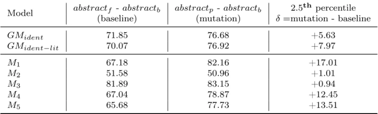
BLEU Score. The first performance metric we use is the Bilingual Evaluation

Under-study (BLEU) score, a metric used to assess the quality of a machine translated sentence [149]. BLEU scores require reference text to generate a score, which indicates how similar the candidate and reference texts are. The candidate and reference texts are broken into n-grams and the algorithm determines how many n-grams of the candidate text appear in the reference text. We report the global BLEU score, which is the geometric mean of all n-grams up to four. To assess our mutant generation approach, we first compute the

BLEU score between the abstracted fixed code (abstractf) and the corresponding target

buggy code. This BLEU score serves as our baseline for comparison. We compute the

BLEU score between the predicted mutant (abstractp) and the target (abstractb). The

higher the BLEU score, the more similar abstractp is to abstractb,i.e., the actual buggy

code. To fully understand how similar our prediction is to the real buggy code, we need to

compare the BLEU score with our baseline. Indeed, the input code (i.e., the fixed code)

provided to our model can be considered by itself as a “close translation” of the buggy code, therefore, helping in achieving a high BLEU score. To avoid this bias, we compare the BLEU score between the fixed code and the buggy code (baseline) with the BLUE

score obtained when comparing the predicted buggy code (abstractp) to the actual buggy

(45)

one between abstractf and abstractb, it means that the model transforms the input code

(abstractf) into a mutant (abstractp) that is closer to the buggy code (abstractb) than it

was before the mutation, i.e., the mutation goes in the right direction. In the opposite

case, the predicted code represents a translation that is further from the buggy code when compared to the original input. To assess whether the differences in BLEU scores between the baseline and the models are statistically significant, we employ a technique devised

by Zhang et al. [203]. Given the test set, we generate m = 2,000 test sets by sampling

with replacement from the original test set. Then, we evaluate the BLEU score on the

m test sets both for our model and the baseline. Next, we compute the m deltas of the

scores: δi =modeli−baselinei. Given the distribution of the deltas, we select the 95%

confidence interval (CI) (i.e., from the 2.5th percentile to the 97.5th percentile). If the CI

is completely above or below the zero (e.g.,2.5th percentile> 0) then the differences are

statistically significant.

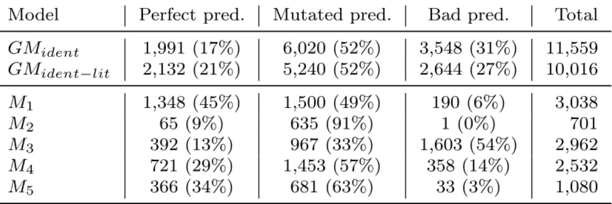
Prediction Classification. Given abstractf, abstractb and abstractp, we classify each

prediction into one of the following categories: (i) perfect prediction ifabstractp=abstractb

(the model converts the fixed code back to its buggy version, thus reintroducing the

original bug); (ii) bad prediction if abstractp = abstractf (the model was not able to

mutate the code and returned the same input code); and (iii) mutated prediction if

abstractp 6= abstractb AND abstractp 6= abstractf (the model mutated the code, but

differently than the target buggy code). We report raw numbers and percentages of the predictions falling in the described categories.

Syntactic Correctness. To be effective, mutants need to be syntactically correct,

allow-ing the project to be compiled and tested against the test suite. We evaluate whether the models’ predictions are lexically and syntactically correct by means of a Java lexer and parser. Perfect predictions and bad predictions are already known to be syntactically cor-rect, since we established the correctness of the buggy and fixed code when extracting the TPs. The correctness of the predictions within the mutated prediction category is instead unknown. For this reason, we report both the overall percentage of syntactically correct

(46)

predictions as well as the mutated predictions. We do not assess the compilability of the code.

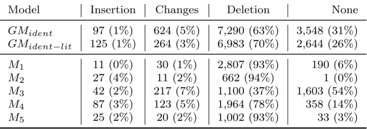
Token-based Operations. We analyzed and classified models’ predictions also based on

their tokens’ operations, classifying the predictions into one of four categories: (i) insertion

if #tokens predictions>#tokens input; (ii) changes if #tokens prediction = #tokens input

AND prediction6= input; (iii) deletions if #tokens prediction<#tokens input; (iv) none

if prediction = input. This analysis aims to understand whether the models are able to insert, change or delete tokens.

AST-based Operations. Next, we focus on the mutated predictions. These are not

perfect predictions, but we are interested in understanding whether the transformations performed by the models are somewhat similar to the transformations between the fixed and buggy code. In other words, we investigate whether the model performs AST ac-tions similar to the ones needed to transform the input (fixed) code into the corresponding

buggy code. Given the input fixed codeabstractf, the corresponding buggy codeabstractb,

and the predicted mutant abstractp, we extract with GumTreeDiff the following lists of

AST actions: Af−b = actions(abstractf → abstractb) and Af−p = actions(abstractf →

abstractp). We then compare the two lists of actions, Af−b and Af−p, to assess their

similarities. We report the percentage of mutated predictions whose list of actions Af−p

contains the same elements and frequency of those found inAf−b. We also report the

per-centage of mutated predictions when only comparing their unique actions and disregarding their frequency. In those cases, the model performed the same list of actions but possibly in a different order, location or frequency than those which led to the perfect prediction (buggy code).

RQ2: Can we train different mutation models? RQ2 evaluates the five models

trained using the five clusters of TPs. For each model, we evaluate its performance on the corresponding 10% test set using the same analyses discussed for RQ1. In addition, we evaluate whether models belonging to different clusters generate different mutants. To this aim, we first concatenate the test set of each cluster into a single test set. Then, we

(47)

feed each input instance in the test set (fixed code) to each and every mutation model

M1, .., M5, obtaining five mutant outputs. After that, we compute the number of unique

mutants generated by the models. For each input, the number of unique mutants ranges from one to five depending on how many models generate the same mutation. We report the distribution of unique mutants generated by the models.

RQ3: What are the characteristics of the mutants generated by the

mod-els? RQ3 qualitatively assesses the generated mutants through manual analysis. We first

discuss some of the perfect predictions found by the models. Then, we focus our attention on the mutated pred