Original citation:
Andrinopoulos, Lampros, Hine, Nicholas and Mostofi, Arash A.. (2011) Calculating dispersion interactions using maximally localized Wannier functions. Journal of Chemical Physics, 135 (15). 154105 .
Permanent WRAP URL:
http://wrap.warwick.ac.uk/78160
Copyright and reuse:
The Warwick Research Archive Portal (WRAP) makes this work by researchers of the University of Warwick available open access under the following conditions. Copyright © and all moral rights to the version of the paper presented here belong to the individual author(s) and/or other copyright owners. To the extent reasonable and practicable the material made available in WRAP has been checked for eligibility before being made available.
Copies of full items can be used for personal research or study, educational, or not-for profit purposes without prior permission or charge. Provided that the authors, title and full bibliographic details are credited, a hyperlink and/or URL is given for the original metadata page and the content is not changed in any way.
Publisher’s statement:
This article may be downloaded for personal use only. Any other use requires prior permission of the author and AIP Publishing.
The following article appeared in Journal of Chemical Physics and may be found at
http://dx.doi.org/10.1063/1.3647912
A note on versions:
The version presented here may differ from the published version or, version of record, if you wish to cite this item you are advised to consult the publisher’s version.
Calculating Dispersion Interactions using Maximally
Localised Wannier Functions
Lampros Andrinopoulos,1 Nicholas D. M. Hine,1 and Arash A. Mostofi1
The Thomas Young Centre for Theory and Simulation of Materials,
Imperial College London, London SW7 2AZ, UK
(Dated: May 25, 2011)
We investigate a recently developed approach1,2 that uses maximally-localized Wan-nier functions (MLWFs) to evaluate the van der Waals (vdW) contribution to the total energy of a system calculated with density-functional theory (DFT). We test it on a set of atomic and molecular dimers of increasing complexity (argon, methane, ethene, benzene, phthalocyanine, and copper phthalocyanine) and demonstrate that the method, as originally proposed, has a number of shortcomings that hamper its predictive power. In order to overcome these problems, we have developed and im-plemented a number of significant improvements to the method and show that these modifications give rise to calculated binding energies and equilibrium geometries that are in markedly closer agreement to results of quantum-chemical coupled-cluster cal-culations.
31.15.E-,71.15.Mb,34.20.Gj,31.15.-p,31.15.A-I. INTRODUCTION
Local and semi-local exchange-correlation functionals used in density-functional theory3,4 (DFT) can not account for the effect of long-ranged dispersion, or van der Waals (vdW), in-teractions. Dispersion interactions are crucial for weakly-bound systems, particularly where no covalent or ionic bonding is present, and often dominate intermolecular binding energies and equilibrium geometries. Incorporating vdW interactions in DFT remains a challenging task and a wide variety of methods have been developed, approaching the problem from many different perspectives5–13. In this work we focus on the method recently proposed by Silvestrelli1,2, which has been recently applied to various systems14–17 and implemented in a number of modern electronic structure codes18,19. This approach uses maximally-localized Wannier functions20 (MLWFs) as a means of decomposing the electronic density of the sys-tem into a set of localized but overlapping fragments, which may then be used to calculate a vdW correction to the DFT total energy by considering pairwise interactions between density fragments as derived by Andersson, Langreth and Lundqvist7 (ALL).
In this Article, we explore the parameters and approximations involved in Silvestrelli’s method and improve its results where possible by modifying various aspects of the method. We apply the method and our proposed modifications to a series of test systems, then to two more challenging systems, a phthalocyanine and a copper phthalocyanine dimer. We thus demonstrate that although this method can offer an easily implementable and computationally efficient way of calculating the dispersion correction to the energy with the possibility of improved accuracy (once some modifications are applied to it), it is largely dependent on a number of parameters and choices one can make.
II. THEORETICAL BACKGROUND
A. Maximally-Localized Wannier Functions
Wannier functions21 are orthogonal localized functions that span the same space as the eigenstates of a single particle Hamiltonian. Consider the set of Nocc occupied (valence) eigenstates {|umi} of a molecule. The total energy is invariant with respect to unitary
transformations among the eigenstates
|wni= X
m
Umn|umi. (1)
If the unitary matrix U is chosen such that the resulting Nocc orbitals {wn(r)} minimize their total quadratic spread, given by
Ω =X
n
hwn|r2|wni − hwn|r|wni2
=X
n
hr2
in−¯r2n
, (2)
then they are said to be maximally-localized Wannier functions20 (MLWFs). Each MLWF is characterized by a value for its quadratic spread, S2
n, and its centre, ¯rn.
In the construction of MLWFs it is sometimes useful to consider not only the valence manifold but also a range of unoccupied eigenstates above the Fermi level — often those constituting the antibonding counterparts to the valence states. This not only allows the MLWFs to be more localized22,23 but can also restore symmetries that would otherwise be broken arbitrarily through the construction of MLWFs for the valence manifold only.
In order to do so, one defines an outer energy window consisting of Nwin > Nocc states, from which one may extract an optimal N-dimensional subspace (Nwin > N > Nocc) using the disentanglement approach described in Ref. 24,
|uopt
m i=
Nwin
X
p=1
Udis
pm|upi, (3)
where Udis is a rectangular Nwin×N unitary matrix. N MLWFs may then be localized by suitable rotation of the optimal subspace in the usual manner:
|wni= N X
m=1
Umn|uoptm i. (4)
Furthermore, an inner, orfrozen, energy window may be defined if one wishes to make certain
inner window is set to encompass the occupied states. Algorithms for determining MLWFs from the eigenstates obtained from electronic structure calculations are implemented within the Wannier90 software package25.
When states above the Fermi level are included, there are necessarily more MLWFs than there are occupied states, so some of them will have less than full occupancy. To use these MLWFs in a decomposition of the density,
ρ(r) = N X
n=1
fnw|wn(r)|2, (5)
we need the occupancyfw
n of each. fnw is given by the expectation value of the single-particle
density operator ρˆ, which is a projection operator for the occupied manifold, with respect to|wni,
fnw =hwn|ρˆ|wni= Nocc
X
m=1
hwn|umihum|wni. (6)
Using Eq. (3) and (4), and the mutual orthonormality of the eigenstates, it may be shown that
fnw =
Nocc X i=1 N X l,m=1
Umn∗ U∗dis
im UlnUildis. (7)
We have adapted the Wannier90 code to calculate these occupancies so that they can be used where they are required in our adapted form of Silvestrelli’s method, which we describe in Sec. III.
B. Silvestrelli’s method
Silvestrelli’s approach1,2 is based on the Andersson, Langreth and Lundqvist7 (ALL) expression for the vdW energy in terms of pairwise interactions between density fragments
ρn(r)and ρl(r′), separated by a distance rnl,
EvdW=−
X
n>l
fnl(rnl)
C6nl
r6
nl
(8)
where fnl(rnl)is a damping function2 which screens the unphysical divergence of Eq. (8) at
short range, and
C6nl =
3 4(4π)3/2
ˆ
V
dr ˆ
V′
dr′
p
ρn(r)ρl(r′) p
ρn(r) + p
ρl(r′)
in atomic units. It should be noted that these expressions are only strictly valid in the limit of non-overlapping density fragments. There are various forms for the damping function26,27 that might have a slight short-range effect but should not affect the long-range behaviour of the vdW energies. Here we chose to use the damping function as proposed in the original paper by Silvestrelli1.
Now, the MLWFs obtained from the valence orbitals of a system provide a localized decomposition of the electronic charge density, such that ρn(r) = |wn(r)|2, so that Eq.( 9)
becomes:
C6nl =
3 32π3/2
ˆ
|r|≤rc
dr ˆ
|r′|≤rc′
dr′ |wn(r)||wl(r ′)|
|wn(r)|+|wl(r′)|
, (10)
whererc is a suitably chosen cutoff radius obtained by equating the length scale for density
change to the electron gas screening length2; we will revisit this point later.
In order to make the calculation of the integrals more tractable, the charge density is approximated by replacing each MLWFwn(r)with a hydrogenics-orbital that has the same
centre ¯rn and spread Sn as the MLWF, and whose analytic form is well-known and is given by
wn(r) =
33/4 √
πSn3/2
e−√3|r−¯rn|/Sn
, (11)
which, on substitution into Eq. (10) and after some algebra, gives
C6nl =
Sn3/2Sl3
2·35/4F(Sn, Sl), (12) where
F(Sn, Sl) =
ˆ xc
0
dx
ˆ yc
0
dy x
2y2e−xe−y
e−x/β+e−y, (13)
β = (Sn/Sl)3/2, xc =
√
3rc/Sn and yc =
√ 3r′
c/Sl. Eq. (13) may be evaluated easily since it
depends solely on the MLWF spreads and centres, not their detailed shapes or orientations. We note that in the case of spin degeneracy, since every MLWF is doubly occupied, the density of each fragment is multiplied by a factor of 2 and, therefore, the C6nl integral in
Eq. (10) is scaled by a factor of √2.
III. IMPROVEMENTS TO SILVESTRELLI’S METHOD
A. Partly Occupied Wannier Functions
Using a manifold of eigenstates that includes but is larger than the subspace spanned by just the valence states results in partly-occupied MLWFs that are generally more local-ized and that better reflect the symmetries of the system, as opposed to MLWFs obtained by rotation of the valence subspace only, which arbitrarily break the symmetry (we will demonstrate examples of this phenomenon in Sec. IV).
In order to account for the partial occupancy of the MLWFs, we make a slight modifi-cation to Silvestrelli’s approach, explicitly introducing occupancies in the definition of the
C6nl integral; since the density of each fragment is now given by ρn(r) = fnw|wn(r)|2, the
expression forF(Sn, Sl)in Eq. (13) becomes
F(Sn, Sl) =
ˆ xc
0
dx
ˆ yc
0
dy x
2y2e−xe−y
e−x/(βp
fw
n) +e−y/ p
fw l
, (14)
where the fw
n are given by Eq. (7). We will see in Sec. IV that this seemingly simple idea
can give rise to a marked improvement in the accuracy of the method.
B. Modification to describe p-like states
MLWFs describing only the valence manifold often take the form of well-localized func-tions centred on a bond between two atoms, and are thus reasonably well-described by the approximation of replacing them with a suitable s-orbital. When anti-bonding states are
included in the construction of the MLWFs, the resulting orbitals have more atomic-orbital character. This is demonstrated by the atom-centred p-like MLWF shown in Fig. 1 for an
ethene molecule. It is clear that the density associated with such an MLWF will not be very well represented by a single s-like function at its centre. In order to approximate p
-like orbitals appropriately when calculatingC6, one could imagine using a suitably-oriented
analytic expression for a hydrogenic p-orbital, for example, a canonical pz-orbital, given by
pz(r) =
305/4rcosθ √
32πS5/2 e
−√30r/2S, (15)
which has been normalized such that its quadratic spread ishpz|(r−¯r)2|pzi=S2. As a
evaluation of these integrals, for realistic systems, would be prohibitively computationally expensive. We solve this problem by identifying thep-like MLWFs in the system and
replac-ing them with the hydrogenic form given in Eq. (15). Then, we further approximate each lobe (lower and upper) of this p-like orbital with two separate hydrogenic s-orbitals of the
form of Eq. (11). In order to do so, it is necessary to know the spreads S± and centres ¯r± of the two lobes of the orbital separately, given by
S2 ± =
ˆ ∞
0
ˆ π/2
0
ˆ 2π
0
r4p2
z(r) sinθdrdθdφ, (16)
¯r± = ¯r ± ˆ ∞
0
ˆ π/2
0
ˆ 2π
0
r3cosθ p2
z(r) sinθdrdθdφˆz, (17)
which, after some algebra, gives
S±= 7S
8√2, (18)
¯
r±= ¯r± 15S
8√30 ˆz, (19)
where¯randSare the original centre and spread, respectively, of the MLWF. For an arbitrary orientation of the lobes of a pz-like state, we need only rotate the offset vectors (¯r±−¯r) accordingly.
Thus, we have developed a formalism whereby the charge density due to MLWFs with
p-like character can be represented by a pair of s-like hydrogenic orbitals with appropriate
centres and spreads. In Sec. IV we will show how this works in practice for calculating vdW energy corrections.
In the relatively simple systems studied in this paper, thep-like orbitals are easily
distin-guished from other orbitals by their partial occupancies, given by Eq. 7, which are typically closer to 0.5 rather than 1. Alternatively, and especially for structurally more complex sys-tems, the shape of each MLWF could be characterized using the efficient method described in Appendix A of Ref. 28 as another means of automating the procedure ofidentifyingp-like
states.
C. Symmetry Considerations
Figure 1. Partly occupiedp-like orbital on ethene molecule. In the method described here, each of
the two lobes (coloured red and blue) is replaced by ansorbital and considered a separate fragment.
optimization from a chosen initial guess. This is often enough to uniquely determine the MLWFs. In some cases, however, it does not give rise to a unique choice, even if the op-timization procedure is perfect. For example, the atomic positions and electron density of the system may possess certain symmetry elements, such as rotations about a particular axis. Then there will exist a number of equally valid and degenerate representations of the MLWFs and their centres, which give the same spread, and are related by symmetry. The minimization procedure breaks the symmetry by choosing one of these representations; in other words there will be a degree of arbitrariness in the final MLWFs. It is clear from Eq. (8) that any degree of non-uniqueness of the centres will cause an undesirable variability of the vdW energy calculated in Silvestrelli’s method. This is indeed what we observe in some of the examples below. Moving away from a description of the MLWFs using the valence states only, and towards using partly occupied MLWFs that include anti-bonding states and which retain the symmetries of the system, enables us to overcome these problems, as we demonstrate below.
IV. APPLICATIONS
A. Calculation Details
to both the semi-empirical DFT+D method29,30 as implemented in QE, which is expected to give good asymptotic behaviour, and a wavefunction-based coupled-cluster approach, CCSD(T), which is considered the ‘gold-standard’ of quantum chemistry.
The PBE31 generalized-gradient approximation for exchange and correlation, except in the case of argon where the revPBE32 functional was used; norm-conserving pseudopoten-tials, and Γ-point sampling of the Brillouin zone were used throughout. A plane-wave basis set cut-off energy of 80 Ry was used in all calculations with QE except for the case of the phthalocyanine and copper phthalocyanine where a 50 Ry energy cutoff was used. For the dimers of argon, methane, ethene, phthalocyanine and copper phthalocyanine, cubic simu-lation cells of length 15.87 Å, 15.87 Å, 21.16 Å and 23.81 Å, respectively, were used. For the dimers of benzene, a hexagonal cell with a= 15.87Å and c= 31.75 Å was used.
B. Argon
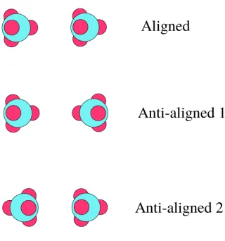
We will first investigate the severity of the aforementioned issues relating to symmetry, by considering the case of an argon dimer. Optimization of the MLWFs describing a single argon atom produces four doubly occupied MLWFs arranged tetrahedrally around the atom. Due to spherical symmetry, the orientation of these MLWFs with respect to a given coordinate system is arbitrary for an isolated atom and the final MLWFs obtained will depend on the initial guess used. In the dimer, this arbitrariness is removed, at least in principle, since the spherical symmetry is broken by the presence of the other atom at a specific orientation. At large separations, this is not in practice necessarily the case: the electron density overlap between the Ar atoms is vanishingly small, since the wavefunctions decay exponentially away from the atom. Therefore, to within attainable numerical precision, the orientation of the MLWFs on each atom is uncorrelated with the orientation of the other atom: the MLWFs can be freely rotated with respect to the atom without affecting the total spread. Note, however, that since the vdW energy only decays as R−6, its value is influenced by the orientation of the MLWF centres (and hence their separation) out to distances beyond which the calculated spread (and thus the optimised MLWF orientation) has ceased to be sensitive to separation.
Figure 2. Illustration of three of the many possible configurations of MLWF centres (small pink
spheres) for the two argon atoms (large blue spheres) in the fragment method.
calculating the MLWF centres for a single atom of argon and then translating and rotating these centres to the second Ar atom with various choices of alignment. We will refer to this approach as the fragment method. In this method, we calculate the dispersion correction to
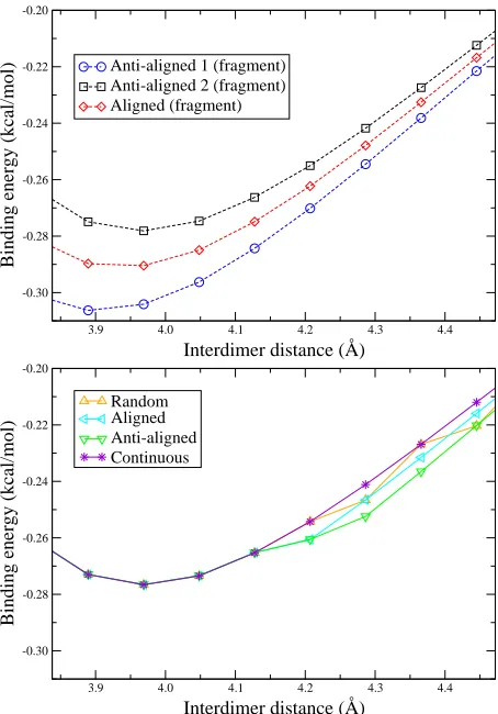
the energy for a dimer system using various possible arrangements of MLWF centres on the other atom. Three possible high-symmetry choices are shown in Fig. 2. For each of these orientations, Fig. 3 (top) shows the binding energy of the Ar dimer as the separation of the atoms varies. We see that there is considerable displacement of the curves, and the binding energy and the equilibrium separation change according to the alignment chosen by up to
0.04kcal/mol and 0.08 Å respectively.
In contrast to this fragment approach, in Fig. 3 (bottom) we show the binding energy as calculated with the normal approach of using the optimized MLWFs of the entire dimer system. However, here we have used varying initial guesses corresponding to the set of possible alignments shown in Fig. 2. We see that at small separations, the MLWF centres always converge to the same positions, regardless of the initial guess, and the binding energy curve is nearly independent of the choice of initial guess (∼10−3 kcal/mol variation).
the fragment method. This is because the MLWF centres converge to different orientations depending on their starting positions (curve labelled ‘random’ in Fig. 3 (bottom)).
In order to avoid this problem of non-uniqueness of binding energy curves, a random initial guess is used first for a configuration at small separation, in the knowledge that the result will be independent of the guess used. Then the centres computed at the previous, smaller separation are used as the initial guess for the calculation at a larger separation. In this manner, a unique continuous curve is obtained (labelled ‘continuous’ in Fig. 3 (bottom)). This is the approach that we adopt for all subsequent calculations in this paper.
From the continuous curve, we obtain 3.97 Å for the equilibrium separation and−0.28kcal/mol for the binding energy. This is in good agreement with the coupled cluster CCSD(T) cal-culations of Ref. 33, which give 3.78 Å and −0.28 kcal/mol, respectively, whereas revPBE without dispersion corrections gives 4.62 Å and −0.04 kcal/mol.
C. Methane
The methane dimer is a straightforward application of the Silvestrelli method: the po-sitions of the MLWF centres, which lie on the four tetrahedral C-H bonds of each CH4 molecule (see Fig. 4), obey the same symmetries as the atomic positions, so there exists no arbitrariness of orientation.
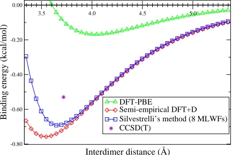
In Fig. 5, we compare to the results of both DFT+D and CCSD(T) calculations. Our geometries and CCSD(T) results were drawn from the Benchmark Energy and Geometry Database (BEGDB)34.
The accuracy of Silvestrelli’s method in the case of the methane dimer is good compared to CCSD(T): the former gives an equilibrium separation of 3.66 Å and binding energy of −0.69 kcal/mol, and the latter 3.72 Å and −0.53 kcal/mol, respectively. DFT+D is in somewhat worse agreement with CCSD(T), yielding 3.54 Å and−0.76kcal/mol, respectively.
D. Ethene
3.9 4.0 4.1 4.2 4.3 4.4 Interdimer distance (Å)
-0.30 -0.28 -0.26 -0.24 -0.22 -0.20
Binding energy (kcal/mol)
Anti-aligned 1 (fragment) Anti-aligned 2 (fragment) Aligned (fragment)
3.9 4.0 4.1 4.2 4.3 4.4
Interdimer distance (Å) -0.30
-0.28 -0.26 -0.24 -0.22 -0.20
Binding energy (kcal/mol)
[image:13.595.192.419.70.395.2]Random Aligned Anti-aligned Continuous
Figure 3. Binding energy versus interatomic separation for the argon dimer, for varying relative
orientations of the MLWF centres surrounding each atom (see Fig. 2). Top panel: results obtained
using the fragment method, in which the MLWF centres are calculated for a lone Ar atom and
then translated and rotated to the second Ar atom. Bottom panel: results obtained using the true
MLWF centres with various initial guesses for their positions. The curve labelled ‘continuous’ is
obtained by using the MLWF centres from a configuration at small separation as the initial guess
for the centres at larger separations. In this way, the discontinuities in the curve are avoided and
a unique curve is obtained (see text for details).
(BEGDB)34.
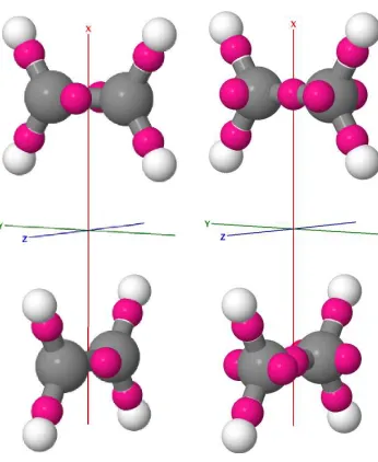
To use Silvestrelli’s original method in this case, we only include the valence manifold only in the representation of the MLWFs, giving six MLWFs per molecule (see Fig. 6 (left)). In our modified method we use seven MLWFs per molecule, with p-like, partly occupied
orbitals on each carbon atom (Fig. 6 (right)).
Figure 4. Illustration of the methane dimer. Carbon atoms are shown by large grey spheres,
hydrogen by small white spheres, and the valence MLWF centres are shown by small pink spheres.
3.5 4.0 4.5 5.0
Interdimer distance (Å) -0.80
-0.60 -0.40 -0.20 0.00
Binding energy (kcal/mol)
DFT-PBE
[image:14.595.192.422.243.395.2]Semi-empirical DFT+D Silvestrelli’s method (8 MLWFs) CCSD(T)
Figure 5. Binding energy curves for the methane dimer with various methods.
(red diamonds) reproduce the CCSD(T) values very accurately. By introducing one extra eigenstate per molecule in the summation for the MLWFs and applying our modified method to include partial MLWF occupancies and the splitting of the p states (see Sec. III), we
find an excellent agreement (black circles) with the CCSD(T) equilibrium values of 3.72 Å for the separation and −1.51 kcal/mol for the binding energy; our method gives 3.75 Å and −1.52 kcal/mol, respectively; Silvestrelli’s method gives 3.83 Å and −1.69 kcal/mol; DFT+D yields 3.55 Å and −2.04kcal/mol.
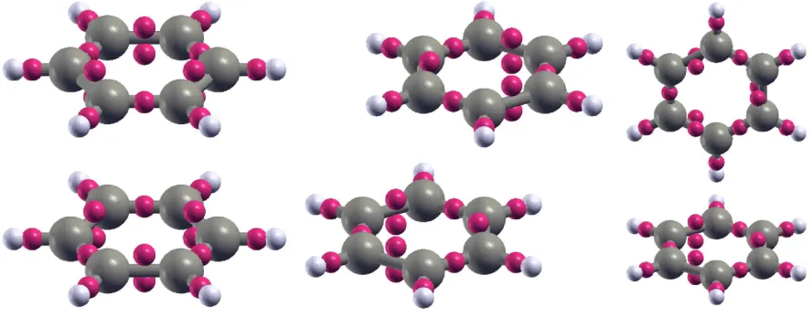
E. Benzene
For a benzene ring, the valence states are represented by 15 doubly-occupied Wannier functions. The MLWF optimization procedure in this case breaks the D6h symmetry of
Figure 6. Colours as in Fig. 4. Left: Ethene dimer with six MLWFs per molecule. Right: Ethene
dimer with seven MLWFs per molecule. The centres of thep-like MLWFs are placed on the carbon
atoms, but here we show the centres of the individual lobes of thesep-like orbitals as calculated by
our method.
3.5 4.0 4.5 5.0
Interdimer distance (Å) -2.0
-1.5 -1.0 -0.5 0.0
Binding energy (kcal/mol)
DFT-PBE
Semi-empirical DFT+D Silvestrelli (12 MLWFs) This work (14 MLWFs) CCSD(T)
Figure 7. Binding energy for an ethene dimer with various methods.
[image:15.595.191.417.396.555.2]Figure 8. The three configurations used for the benzene dimer calculations: S (vertical
displace-ment), PD (vertical and lateral displacement) and T (vertical displacement plus rotation in plane
of one molecule), and the valence MLWF centres in each case (depicted by pink spheres).
alignment is defined by where the initial guesses for the centres of the Wannier functions are placed.
The case of the benzene dimer therefore illustrates again the need to include the unoccu-pied antibonding states in the construction of the MLWFs: doing so increases the number of MLWFs and introduces partial occupancies, but restores theD6h symmetry of the system
and also localises the MLWFs more. This then makes the vdW contribution independent of the initial guess for the Wannier function centres.
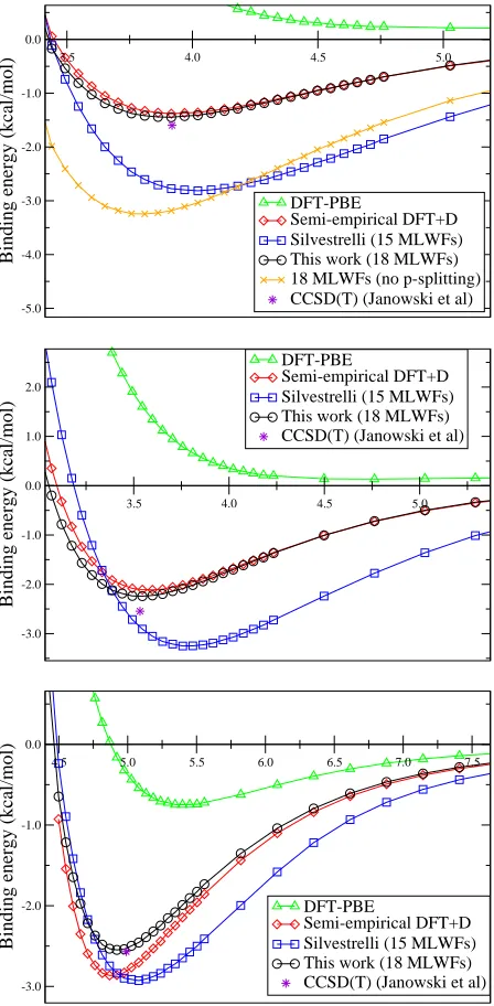
We applied our implementation of the original Silvestrelli’s method (with 15 MLWFs), and then our modified method (with 18 MLWFs, partial occupancies and splitting of p-like
states) to determine the binding energy as a function of displacement for three types of displacement (labelled S, PD, and T, illustrated in Fig. 8 of one of the molecules in the benzene dimer. We compare this to DFT+D and to the CCSD(T) calculations of Ref. 35. We note that we used the same bond lengths for C-C and C-H as Ref. 35 to within two decimal places, to construct perfectly symmetric benzene rings for our calculations.
The binding energy curves for the various methods for the three configurations are shown in Fig. 9.
3.5 4.0 4.5 5.0
Interdimer distance (Å) -5.0
-4.0 -3.0 -2.0 -1.0 0.0
Binding energy (kcal/mol)
DFT-PBE
Semi-empirical DFT+D Silvestrelli (15 MLWFs) This work (18 MLWFs) 18 MLWFs (no p-splitting) CCSD(T) (Janowski et al)
3.5 4.0 4.5 5.0
Interdimer distance (Å) -3.0
-2.0 -1.0 0.0 1.0 2.0
Binding energy (kcal/mol)
DFT-PBE
Semi-empirical DFT+D Silvestrelli (15 MLWFs) This work (18 MLWFs) CCSD(T) (Janowski et al)
4.5 5.0 5.5 6.0 6.5 7.0 7.5
Interdimer distance (Å) -3.0
-2.0 -1.0 0.0
Binding energy (kcal/mol)
DFT-PBE
[image:17.595.194.418.71.527.2]Semi-empirical DFT+D Silvestrelli (15 MLWFs) This work (18 MLWFs) CCSD(T) (Janowski et al)
Figure 9. Binding energy (kcal/mol) curves for the various methods for the benzene dimer in the
S, PD and T configurations (top, middle and bottom respectively). For the S configuration we also
show the curve using 18 MLWFs per molecule if no p-splitting is used; in this case the method
overbinds. CCSD(T) benchmark values are from Janowski et al.35
Silvestrelli’s method does not agree asymptotically with the DFT+D curve (red diamonds). In the T configuration Silvestrelli’s method performs better in terms of equilibrium distance, binding energy and asymptotics as it can be seen in Fig. 9 (bottom).
Method S PD T
Silvestrelli (15 MLWFs) 4.01 3.78 5.06
This work (18 MLWFs) 3.89 3.53 4.93
Semi-empirical DFT+D 3.93 3.58 4.89
[image:18.595.199.411.71.183.2]CCSD(T) (Janowskiet al35) 3.92 3.53 4.99
Table I. Equilibrium distances in Å for the benzene dimers in the three configurations (Fig. 8) using
the various methods. For all DFT calculations the PBE functional was used.
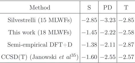
Method S PD T
Silvestrelli (15 MLWFs) −2.85 −3.23 −2.85
This work (18 MLWFs) −1.45 −2.22 −2.58
Semi-empirical DFT+D −1.38 −2.11 −2.87
CCSD(T) (Janowskiet al35) −1.60 −2.55 −2.57
Table II. Binding energies (kcal/mol) at equilibrium geometry for the benzene dimers in the three
configurations (Fig. 8) using the various methods. For all DFT calculations the PBE functional
was used.
p-like states is not used (orange crosses); it is clear that in this case the method does not
perform well, as replacing a p-like orbital by ans-orbital is a very poor approximation.
Our modified method (black circles in Fig. 9), on the other hand, has excellent agreement in terms of equilibrium distances and binding energies with the DFT+D curves and the CCSD(T) values, for all three configurations, to within 0.05 Å and 0.33 kcal/mol (Table I and II); the asymptotic behaviour of the energy is also better captured.
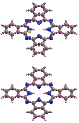
F. H2Pc and CuPc
[image:18.595.187.423.239.350.2]six-membered rings, representing delocalised π-bonds. We also find, however, that using
only the 93 valence MLWFs (186 valence electrons) is problematic, as a good representation of the electronic density of the system cannot be obtained in this way since this breaks the symmetry of the system, but most importantly it yields one lone MLWF of unrealistically large spread (∼2.5 Å) located some distance from any atoms (Fig. 10 (top)). This is due to the fact that an odd number (93 MLWFs) is incompatible with the D2h symmetry of the
molecule.
Using a larger and even number of MLWFs (112 per molecule) we can restore this D2h
symmetry of the molecule (Fig. 10 (bottom)) and represent the electronic density of the system in a way more compatible with its chemistry. When anti-bonding states are included, it is important to make a chemically intuitive initial guess for the centres and forms of the MLWFs. We make initial guesses as follows: we place p-like orbitals on the carbon atoms
and s-like orbitals on every bond andp-like orbitals on the hydrogenated nitrogens as well
as two s-like orbitals on every non-hydrogenated nitrogen atom. In this way, we have
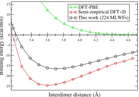
partly occupied MLWFs that represent the 372 valence electrons of the dimer. The binding energy curves obtained by using this representation and our modifications to Silvestrelli’s method are shown in Fig. 11 and compared to DFT+D. The binding energy obtained from our method is −16.55 kcal/mol and the equilibrium distance 3.70 Å; with DFT+D we obtain −18.91 kcal/mol and 3.68 Å. As for benzene, we see very good agreement with DFT+D; these values roughly agree with the stacking distance of crystalline H2Pc (around 3.2–3.4 Å)36. Silvestrelli’s original method severely overbinds the dimer (giving a binding energy of −41 kcal/mol) because of the unphysically large spread of the lone MLWF that appears in the valence representation. This is due to the strong dependence of the vdW energy on the spreads (Eq. (12)).
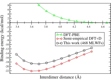
In the case of CuPc dimer (vertically displaced S configuration) we again do not use the valence manifold of 390 MLWFs per dimer (195 MLWFs per molecule: 98 spin up and 97 spin down), but instead use a larger manifold of MLWFs. We note that the dimer configuration used here does not correspond to any phases CuPc is observed in experimentally, but was used for illustrative purposes as it is the simplest one. This is a spin-polarized system, so a different set of MLWFs is required for spin up/down electrons, yielding a total of 234 singly occupied MLWFs per molecule (117 for every spin channel). There are 10 d-like MLWFs
Figure 10. Left: Phthalocyanine (H2Pc) molecule and its valence MLWF centres. Hydrogen atoms
are by small white spheres, carbon atoms by large grey spheres and nitrogen atoms by large blue
spheres. The MLWF centres are shown by the small pink spheres. Using only the valence MLWFs
does not give a satisfactory description of the system since it yields a lone MLWF of unphysically
large spread (shown by large yellow sphere and labelled by the letter L). Right: H2Pc molecule
and its 112 MLWF centres, now including anti-bonding states. With this representation all the
D2h symmetry of the ring is restored and a better chemical picture is given. There are s-like
orbitals on every bond and the non-hydrogenated nitrogens, and p-like partly occupied orbitals
on every carbon the two hydrogenated nitrogens (not shown here as these are located inside the
3.2 3.4 3.6 3.8 4.0 4.2 4.4 4.6
Interdimer distance (Å) -25
-20 -15 -10 -5 0 5 10 15
Binding energy (kcal/mol)
DFT-PBE
[image:21.595.196.418.70.225.2]Semi-empirical DFT+D This work (224 MLWFs)
Figure 11. Binding energy curves for H2Pc dimer in the S configuration (vertically displaced) versus
intermolecular distance obtained with the various methods.
nitrogens. The MLWFs corresponding to spin up and spin down electrons have essentially the same centres for the same bonds or atoms (Fig. 12).
In such cases, where some Wannier functions centres are very closely centred, it would be incorrect to consider them as separate fragments since this would violate the fundamental assumption of the ALL method, that it is valid for non-overlapping fragments only. This can be understood from the fact that Eq. (9) is strongly non-linear, so adding the contributions of overlapping density fragments does not give the same result as summing the densities be-forehand. As a result, Silvestrelli’s method severely overbinds the dimer (∼ −108kcal/mol), demonstrating that the method breaks down for overlapping fragments.
We alleviate this problem by amalgamating all the centres and spreads of the closely placed MLWFs (in this case the d-like MLWFs on Cu) into one MLWF with a centre and
spread given by the arithmetic mean of the closely placed MLWFs, and occupancies given by the sum of the separate MLWFs. The criterion for amalgamating MLWFs can be automated such that MLWFs less than a particular threshold distance apart are combined. In our case, we used a value of 0.1 Å for this threshold, which had the desired effect of including the
d-like orbitals on Cu in the amalgamation procedure, while leaving all other MLWFs in the
system unaffected.
Figure 12. Copper phthalocyanine (CuPc) molecule and its 234 MLWF centres, again including
anti-bonding states. Colours as in Fig. 10, with copper shown by the large brown sphere in the
centre. There are s-symmetry MLWFs on every bond and atom except for copper, p-like MLWFs
on the carbons and 5d-symmetry MLWFs on the copper atom. Now there are no p-like orbitals on
any nitrogen atom as for H2Pc.
3.4 3.6 3.8 4.0 4.2 4.4 4.6
Interdimer distance (Å) -22
-20 -18 -16 -14 -12 -10 -8 -6 -4 -2 0 2 4 6 8
Binding energy (kcal/mol)
DFT-PBE
Semi-empirical DFT+D This work (468 MLWFs)
Figure 13. Binding energy curves for the CuPc dimer in the S configuration (vertically displaced)
obtained using the various methods.
[image:22.595.194.416.410.571.2]G. Intermolecular C6 coefficients
It is expedient to define effective intermolecular C6 coefficients,
C6eff = 1 2
X
n,l
C6nl, (20)
where only intermolecular terms are summed over, i.e., n and l correspond to MLWFs
on different molecules, and the factor of 1/2 accounts for double-counting. In Table III, we compare our values to those of the original method of Silvestrelli, benchmark MP2 calculations and experimental results given in the database of Ref. 37.
As previously discussed in Ref. 2, comparison with experimental values is made somewhat difficult by the fact that they are obtained by fitting to experimental data and hence also include higher-order terms (C8, C10) in an effective manner.
Taking the experimental values as a benchmark, it can be seen from Table III that, for the systems under consideration, there is no clear or systematic improvement in calculated effective C6 coefficients with our modifications to Silvestrelli’s approach as compared to Silvestrelli’s original approach: in the case of ethene the original method compares more favourably, while in the case of the benzene dimers our approach performs much better. In spite of this, however, it is worth noting that our approach (as shown earlier) significantly improves the values obtained for equilibrium separations and binding energies, as compared to CCSD(T), for all systems considered for which we have access to CCSD(T) results.
H. Sensitivity to cutoff radius rc
The sensitivity of the binding energy on the cutoff radius rc in Eq. 12 was tested on the
S configuration of the benzene dimer with 18 MLWFs per molecule (Fig. 14). Even small changes of 1% in the cutoff radius result in significant changes in the binding energy curves, with the binding energy and equilibrium distance varying by 6-8% and 0.2-0.8% respectively. For larger changes in rc, the method breaks down, as the energy changes are unphysically
System C6 (Eha60)
Silvestrelli This work MP2 Experimental
Argon 92.7 - 76.1 64.3
Methane 99.1 - 119 130
Ethene 275 208 328 300
Benzene S 2727 1258 2364 1723
Benzene PD 2727 1257 2364 1723
[image:24.595.172.439.72.245.2] [image:24.595.191.418.376.537.2]Benzene T 2769 1232 2364 1723
Table III. Effective intermolecular C6 coefficients. MP2 and experimental values are drawn from
Ref. 37. For the argon and methane dimers, our approach is identical to the original method
of Silvestrelli. The differences between the values reported in the first column (Silvestrelli) and
those in Ref. 2 are attributable to the different calculational details such as choice of exchange and
correlation functional, simulation cell size and plane-wave energy cutoff.
3.40 3.60 3.80 4.00 4.20 4.40 4.60 4.80 5.00 Interdimer distance (Å)
-2.8 -2.6 -2.4 -2.2 -2.0 -1.8 -1.6 -1.4 -1.2 -1.0 -0.8 -0.6 -0.4 -0.2
Binding energy (kcal/mol)
0.90 rc 0.99 rc 1.00 rc 1.01 rc 1.10 rc
Figure 14. Binding energy curve for the benzene dimer in the S configuration for various values of
rc using our modified method with 18 MLWFs per molecule.
V. CONCLUSION
in-duced by considering only the valence manifold in the construction of the MLWFs, may introduce arbitary dependence on initial guesses in a way that significantly affect the vdW energy. We have shown that arbitrarily-broken symmetries may often be restored by in-creasing the number of Wannier functions used and generating them with a suitably-chosen range of the conduction states as well as the valence states. This necessitates the inclusion of occupancies in the formalism. We note that in cases where no symmetries are restored when we use more MLWFs, as in the example of ethene, it is the better localisation of the MLWFs that may be responsible for improved vdW energies, since the method is based on pairwise summation of well-separated fragments.
Particularly, in cases with a larger number of Wannier functions, we have shown that the approximation implicit in replacing the true Wannier functions with hydrogenic s-orbitals
may not always yield an accurate representation of the electronic denstiy, and have shown how in cases where there is p-like symmetry, it is better to substitute the p-symmetry
functions with two s-like functions. By considering the problems associated with applying
these adapted methods to larger systems such as H2Pc and CuPc, we have demonstrated that the approach is not necessarily a good candidate for studying larger systems, where specifying initial guesses for a large number of non-trivial MLWFs may be difficult; chemical insight for the form of these higher-lying states has to be employed, but becomes more difficult for even larger systems. In the case of copper phthalocyanine, we showed that MLWFs that are centred effectively at the same point (such as the five d-like MLWFs on
ACKNOWLEDGMENTS
The authors acknowledge the support of the Engineering and Physical Sciences Research Council (EPSRC Grant No. EP/G055882/1) for funding through the HPC Software Devel-opment program. The authors are grateful for the computing resources provided by Imperial College’s High Performance Computing service, which has enabled all the simulations pre-sented here.
REFERENCES
1P. L. Silvestrelli, Physical Review Letters 100, 053002 (2008).
2P. L. Silvestrelli, The Journal of Physical Chemistry A 113, 5224 (2009). 3P. Hohenberg and W. Kohn, Physical Review 136, B864 (1964).
4W. Kohn and L. J. Sham, Physical Review 140, A1133 (1965). 5E. Zaremba and W. Kohn, Physical Review B 13, 2270 (1976).
6B. I. Lundqvist, Y. Andersson, H. Shao, S. Chan, and D. C. Langreth, International Journal of Quantum Chemistry 56, 247 (1995).
7Y. Andersson, D. C. Langreth, and B. I. Lundqvist, Physical Review Letters 76, 102 (1996).
8J. F. Dobson and B. P. Dinte, Physical Review Letters 76, 1780 (1996).
9W. Kohn, Y. Meir, and D. E. Makarov, Physical Review Letters 80, 4153 (1998). 10J. F. Dobson and J. Wang, Physical Review Letters 82, 2123 (1999).
11H. Rydberg, B. I. Lundqvist, D. C. Langreth, and M. Dion, Physical Review B 62, 6997 (2000).
12M. Dion, H. Rydberg, E. Schröder, D. C. Langreth, and B. I. Lundqvist, Physical Review Letters 92, 246401 (2004).
13A. Tkatchenko and M. Scheffler, Physical Review Letters 102, 073005 (2009). 14P. L. Silvestrelli, Chemical Physics Letters 475, 285 (2009).
15P. L. Silvestrelli, F. Toigo, and F. Ancilotto, The Journal of Physical Chemistry C 113, 17124 (2009).
17P. L. Silvestrelli, K. Benyahia, S. Grubisiˆc, F. Ancilotto, and F. Toigo, The Journal of Chemical Physics 130, 074702 (2009).
18P. Giannozzi, S. Baroni, N. Bonini, M. Calandra, R. Car, C. Cavazzoni, D. Ceresoli, G. L. Chiarotti, M. Cococcioni, I. Dabo, A. D. Corso, S. de Gironcoli, S. Fabris, G. Fratesi, R. Gebauer, U. Gerstmann, C. Gougoussis, A. Kokalj, M. Lazzeri, L. Martin-Samos, N. Marzari, F. Mauri, R. Mazzarello, S. Paolini, A. Pasquarello, L. Paulatto, C. Sbrac-cia, S. Scandolo, G. Sclauzero, A. P. Seitsonen, A. Smogunov, P. Umari, and R. M. Wentzcovitch, Journal of Physics: Condensed Matter 21, 395502 (2009).
19X. Gonze, B. Amadon, P.-M. Anglade, J.-M. Beuken, F. Bottin, P. Boulanger, F. Bruneval, D. Caliste, R. Caracas, M. Côté, T. Deutsch, L. Genovese, P. Ghosez, M. Giantomassi, S. Goedecker, D. Hamann, P. Hermet, F. Jollet, G. Jomard, S. Leroux, M. Mancini, S. Mazevet, M. Oliveira, G. Onida, Y. Pouillon, T. Rangel, G.-M. Rignanese, D. Sangalli, R. Shaltaf, M. Torrent, M. Verstraete, G. Zerah, and J. Zwanziger, Computer Physics Communications 180, 2582 (2009).
20N. Marzari and D. Vanderbilt, Physical Review B 56, 12847 (1997). 21G. H. Wannier, Phys. Rev. 52, 191 (1937).
22K. S. Thygesen, L. B. Hansen, and K. W. Jacobsen, Phys. Rev. Lett. 94, 026405 (2005). 23K. S. Thygesen, L. B. Hansen, and K. W. Jacobsen, Phys. Rev. B 72, 125119 (2005). 24I. Souza, N. Marzari, and D. Vanderbilt, Physical Review B 65, 035109 (2001).
25A. A. Mostofi, J. R. Yates, Y. Lee, I. Souza, D. Vanderbilt, and N. Marzari, Computer Physics Communications 178, 685 (2008).
26S. Grimme, J. Antony, T. Schwabe, and C. Mück-Lichtenfeld, Organic & Biomolecular Chemistry 5, 741 (2007), PMID: 17315059.
27X. Wu, M. C. Vargas, S. Nayak, V. Lotrich, and G. Scoles, The Journal of Chemical Physics 115, 8748 (2001).
28M. Shelley, N. Poilvert, A. A. Mostofi, and N. Marzari, (2011), http://arxiv.org/abs/1101.3754.
29S. Grimme, Journal of Computational Chemistry 27, 1787 (2006).
30V. Barone, M. Casarin, D. Forrer, M. Pavone, M. Sambi, and A. Vittadini, Journal of Computational Chemistry 30, 934 (2009).
33P. Slaví˘cek, R. Kalus, P. Pa˘ska, I. Odvárková, P. Hobza, and A. Malijevský, The Journal of Chemical Physics 119, 2102 (2003).
34J. ˘Rezá˘c, P. Jure˘cka, K. E. Riley, J. ˘Cerný, H. Valdes, K. Pluhá˘ckovă, K. Berka, T. ˘Rezá˘c, M. Pito˘nák, J. Vondrá˘sek, and P. Hobza, Collect. Czech. Chem. Commun. 73, 1261 (2008).
35T. Janowski and P. Pulay, Chemical Physics Letters 447, 27 (2007).
36E. Orti and J. L. Bredas, The Journal of Chemical Physics 89, 1009 (1988).