Durham Research Online
Deposited in DRO:11 April 2018
Version of attached le: Accepted Version
Peer-review status of attached le: Peer-reviewed
Citation for published item:
Utkin, L.V. and Coolen, F.P.A. (2018) 'A robust weighted SVR-based software reliability growth model.', Reliability engineering and system safety., 176 . pp. 93-101.
Further information on publisher's website:
https://doi.org/10.1016/j.ress.2018.04.007
Publisher's copyright statement:
c
2018 This manuscript version is made available under the CC-BY-NC-ND 4.0 license
http://creativecommons.org/licenses/by-nc-nd/4.0/
Use policy
The full-text may be used and/or reproduced, and given to third parties in any format or medium, without prior permission or charge, for personal research or study, educational, or not-for-prot purposes provided that:
• a full bibliographic reference is made to the original source
• alinkis made to the metadata record in DRO
• the full-text is not changed in any way
The full-text must not be sold in any format or medium without the formal permission of the copyright holders. Please consult thefull DRO policyfor further details.
Durham University Library, Stockton Road, Durham DH1 3LY, United Kingdom Tel : +44 (0)191 334 3042 | Fax : +44 (0)191 334 2971
A robust weighted SVR-based software reliability growth model
Lev V. Utkin1, Frank P.A. Coolen2
1Telematics Department, Central Scientific Research Institute of Robotics and Technical Cybernetics,
Peter the Great Saint-Petersburg Polytechnic University, St. Petersburg, Russia
2Department of Mathematical Sciences, Durham University, United Kingdom
Abstract
This paper proposes a new software reliability growth model (SRGM), which can be re-garded as an extension of the non-parametric SRGMs using support vector regression to predict probability measures of time to software failure. The first novelty underlying the proposed model is the use of a set of weights instead of precise weights as done in the established non-parametric SRGMs, and to minimize the expected risk in the framework of robust decision making. The second novelty is the use of the intersection of two specific sets of weights, produced by the impreciseε-contaminated model and by pairwise comparisons, respectively. The sets are chosen in accordance to intuitive conceptions concerning the soft-ware reliability behaviour during a debugging process. The proposed model is illustrated using several real data sets and it is compared to the standard non-parametric SRGM.
Keywords: Imprecise contaminated model, pairwise comparisons, quadratic programming, software reliability growth model, support vector regression
1. INTRODUCTION
Software reliability is one of the most important factors in the software development process, which directly impacts on software quality. According to [1], software reliability is defined as the probability of failure-free software operation for a specified period of time in a specified environment. One of the methods for analyzing software reliability is to consider a software testing process, where defects of software are detected and removed. As a result, the software reliability tends to grow. Therefore, in order to estimate the software reliability by using information from the software testing process, many software reliability growth models (SRGMs) have been developed and successfully verified and applied in many software projects. As pointed out by several authors [2, 3, 4], most SRGMs can be divided into two large groups: parametric and non-parametric models.
Parametric SRGMs are generally based on assumptions about the behaviour of the software faults and failure processes, usually in the form of some statistical characteristics, for example, probability distributions of time between failures of the software. Depending on the initial data representation, parametric SRGMs can also be divided into the times-between-failures or time-dependent models and the nonhomogeneous Poisson process
(NH-PP) based models. The first type of models uses times between successive software failures during the testing or debugging period in order to predict some probability measures of time to the next software failure. One of the best known software reliability models is the Jelinski-Moranda model [5], which assumes that the elapsed time between failures is governed by the exponential probability distribution with a parameter (failure rate) that is proportional to the number of remaining faults in the software. The second type of models uses numbers of software failures observed in a given period of time in order to predict how many software failures will be observed in a time period after the debugging process. The best known parametric models of the second type are the NHPP based SRGMs. An example of the NHPP models is the well known Goel–Okumoto NHPP model [6], which assumes that the cumulative number of failures follows a Poisson process, such that the expected number of failures in a given time interval after time t is proportional to the expected number of undetected faults at time t. Since parametric SRGMs depend on a priori assumptions about the nature of software faults and the stochastic behaviour of the software failure process, they have quite different predictive performances across various projects [2, 7].
Non-parametric SRGMs utilize machine learning techniques including artificial neural networks, genetic programming and support vector machines (SVMs) to predict the soft-ware reliability. One of the important advantages of the models is that they usually do not use any prior assumptions and are based only on fault history data. Many non-parametric SRGMs have been proposed in the literature [2, 3, 7, 8, 9, 10, 11, 12, 13, 14, 15, 16, 17, 18, 19, 20, 21]. Contributions to this field are continuing, For example, Barghout [22] presented a new non-parametric model which is based on the idea of separation of concern between the long term trend in reliability growth and the local behaviour. Ramasamy and Lak-shmanan [23] proposed another non-parametric model applying an infinite testing effort function. Bal and Mohaparta [24] proposed a nonparametric method using radial basis function neural network for predicting software reliability. Some models using the machine learning framework have been considered and reviewed by other authors [25, 26, 27]. It should be noted that most so-called non-parametric SRGMs are not non-parametric in the strictest sense, because most models require some parameters to be assigned, for example, parameters of a kernel in SVMs. Nevertheless, we will use the term non-parametric for such models in order to distinguish them from models of the first type.
Among all learning techniques applied for constructing non-parametric SRGMs, we select for consideration SVMs [28, 29]. Since many SRGMs can be regarded as special cases of regression models, we consider a learning technique known as support vector regression (SVR), which is a modification or a special case of the SVM. Many available non-parametric SRGMs are based on SVR [7, 11, 18, 30].
Numerical results with many non-parametric SRGMs based on the SVR confirm the advantage of SVR [11]. However, although the SVR shows good learning performance and is suitable for generalizations, there are some limitations of its practical use. A main problem in many projects is that there may only be few test data available. In this case, the use of SVR for constructing a SRGM may lead to incorrect results. Moreover, tuning
parameters of learning algorithms are based on the procedure of cross-validation which divides the learning set into two subsets: training and testing. If there is only a small total data set, then this division leads to even smaller training sets which cannot be used to correctly construct the model. Incorrect results occurring in such a scenario as a result of the SVR, where the expected risk as an error measure for minimization is replaced by an approximation, are called the ‘empirical expected risk’. This can be regarded as a bound depending on the so-called VC dimension introduced by Vapnik [29]. The empirical expected risk causes problems for very small training data sets. A further problem of such models is that all failures during a debugging process are viewed as equivalent. In other words, the first failures discovered in the test process have identical impact on the software reliability prediction as the last failures discovered in the debugging process. However, failures discovered in the early part of the debugging process may well be characterized by “simple” errors in software, which arise due to inattention or carelessness of a programmer. Once such errors have been removed, remaining failures, both those discovered later in the debugging process and those that remain and hence may lead to failures after testing, are more likely to share common features. Furthermore, there may be an effect of data ageing due to possible substantial changes of software during debugging. We should also note that an assumption about independence of times to failure in the model may be violated [31] because the experience of testers with the specific software is likely to grow during the debugging process.
A possible way to overcoming the first problem mentioned above is by assuming a prob-ability distribution over the elements of the training set instead of the uniform distribution, and to use it in the optimization problem of minimizing the risk measure. However, the question arises how we can justify that a specific probability distribution is better than the uniform distribution which is used in the empirical risk measure. The second problem can be overcome by assigning different weights to elements of the training set. In particular, a simple way is to assign ranked weights, with small weights assigned to the first elements of the training set (corresponding to the the early stages of the debugging process) and larger weights assigned to the later elements (corresponding to the later stages of the debugging process). Of course, this leads to other natural questions about the validity of the assigned weights and how changes of weights may affect the reliability prediction.
Taking into account the above mentioned issues, we propose a new non-parametric SRGM based on the SVR. The main idea underlying the new SRGM is to replace precise weights assigned to the elements of training data by a set of weights produced by means of special rules. In other words, based on a small amount of training data, we construct a set of distributions. Then we can choose a single distribution from the set which maximizes the expected risk in accordance with the minimax strategy as commonly used in theories and methods for decision support. The chosen distribution, as well as the bounds of the set of distributions, depend on the unknown reliability model parameters which have to be computed. After substituting the “optimal” probability distribution into an expression for the expected risk, we can compute the optimal parameters of the regression model by minimizing the risk measure over the set of values of parameters. The properties of
normalized weights of elements are the same as those of probabilities, within the scope of the considered model. We will use the term ‘weights’ instead of ‘probabilities’.
Let us explain the selection of a single distribution from the set of distributions. In fact, by replacing the precise weights of training data with a set of weights, we equivalently replace the expected risk measure with a set of risk measures such that every measure corresponds to a weight distribution from the set of weights. If we take a convex and compact set of weights, then it is easy to prove that the set of risk measures as a set of expectations makes up a closed interval with some lower and upper bounds. This implies that we have to choose a point inside the interval of risk measures in order to minimize the corresponding risk measure and to get the SRGM parameters. That is why we apply the minimax or robust strategy as one of the strategies to deal with interval-valued functionals. According to the minimax strategy we select the upper bound of the interval for minimizing and for getting the model parameters. In other words, we maximize (the upper bound) the expected risk over the set of distributions in order to minimize this upper bound over the SRGM parameters.
Another important novel idea underlying the proposed SRGM is that we consider the intersection of two sets of weights. The first set is produced by the linear-vacuous mixture or imprecise ε-contaminated model [32], which can be viewed as a generalization of the well-known ε-contaminated (robust) model [33, Section 4.2.]. The application of this model relaxes the uniform distribution of weights, but does not assign a precise distribution. The second set is produced by a set of linear comparative equalities which softly rank the weights. We again do not assign precise weights for ranking the elements of training data. The second set allows us to relax the strict ranking. Crucially, both these sets compensate each other: the use of each set on its own would tend to lead to very imprecise predictions of the software reliability after the debugging process, but the logical use of the intersection of these sets leads to quite reasonable levels of imprecision.
Robust SVMs with sets of weights have been studied for classification problems [34, 35, 36]. Similar ideas as in those models are applied to the SVR in this paper, which is the basis for the proposed robust SRGM. The robustness stems from the statistical sense as a tool for taking into account how the SRGM behaves under a perturbation of the underlying statistical model, i.e., under changes of the uniform distribution of weights in the empirical risk measure. The idea to use sets of weights in the form of imprecise statistical models suggests as name for the proposed SRGM in this paper: IWSRGM (Imprecise Weight SRGM).
The paper is organized as follows. The statement of the non-parametric SRGMs in the framework of the SVR is given in Section 2. A weighted extension of the SVR is considered in the same section. The weighted SVR under the condition that weights of examples are only known to belong to a compact and convex set is studied in Section 3. Properties and extreme points of two sets of weights and their intersection are provided in Section 4. Section 5 presents an algorithm for the new model and its application to various real data sets, to illustrate the proposed IWSRGM and to compare it to the standard non-parametric SRGM. Some conclusions and future scope of the research are provided in Section 6.
2. WEIGHTED SVR AND THE NON-PARAMETRIC SRGM
We start by formulating the non-parametric SRGM in the general framework of predic-tive learning problems [28, 29, 37]. Parameters of the regression models are computed by minimizing a risk functional defined by a certain loss function and by a probability distri-bution of the noise. In regression analysis, we aim at estimating a functional dependency
f(x) between a set of sampled pointsX = (x1,x2, ...,xn) taken fromRm, and target values
Y = (y1, y2, ..., yn) with yi ∈R. In the framework of machine learning, the regression
prob-lem can be stated in the same way. We assume that there are n training data (examples)
S ={(x1, y1),(x2, y2), ...,(xn, yn)}, in which xi ∈ Rm represents a feature vector involving
m features and yi ∈ R is an output variable. Let us write the function f(x) in the form
f(x) = ha, φ(x)i+b, where a = (a1, ..., am), b are parameters of the function; φ(x) is a
feature map Rm → G such that the data points are mapped into an alternative higher-dimensional feature space G; h·,·i denotes the dot product. A learning machine has to choose the functionf(x) from a given set of functions, such that it optimally approximates the unknown dependency. This can be done in several ways, for example, by minimizing the empirical expected loss, where the loss function represents a measure of difference be-tween the estimate f and the actual value y given by the unknown function at a point x. The standard SVR technique is to assume that the probability distribution of the training points is the empirical (non-parametric) probability distribution function whose use leads to the empirical expected risk
Remp = 1 n n X i=1 l(yi, f(xi)).
Here l is the so-called -insensitive loss function with the parameter, which is defined as
l(y, f(x)) =
0, |y−f(x)| ≤,
|y−f(x)| −, otherwise.
Many realizations of the SVR use some distribution of weights w= (w1, ..., wn) instead
of the uniform distribution (1/n, ...,1/n) over the sampled pointsS in order to incorporate prior knowledge about importance of the points. The expected risk in this case is of the form: Rw = n X i=1 wil(yi, f(xi)). (1)
We assume here that the weights are non-negative and w1+...+wn= 1.
The parameters a and b are estimated by minimizing the following regularized risk function: RSVR,w = 1 2ha, ai+C n X i=1 wil(yi, f(xi)).
Here, the first term is the standard Tikhonov regularization or smoothness term [38];C >0 is the constant “cost” parameter which determines the trade-off between the flatness of f
and the amount up to which deviations larger than ε are tolerated [39].
Introducing slack variables ξi and ξi∗, the problem of minimizing the regularized risk
function can be written as follows: minimize 1 2ha, ai+C n X i=1 wi(ξi+ξi∗) (2) subject to ξi ≥0, ξi∗ ≥0, yi− ha, φ(x)i −b ≤+ξi, (3) ha, φ(x)i+b−yi ≤+ξ∗i. (4)
The above problem can be written in its dual formulation utilizing Lagrange multipliers
αi, α∗i, i= 1, ..., n, as [40] maximize n X i=1 yi(αi −α∗i)− n X i=1 (αi−α∗i) − 1 2 n X i,j=1 (αi−α∗i)(αj−αj∗)K(xi,xj), (5) subject to n X i=1 (αi−α∗i) = 0, (6) 0≤αi ≤Cwi, 0≤α∗i ≤Cwi, i= 1, ..., n. (7)
HereK(xi,xj) =hφ(xi), φ(xj)iis the kernel function, that is the inner product of the points
φ(xi) and φ(xj) mapped into the feature space. We do not need to compute the function
φ(x) explicitly due to the kernels, as it can be seen from the optimization problem that only the kernels are used in the objective function. Typical examples of kernel functions are linear, polynomial and Gaussian [41]. We will only use the Gaussian kernel, which is defined as
K(x,y) = exp − kx−yk2/σ2,
where σ is the kernel parameter determining the geometrical structure of the mapped samples in the kernel space. The regression functionf can now be written in terms of the Lagrange multipliers as f(x) = n X i=1 (αi−α∗i)K(x,xi) +b.
3. SVR WITH A SET OF WEIGHTS
Suppose that a weight vector, or distribution, belongs to a compact and convex set P, i.e., it is produced by finitely many linear constraints. Let us consider how to deal with this set of weights in the framework of the SVR.
First of all, we return to the expected risk (1). Since w ∈ P and the set P is convex, the corresponding set of RSVR,w is bounded by some lower and upper bounds for every set
of values of a and b. The upper bound determines the well-known minimax (pessimistic) strategy. According to the minimax strategy, a vectorwis selected from the setP such that the expected risk RSVR,w achieves its maximum RSVR,w for every fixed a and b. It should
be noted that the “optimal” vectorw may be different for different values of parameters a
and b. The minimax strategy can be explained in a simple way. We do not know a precise vector w and every vector from P can be selected. Therefore, we should take the “worst” distribution providing the largest value of the expected risk. The minimax criterion can be interpreted as an insurance against the worst case because it aims at minimizing the expected loss in the least favorable case [42]. This leads to the following optimization problem corresponding to the minimax strategy:
RSVR = min a,b maxw∈P C n X i=1 wil(yi, f(xi)) + 1 2ha, ai ! , (8) subject to (3), (4) and w∈ P.
Let us fix the valuesaandb. Then we have a linear programming problem with variables
w and constraints P. The set P is compact and convex. Therefore, the optimal solution can be found among the extreme points of the set. If the number of extreme points is s, then the above problem is reduced to s standard optimization problems of the form:
R(SVRk) = min a,b C n X i=1 w(ik)l(yi, f(xi)) + 1 2ha, ai ! , k= 1, ..., s, (9) subject to (3), (4).
Here w(ik) is the i-th element of the k-th extreme point. After solving s programming problems (9), we gets“local” solutionsa(k) andb(k),k= 1, ..., s. The final optimal solution of the problem corresponds to the largest objective function, i.e., we choose the parameters
a(k) and b(k) with k=k
opt such that
kopt = arg max
k=1,...,sR
(k) SVR.
It is interesting to note that extreme point w(kopt) is the “optimal” or “worst”
distri-bution providing the largest value of the expected risk. When we deal with the dual form (5)-(7), the same procedure is carried out, but we take the variables αi, αi∗, i = 1, ..., n,
The above approach for solving the optimization problem is very simple when we know the extreme points. Therefore, the next problem is to determine the extreme points of a suitable set P which is relevant and interesting for SRGMs.
4. WEIGHTS FOR OBSERVATIONS AND THEIR EXTREME POINTS
The main idea proposed in this paper, in order to improve the SRGM, is to consider two sets of weights. The first set is produced by the imprecise ε-contaminated model [32]. Its use relaxes the uniform distribution of weights. The second set is produced by a set of pairwise comparisons, which allows us to relax a strict ranking of weights in the sense that we do not assign precise weights for ranking the elements of the training data. The use of the first set of weights is a common way to robustify statistical models, particularly in case of a small number of training data. The second set of weights reflects the different importance of data obtained during the debugging process, where elements of the training set from the later stages of the debugging process are deemed to be more important than elements from the earlier stages of this process. There are several reasons why this is attractive. First, particularly simple errors in the software are likely to be removed early on in the debugging process. Secondly, there may be an effect of data ageing due to substantial change of the software during debugging: by removing errors, a programmer may change substantial parts of the software. Hence, software failure data from the earlier stages of the debugging process may be less relevant for predicting the software’s future reliability than data from the later stages, which can be reflected through the weights. Furthermore, the assumption about independence of times to failure may be violated. Cai et al. [31] pointed out that this assumption is not realistic in general, because test cases are usually not just selected at random but based on the previous experience with the software in the debugging process.
Both sets of weights discussed above are important for constructing the SRGM, so we aim at benefitting from the advantages of both sets. Therefore, we use the intersection of the sets to develop the new IWSRGM. This has the further important advantage that, while each of the two sets considered is rather large and would lead to overly pessimistic decisions based on the minimax criterion, these two sets compensate each other and their intersection reduces the size ofP substantially, making the minimax criterion more suitable in order to reach robust but realistic inferences. From the perspective of computation, it is important to note that both these sets of weights are convex, and the intersection of two convex sets is also a convex set which is totally defined by its extreme points. This implies that we can use the results obtained in the previous section in order to solve the programming problems (9) by determining the extreme points of the intersection of the two sets of weights. Next we present the two sets of weights in detail, followed by presentation of the intersection of these two sets.
4.1. The linear-vacuous mixture set of weights
The linear-vacuous mixture or impreciseε-contaminated models produce the setP(ε, w) of weights, or probabilities, w = (w1, ..., wn) such that wi = (1−ε)pi +εhi, where p =
(p1, ..., pn) is an elicited probability distribution, or the single probability distribution one
would expect to be most realistic, hi is arbitrary and h1+...+hn = 1, 0< ε <1. The set
P(ε, p) is a subset of the unit simplexS(1, n). Moreover, it coincides with the unit simplex when ε = 1. We denote the set P(ε, p) under condition p= (1/n, ...,1/n) as P(ε). It can be produced by n+ 1 hyperplanes
wi ≥(1−ε)n−1, i= 1, ..., n, w1+...+wn= 1. (10)
4.2. The set of weights produced by comparative information
Let us consider the following comparative information:
w1 ≤w2 ≤...≤wn, (11)
and the conditionw1+...+wn= 1.
A set M of weights w = (w1, ..., wn), which is produced by n−1 inequalities of the
form wi−wi−1 ≥0, n inequalities wi ≥0 and one equality w1 +...+wn = 1, has extreme
points of the form:
w1 w2 ... w3 w4 wn 0 0 ... 0 0 1 0 0 ... 0 1/2 1/2 0 0 ... 1/3 1/3 1/3 ... ... ... ... ... ... 1/n 1/n ... 1/n 1/n 1/n
It is interesting to see that the extreme points correspond to cases for which only several elements of the training data are used for constructing a regression model. Moreover, we have two extreme cases. The first one is the distribution of weights having only one non-zero element. In this case, the decision is made on the basis of the last point. Another extreme case coincides with the uniform distribution, as used for the empirical expected risk.
4.3. Intersection of the two sets of weights
Before we study the intersection of general sets P(ε) and M, we consider this inter-section for the case n = 3 by using the standard unit simplex. Figure 1 illustrates the unit simplex, every point of which is a possible weight vector (w1, w2, w3). The set M corresponds to the area restricted by the triangle ABC. The set P(ε) corresponds to the area restricted by the small simplex. Their intersection is restricted by the triangle BED
(the shaded area). We can see from the figure that the obtained set of weights is quite small when compared to the two individual sets of weights. Furthermore, the weights in the intersection, hence those used in the IWSRGM, are shifted towards the last (the third)
Figure 1: Intersection of the two sets of weights in the unit simplex forn= 3
vertex of the simplex, which means that the final element of the test data tends to get most weight. However, the simultaneous restriction to the small simplex corresponding to P(ε) prevents that the weight assigned to the last vertex becomes too large.
Now we turn our attention to the general case with n elements in the test data, for which the following proposition is crucial for computational feasibility of our proposed new model. The proof of this proposition is presented in the Appendix.
Proposition 1. The set of extreme points of the intersection P(ε) ∩ M consists of n elements of the form:
w1 =w2 =...=wi−1 = 1 n − ε n, wi =wi+1 =...=wn = 1 n + ε n · i−1 n−i+ 1, i= 1, ..., n.
Proposition 1 provides the set of the extreme points of the set P(ε)∩ M, which are necessary for solving the s = n programming problems (9). Every optimization problem is defined by one of the extreme points w(k), k = 1, ..., n. As a result, we have n standard weighted SVRs which can be easily solved.
Let us consider the set P(ε)∩ Min more detail as it is very interesting, and we believe it is attractive for a robust SRGM. Condition (11) produces a rather large set of weights
M and its sole use could lead to quite unlogical results. In particular, one of the extreme points ofMis (0, ...,0,1)., according to which the time to failure after the debugging process would be predicted on the basis of only the last observation from that process. It is therefore unlikely that one would want to use the entire set M to construct a robust SRGM. The set of weights P(ε) also has shortcomings. In particular, if we look at its extreme points,
then we observe that they consist of identical elements except for a single element which is larger than the other elements. In particular if ε is quite large, the prediction of the time to failure after the debugging process would be based substantially more on one of the elements of the test data than the other ones. The intersection of these sets P(ε) and M, however, avoids these problems and keeps attractive properties of both sets, in particular the fact that the weights are somewhat larger towards the data from the later stages of the debugging process but earlier data also keep some influence on the predictions. Finally, it is worth mentioning two special cases of the proposed IWSRGM. If ε = 0, then the set
P(ε)∩ M is reduced to the single point (1/n, ...,1/n), which corresponds to the standard SVR without considering sets of weights. The second extreme case occurs for ε= 1, which leads to P(1)∩ M=M, which means that only the set of weights reflecting the pairwise comparisons is used.
5. THE ALGORITHM FOR IWSRGM AND APPLICATIONS
In this section we present the algorithm for implementing the IWSRGM and we illustrate its application on six publicly available data sets. For each application, we randomly split the data set, consisting of n examples, into two subsets. One of these, the training set, is used to train (‘fit’) the model, while the subset of the remaining data, the test set consisting of ntest examples, is used to validate the model. For most data sets, we use about 20% of
examples for testing, so ntest is about equal to 0.2n, the randomly selected examples for
testing are given the indicesn−ntest+ 1, ..., n. Every regressor is computed by means of the
weighted SVR with parameter = 0 of the so-called -insensitive loss function, for details we refer to [39]).
Since the main purpose of these examples is to show the application of the IWSRGM on simple problems which are easy to visualize, the hyperparameters are chosen without fine tuning. For all performed experiments, we quantify the prediction performance with the normalized root mean square error measure (MSE), defined as
M SE = s Pntest i=1 (yi−f(xi))2 ntest .
Here yi and f(xi) are the actual value and the forecasted value for the time between
the (i−1)-th and i-th detected software failure, respectively. This MSE is only used to compare the application of different models to the same data set, hence it could also be defined with the denominator outside of the square-root, it would make no difference for these comparisons. The corresponding error measures for the standard and the IWSRGM algorithms will be denoted M SEst and M SEImp. We will also use the relative absolute difference between MSEs (RAMSE) which is defined as
RAM SE =|M SEst−M SEImp|/M SEst×100.
All experiments use a standard Gaussian radial basis function (RBF) kernel, with kernel parameter σ (see Section 2). Different values for the kernel parameter σ and the “cost”
parameter C have been tested and those leading to the best results have been used. This procedure is realized by considering all possible values ofσandC in a predefined grid. The grid for σ is determined as 2v, where v = −15, ...,0, ...,15. The values of C are taken in
accordance with the expression C0+iCs, whereC0 and Cs are experimentally determined
parameters, i= 1, ...,40.
Algorithm 1 describes the implementation of the IWSRGM in pseudo-code. The pro-posed IWSRGM has been evaluated and investigated using six publicly available data sets, taken from the literature, which all have different characteristics. The results are presented and discussed in the following subsections.
Algorithm 1The algorithm implementing the IWSRGM
Require: S (training set), parameters ε, , grid for σ ∈ {σ1, ..., σr}, grid for C ∈
{C1, ..., Ct}
Ensure: f(xn+1)
{Straining, Stesting}:S←Straining∪Stesting
i←1; j ←1
repeat
k ←1
repeat
w←w(k)
Solve problem (9) usingw, σi, Cj and Straining Compute R(SVRk) .
k+ +
until k > n
kopt(i, j)←arg maxk=1,...,nR
(k) SVR
M SE(i, j)←M SE(kopt(i, j), Stesting, σi, Cj, wkopt(i,j))
i+ +; j+ +
untili > r; j > t
(i, j)opt ←arg min(i,j)M SE(i, j)
f(xn+1)←
Pn
i=1(αi−αi∗)K(xn+1,xi) +b
5.1. Data Set 1
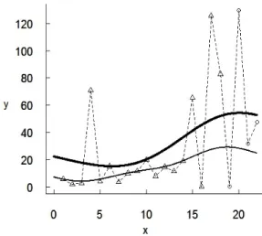
The first data set contains software inter-failure times taken from a telemetry network system by AT&T Bell Laboratories [43]. The data set contains 22 observations of the actual time series. The system receives and transmits data from a telemetry network which consists of telemetry events such as alarms, facility-performance information and diagnostic messages to operators for action. To test the system, system testers executed in a manner that emulated its expected use by system operators and other personnel. The system was tested for three months until it was released to the beta site. After this, data was collected for approximately another three months during beta-test execution [43, 44].
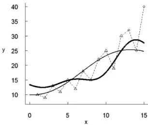
Figure 2: Fault detection prediction results with two SRGMs for Data Set 1
Figure 2 presents the fault detection prediction results based on two SRGMs: the standard non-parametric SRGM based on the SVR (the thin curve) and the IWSRGM (the thick curve), for which ε= 0.6 is used. The actual observations are also given (linked by the dashed curve), where the training data are depicted by triangles and the testing data by circles. It seems that the actual data have substantial heteroscedasticity, i.e., changes of variance, in particular after the 15-th failure detection. In such a scenario, it seems reasonable to base predictions more strongly on the observations from the later part of the training set than from the earlier part, as achieved by our method.
Figure 2 shows that the thin curve is close to most training points, especially at the beginning of the debugging process. However, it behaves unsatisfactory for the testing period, where the large variation of times to failure is observed. At the same time, the thick curve is more influenced by ‘anomalous’ points, which happens due to two reasons. First, the imprecise ε-contaminated model assigns larger weights to anomalous points because they increase the expected risk measure. Secondly, the set of weights produced by the comparative information assigns smaller weights to points at the beginning of the debugging process. The IWSRGM combines these two effects and performs better than the standard non-parametric SRGM for the testing set.
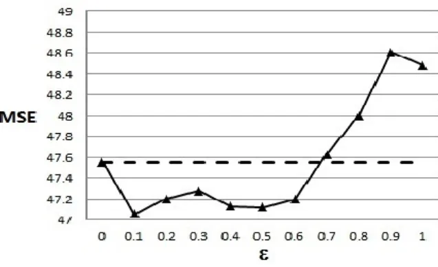
To get more insight into the proposed IWSRGM, we investigate how the prediction performance depends on the contamination parameter ε, by considering values at steps 0.1 over the whole range 0 to 1 for ε. Note that ε = 0 corresponds to the standard non-parametric SRGM based on the SVR, as also used in Figure 2. Dependence of the MSE on the parameter ε is shown in Figure 3. The solid curve corresponds to the MSE obtained by using the proposed IWSRGM. The dashed line shows the MSE for ε = 0, i.e., for the standard non-parametric SRGM. It should be noted that the solid curves and dashed lines in the similar figures for all later data sets, in the following subsections, will denote the
Figure 3: Dependence of the MSE on the parameterε, Data Set 1
MSEs for the IWSRGM and the standard SRGM, respectively. Figure 3 shows that the MSE of the IWSRGM is smaller than the MSE of the standard model forε ≤0.6. Moreover, of the values considered, ε= 0.1 is optimal as it leads to the largest reduction of MSEs for the IWSRGM compared to the standard SRGM.
5.2. Data Set 2
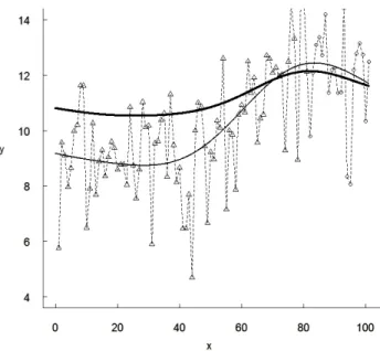
A further example of fault detection prediction results is shown in Figure 4, using data from a software inter-failure times series from [44], containing 101 observations. The two SRGMs and the actual data are represented in the same manner as in Figure 2. The observations are characterized by large variation. As a consequence, the influence of the parameterεon the MSE (see Figure 5) is quite weak: the largest RAMSE, at pointε= 0.7, is very small and equal to 1.7%.
5.3. Data Set 3
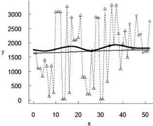
The next example uses data on helicopter main rotor blade part code, based on a system database collected from October 1995 to September 1999, as given in [45, Subsection 3.3.3]. The data set consists of 52 observations. The results are shown in Figure 6. This shows that variation of times to failure is rather large. Moreover, the reliability growth is almost invisible. At first glance, the predicted results of the two models (standard SRGM and IWSRGM) are close, due to the large training set. However, we can see from Figure 7, which shows the dependence of the MSE on the parameter ε, that the largest RAMSE is 15.6%, hence the IWSRGM provides a considerable improvement compared to the standard SRGM.
Figure 7 also shows that the MSE of IWSRGM is smaller than the MSE of the standard model for all ε. Some variation of the MSE as function of ε is caused by the small number of testing data. It is important to point out that the set M of comparative information itself (the case ε= 1) provides substantially better results than the standard model.
Figure 4: Fault detection prediction results with two SRGMs for Data Set 2
Figure 6: Fault detection prediction results with two SRGMs for Data Set 3
Figure 8: Fault detection prediction results with two SRGMs for Data Set 4
Figure 9: Dependence of the MSE on the parameterε, Data Set 4
5.4. Data Set 4
Next we show an example using data from testing an on-line data entry software package developed at IBM [46]. The data set contains 15 observations. The results are presented in Figure 8. This is only a small data set, but there is clear reliability growth. Figure 9 illustrates how the MSE depends on the parameter ε, it shows that the introduction of the set of weights together with the use of the minimax strategy, in our newly proposed method, leads to better results. The optimal value of ε = 0.4 as this corresponds to the largest difference between the MSEs of the standard SRGM and the IWSRGM; the largest RAMSE is 6.3%.
5.5. Data Set 5
Next we consider the NTDS failure data set, first reported in [5] and containing 34 failure data. The data set can be also found in [45, Subsection 4.8]. The results are shown
Figure 10: Fault detection prediction results with two SRGMs for Data Set 5
Figure 11: Dependence of the MSE on the parameterε, Data Set 5
in Figure 10. For most of the debugging period, the data do not indicate reliability growth, we even observe some reduction of reliability. Only in the later stages of the debugging period the data show reliability growth. It should also be noted that the observed data show considerable heteroscedasticity. Therefore, this is another illustrative example when sets of weights may lead to better results, in particular the use of the set M of pairwise comparisons. This is indeed the case as can be seen from Figure 11). The largest RAMSE is 15.2%, so the IWSRGM performs considerably better than the standard SRGM.
5.6. Data Set 6
As final example, we show a case in which the incorporation of the weighted sets does not improve the standard SRGM. We use the software inter-failure time series reported in [47] and evaluated in [48] (‘JDM-I failure data’). The data set contains 17 observations.
Figure 12: Fault detection prediction results with two SRGMs for Data Set 6
Figure 13: Dependence of the MSE on the parameterε, Data Set 6
The results are shown in Figure 12. The same examples were obtained for different values of ε. Here curves corresponding to the different SRGMs are very close to each other. Moreover, we can observe some reduction of the software reliability during the debugging process. Figure 13 shows that the standard SRGM is better that the IWSRGM, but only marginally so as the largest RAMSE is 0.9%. Of course, ε = 0 reduces the IWSRGM to the standard SRGM, so a search in the newly proposed model over the different values for
ε will indicate that the special case of the standard SRGM performs best for these data.
6. Concluding remarks
In this paper we have presented a new software reliability growth model (SRGM), called Imprecise Weight SRGM (IWSRGM), which can be viewed as an extension of the standard non-parametric SRGMs using the SVR to predict probability measures of time to the next
software failure. Two main ideas led to the proposed model. The first one is to use the set of weights instead of precise ones and to minimize the expected risk in the framework of minimax (hence ‘pessimistic’) decision making. The second idea is to use the intersection of two specific sets of weights, which are chosen in accordance with some intuitive conceptions concerning the software reliability behaviour during a debugging process.
The IWSRGM is attractive from both the computation and development points of view, due to the representation of the complex optimization problem (8) by a finite set of standard quadratic programmes which implement the SVR. This representation requires knowledge of the extreme points of the set of weights used for constructing the model, which was presented in this paper. This also implies that variations to the proposed IWSRGM can be derived by using other sets of weights, as long as these sets are compact, convex and their extreme points are known. This suggests an interesting topic for future research, namely to construct different sets of weights corresponding to different software reliability growth scenarios.
Six examples with data sets from the literature have been presented. These have il-lustrated that the proposed IWSRGM tends to perform better than the standard non-parametric SRGM, although it is possible that no improvement may be achieved (Data Set 6). At the same time, we have observed that the quality of predictions depends on the parameter ε of the linear-vacuous mixture or imprecise ε-contaminated model, whose optimal value is a priori unknown. It can be obtained only by considering all possible values in a predefined grid. These examples have shown that the proposed model may provide worse results in comparison with the standard non-parametric SRGM for some values of
ε, especially for large values when the set of weights produced by pairwise comparisons becomes prevailing over the set produced by the imprecise ε-contaminated model.
This new model, like other software reliability growth models, can be used to provide insight into the improvement of the software during a testing and debugging process. It should be noted that only the times-between-failures models for software reliability growth have been studied in the paper. However, we do not foresee major difficulties in extending the proposed approach to the NHPP-based SRGMs, this is left as a topic for future research. Another direction for future research is incorporation of prior statistical knowledge into the SRGM, which may improve the predictive properties of the developed models.
Appendix: Proof of Proposition 1
Denote the set of inequalities (10) by P and the set of inequalities (11) by M. We do not include into P inequalities wi ≥0 because all points with wi = 0 for at least one i do
not belong to the intersection P(ε)∩ M. Let us consider the system of 2n−1 inequalities fromP and M. It is know that every extreme point satisfiesn−1 equalities fromP ∩M. We study the following cases.
Case 2. n−2 equalities are from P, and 1 constraint is from M. This implies that there is one strict inequalitywi−1 < wi fromP and one equality wk =n−1−εn−1 fromM. Here
we have to consider two subcases. The first subcase is k ≥i. Then
wi−1 < wi =wk=n−1−εn−1.
However, wi =wi+1 =... =wn. Hence, w1+...+wn = 1−ε < 1 and we have reached a
contradiction. Therefore, this subcase does not give extreme points. The second subcase is k < i. Then
w1 =w2 =...=wi−1 = 1
n − ε n.
Then there holds
wi+...+wn= 1− n−1−εn−1 i. Hence, we get wi = 1−(n−1−εn−1)i n−i+ 1 = 1 n + ε n · i−1 n−i+ 1.
This is an extreme point for a fixedi. Note that the extreme point obtained in Case 1 can be regarded as a special case of Case 2 when i= 1.
Case 3. n−3 equalities are fromP, and 2 constraints are fromM. This implies that there are two strict inequalities wi−1 < wi and wj−1 < wj, i < j, from P, and two equalities
wk = n−1 −εn−1 and wl = n−1 −εn−1, k < l. The subcase with k ≥ i or l ≥ i is not
considered here, it leads to a contradiction similar to first subcase in Case 2. Hence we can restrict attention to the second subcase with k < i and l < i. Then we can write
w1 =w2 =...=wi−1 = 1
n − ε n.
Suppose that ws =a, s=i, ..., j−1, and ws =b, s=j, ..., n, i.e.,
wi =...=wj−1 =a, wj =...=wn=b.
Here due to inequalitieswi−1 < wi and wj−1 < wj, we can write
1
n − ε
n < a < b.
The numbers a and b satisfy the following obvious condition:
1 n − ε n (i−1) +a(j −i) +b(n−j+ 1) = 1.
It can be seen that there are infinitely many values ofaandbsatisfying the above condition. This implies that we get an edge of the corresponding polytope. The same can be obtained, in similar manner, for the other cases where we take n−r equalities from P, and r−1 constraints from M. Consequently, Case 2 totally defines all extreme points, as was to be proved.
Acknowledgements
The authors are grateful for useful comments by three reviewers which led to improved presentation and suggested further topics for future related research.
References
[1] Lyu, M.R. (1996). Handbook of Software Reliability Engineering. McGraw-Hill, New York.
[2] Li, H.F., Lu, M.Y., Zeng, M., Huang, B.Q. (2012) A non-parametric software reliability modeling approach by using gene expression programming. Journal of Information Science and Engineering, 28, 1145–1160.
[3] Hua, Q.P., Xie, M., Ng, S.H., Levitin, G. (2007). Robust recurrent neural network modeling for software fault detection and correction prediction. Reliability Engineering and System Safety, 92, 332–340.
[4] Roy, P., Mahapatra, G.S., Rani, P., Pandey, S.K., Dey, K.N. (2014). Robust feedfor-ward and recurrent neural network based dynamic weighted combination models for software reliability prediction. Applied Soft Computing, 22, 629–637.
[5] Jelinski, Z., Moranda, P.B. (1972). Software reliability research. In: W. Greiberger, editor, Statistical Computer Performance Evaluation, pp 464–484. Academic Press, New York.
[6] Goel, A.L., Okomoto, K. (1979). Time dependent error detection rate model for software reliability and other performance measures. IEEE Transactions in Reliability, R-28, 206–211.
[7] Tian, L., Noore, A. (2005). Dynamic software reliability prediction: an approach based on support vector machines. International Journal of Reliability, Quality and Safety Engineering, 12, 309–321.
[8] Amina, A., Grunskeb, L., Colman, A. (2013). An approach to software reliability prediction based on time series modeling. The Journal of Systems and Software, 86, 1923–1932.
[9] Cai, K.Y., Cai, L., Wang, W.D., Yu, Z.Y., Zhang, D. (2001). On the neural network approach in software reliability modeling. The Journal of Systems and Software, 58, 47–62.
[10] Chiu, K.C., Huang, Y.S., Lee, T.Z. (2008). A study of software reliability growth from the perspective of learning effects. Reliability Engineering & System Safety, 93, 1410–1421.
[11] Jin, C., Jin, S.W. (2014). Software reliability prediction model based on support vector regression with improved estimation of distribution algorithms. Applied Soft Computing, 15, 113–120.
[12] Kim, T., Lee, K., Baik, J. (2015). An effective approach to estimating the parameters of software reliability growth models using a real-valued genetic algorithm. Journal of Systems and Software, 102, 134–144.
[13] Kumar, N., Banerjee, S. (2015). Measuring software reliability: A trend using machine learning techniques. In: Q. Zhu and A.T. Azar, editors, Complex System Modelling and Control Through Intelligent Soft Computations, volume 319 ofStudies in Fuzziness and Soft Computing, pp 807–829. Springer, Berlin.
[14] Kumar, P., Singh, Y. (2012). An empirical study of software reliability prediction using machine learning techniques. International Journal of System Assurance Engineering and Management, 3, 194–208.
[15] Li, H.F., Zeng, M., Lu, M.Y., Hu, X., Li, Z. (2012). Adaboosting-based dynamic weighted combination of software reliability growth models. Quality and Reliability Engineering International, 28, 67–84.
[16] Lou, J., Jiang, J., Shuai, C., Wu, Y. (2010). A study on software reliability prediction based on transduction inference. In: Test Symposium (ATS), 2010, 19th IEEE Asian, pp 77–80, Shanghai.
[17] Lou, J., Jiang, J., Shen, Q., Shen, Z., Wang, Z., Wang, R. (2016). Software reliability prediction via relevance vector regression. Neurocomputing, 186, 66–73.
[18] Moura, M.d.C., Zio, E., Lins, I.D., Droguett, E. (2011). Failure and reliability predic-tion by support vector machines regression of time series data. Reliability Engineering and System Safety, 96, 1527–1534.
[19] Pai, P.F., Hong, W.C. (2006). Software reliability forecasting by support vector ma-chines with simulated annealing algorithms. Journal of Systems and Software, 79, 747–755.
[20] Xing, F., Guo, P., Lyu, M.R. (2005). A novel method for early software quality predic-tion based on support vector machine. In: Proceedings of the 16th IEEE International Symposium on Software Reliability Engineering (ISSRE 2005), pp 1–10.
[21] Yang, B., Li, X., Xie, M., Tan, F. (2010). A generic data-driven software reliability model with model mining technique. Reliability Engineering and System Safety, 95, 671–678.
[22] Barghout, M. (2016). A two-stage non-parametric software reliability model.
Communications in Statistics - Simulation and Computation. Early online version: doi:10.1080/03610918.2016.1189567.
[23] Ramasamy, S., Lakshmanan, I. (2017) Machine learning approach for software relia-bility growth modeling with infinite testing effort function. Mathematical Problems in Engineering, Article ID 8040346, 6 pages. doi:10.1155/2017/8040346.
[24] Bal, P.R., Mohapatra, D.P. (2017). Software reliability prediction based on radial basis function neural network. In: Advances in Computational Intelligence, Sahana, S., Saha, S. (Eds). Advances in Intelligent Systems and Computing, vol 509. Springer, Singapore. pp.101-110.
[25] Algargoor, R.G., Saleem, N.N. (2013). Software reliability prediction using artificial techniques. International Journal of Computer Science Issues, 10, 274–281.
[26] Begum, M., Dohi, T. (2017). A neuro-based software fault prediction with Box-Cox power transformation. Journal of Software Engineering and Applications, 10, 288–309. [27] Choudhary, A., Baghel, A.S., Sangwan, O.P. (2016). Software reliability prediction modeling: A comparison of parametric and non-parametric modeling. In: Proceedings of the 6th International Conference - Cloud System and Big Data Engineering, pp 649–653.
[28] Hastie, T., Tibshirani, R., Friedman, J. (2001). The Elements of Statistical Learning: Data Mining, Inference and Prediction. Springer, New York.
[29] Vapnik, V. (1998). Statistical Learning Theory. Wiley, New York.
[30] Xing, F., Guo, P. (2005). Support vector regression for software reliability growth modeling and prediction. In: Advances in Neural Networks – ISNN 2005, volume 3496 of Lecture Notes in Computer Science, pp 925–930. Springer, Berlin.
[31] Cai, K.Y,, Wen, C.Y., Zhang, M.L. (1991). A critical review on software reliability modeling. Reliability Engineering and System Safety, 32, 357–371.
[32] Walley, P. (1991). Statistical Reasoning with Imprecise Probabilities. Chapman and Hall, London.
[33] Huber, P.J. (1981). Robust Statistics. Wiley, New York.
[34] Utkin, L.V., Zhuk, Y.A. (2014). Robust novelty detection in the framework of a contamination neighbourhood. International Journal of Intelligent Information and Database Systems, 7, 205–224.
[35] Utkin, L.V., Zhuk, Y.A. (2014). Imprecise prior knowledge incorporating into one-class classification. Knowledge and Information Systems, 41, 53–76.
[36] Utkin, L.V. (2014). A framework for imprecise robust one-class classification models.
International Journal of Machine Learning and Cybernetics, 5, 379–393.
[37] Vapnik, V. (1995). The Nature of Statistical Learning Theory. Springer, New York. [38] Tikhonov, A.N., Arsenin, V.Y. (1977). Solution of Ill-Posed Problems. W.H. Winston,
Washington DC.
[39] Smola, A.J., Scholkopf, B. (2004). A tutorial on support vector regression. Statistics and Computing, 14, 199–222.
[40] Tay, F.E.H., Cao, L.J. (2002). Modified support vector machines in financial time series forecasting. Neurocomputing, 48, 847–861.
[41] Scholkopf, B., Smola, A.J. (2002). Learning with Kernels: Support Vector Machines, Regularization, Optimization, and Beyond. MIT Press, Cambridge, Massachusetts. [42] Robert, C.P. (1994). The Bayesian Choice. Springer, New York.
[43] Pham, L., Pham, H. (2000). Software reliability models with time-dependent hazard function based on Bayesian approach. IEEE Transactions on Systems, Man, and Cybernetics, Part A, 30, 25–35.
[44] Pham, L., Pham, H. (2001). A Bayesian predictive software reliability model with pseudo-failures. IEEE Transactions on Systems, Man, and Cybernetics, Part A, 31, 233–238.
[45] Pham, H. (2006). System Software Reliability. Springer, London.
[46] Ohba, M. (1984). Software reliability analysis models. IBM Journal of Research and Development, 28, 428–443.
[47] Musa, J.D., Iannino, A., Okumoto, K. (1987). Software Reliability: Mesurement, Prediction, Application. McGraw-Hill, New York.
[48] Liu, J., Xu, M. (2011). Function based nonlinear least squares and application to Jelinski–Moranda software reliability model. Preprint arXiv:1108.5185.