IMT School for Advanced Studies, Lucca
Lucca, Italy
Graph–based techniques and spectral graph
theory in control and machine learning
PhD Program in Institutes, Markets and Technologies
Track in Computer, Decision and Systems Science
Curriculum in Control Systems
XXVIII Cycle
By
Rita Morisi
2016
The dissertation of Rita Morisi is approved.
Supervisor: Prof. Giorgio Gnecco, IMT School for Advanced Studies, Lucca
The dissertation of Rita Morisi has been reviewed by:
Prof. Franco Scarselli, Department of Information Engineering, Univer-sity of Siena
Prof. Vˇera K ˚urková, Department of Theoretical Computer Science, Academy of Sciences of the Czech Republic
IMT School for Advanced Studies, Lucca
2016
Contents
List of Figures x
List of Tables xv
Vita and Publications xviii
Abstract xxi
I
Introduction and background
1
1 Introduction 2
1.1 Graphs versatility and applications . . . 2
1.2 Problem statement . . . 4
1.3 Challenges and scientific contributions . . . 6
2 Introduction to graphs and spectral properties 9 2.1 Introduction . . . 9
2.2 Graph representation . . . 10
2.2.1 Graphs features and fundamental notions . . . 11
2.3 Spectral graph theory . . . 15
2.3.1 Spectral clustering technique . . . 17
2.3.2 Spectral clustering points of view . . . 18
2.3.3 Laplacian eigenvalues and their properties . . . 21
2.4 Summary . . . 22
II
The consensus problem and its graph of
intercon-nections
23
3 The consensus problem and its sparse variations 24 3.1 Introduction . . . 243.2 Consensus problem - the model . . . 25
3.2.1 Spectral properties of matrix P . . . 26
3.3 The Fastest Mixing Markov Chain Problem . . . 29
3.4 Sparse variations of the Fastest Mixing Markov – Chain problem . . . 31
3.4.1 Sparse variations of Problem FMMC - models . . . 32
3.4.2 Theoretical results for Problems FMMC-l1(η) and FMMCconstr-l1(η) . . . 34
3.4.3 Theoretical results for Problem FMMC-l0(η) . . . . 43
3.5 Results and Discussion . . . 52
3.5.1 Comparison of Problems FMMC-l1(η) and FMMC-l0(η) . . . 53
3.5.2 Comparison of Problems FMMC-l1(η), FMMCconstr-l1(η), and FMMC . . . 57
3.5.3 Discussion and Conclusions . . . 61
3.6 Summary . . . 62
4 Spectral graph theory in the consensus problem 64 4.1 Introduction . . . 64
4.2 Problem formulation . . . 65
4.2.1 Computation of the transition probability matrix . . 67
4.3 Dividing graphGto increase the convergence rate to the consensus state . . . 68
4.3.1 Spectral clustering . . . 70
4.3.2 Nearest supernode approach . . . 71
4.4 Consensus on the subgraphs and on the auxiliary graph . 74 4.4.1 Approximation of the global consensus state through the hierarchical method . . . 75
4.4.2 Definitions of the vectors of initial opinions, and asymptotic analysis . . . 78
4.4.3 Performance analysis . . . 80
4.5 Numerical examples and results . . . 82
4.5.1 Random geometric graph . . . 84
4.5.2 Planted partition graph . . . 87
4.5.3 Preferential Attachment model . . . 90
4.6 Drawbacks and refinements of the basic version of the method 92 4.6.1 Theantenna effect . . . 94
4.6.2 Numerical examples related to theantenna effect . . 98
4.6.3 A solution to overcome theantenna effect . . . 103
4.6.4 Choice of the supernodes in the planted partition model . . . 105
4.7 Discussion and Conclusions . . . 107
4.8 Summary . . . 109
III
Graphs in semi–supervised learning and in
model-ing data for features extraction
110
5 Graphs in semi-supervised learning 111 5.1 Introduction . . . 1115.2 Semi–supervised learning: a brief overview . . . 112
5.2.1 Manifold regularization . . . 113
5.3 Supervised and Semi-Supervised Classifiers for the Detec-tion of Flood-Prone Areas . . . 114
5.3.1 Flood–Prone Areas Dataset and Features . . . 117
5.3.2 Classification tasks and experimental settings . . . 118
5.4 The proposed learning approach . . . 119
5.5 Results and Discussion . . . 126
5.5.1 Experimental results . . . 126
5.5.2 Discussion and Conclusions . . . 134
5.6 Summary . . . 137
6 Graph-based features extraction in a supervised learning con-text 138 6.1 Introduction . . . 138
6.2 Degenerative Parkinsonisms - overview . . . 140
6.3 Patients and Methods . . . 141
6.3.1 Dataset preprocessing . . . 142
6.3.2 MR Imaging . . . 142
6.4 Pattern Recognition Analysis . . . 144
6.4.1 Modeling the dataset with graphs . . . 144
6.4.2 Classification model . . . 146
6.4.3 Feature selection . . . 149
6.5 Results and Discussion . . . 151
6.5.1 Binary and multi–class classification results . . . 151
6.5.2 Discussion and Conclusions . . . 159
6.6 Summary . . . 163
7 Conclusions 164 7.1 Concluding remarks . . . 164
7.2 Future directions . . . 166
A Support Vector Machines 169
B Laplacian Support Vector Machines 172
C Additional studies of the Cheeger’s inequality 174
List of Figures
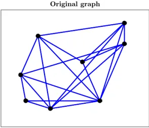
1 A toy example modeled by a graph with8vertices and20
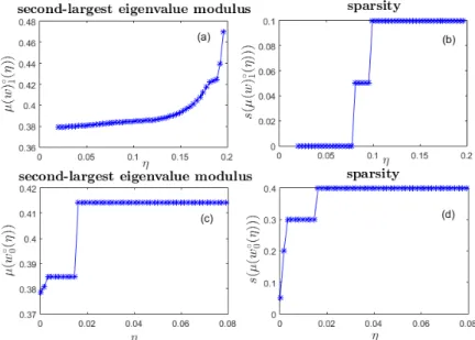
non self–loop edges. . . 54 2 Dependence on the regularization parameter of the
second-largest eigenvalue modulusµand the sparsitysfor the op-timal solutions of Problems FMMC-l1(η) (subplots (a) and
(b)) and FMMC-l0(η) (subplots (c) and (d)). . . 55
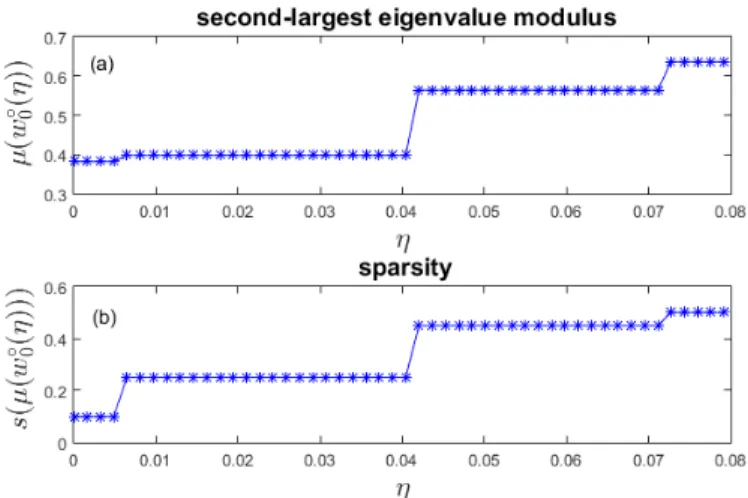
3 Dependence on the regularization parameter of the second-largest eigenvalue modulus µ and the sparsitys for the suboptimal solution of Problem FMMC-l0(η), obtained when
100subgraphs are randomly extracted from the whole set of connected non isomorphic subgraphs. . . 57 4 Dependence on the regularization parameter of the
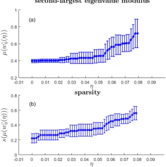
aver-age (over 10 trials) of the second-largest eigenvalue mod-ulusµ(upper plot) and of the sparsitys(lower plot) for the suboptimal solution of Problem FMMC-l0(η), obtained
when100subgraphs are randomly extracted from the whole set of connected non isomorphic subgraphs. . . 58
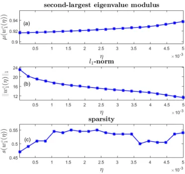
5 Dependence onηof the second–largest eigenvalue modu-lus of the weighted adjacency matrixP, thel1–norm and
the sparsity of an optimal solution of Problem FMMC–l1. . 59
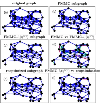
6 A comparison of the subgraphs associated with non-zero weights in the optimal solutions to Problems FMMC and FMMC-l1(η(j
◦)
). See the main text for explanations about the colors used in the figure. . . 60 7 A comparison of the subgraphs associated with non-zero
weights in the optimal solutions to Problems FMMC-l1(η(j
◦) ) and FMMCconstr-l1(η(j
◦)
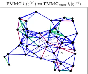
). This is obtained by merging such subgraphs and highlighting in blue the non-zero-weighted edges appearing in both graphs and in green (resp., red) the non-zero weighted edges of the optimal solution to Problem FMMCconstr-l1(η(j
◦)
) that are associated with zero weights in the optimal solution to Problem FMMC-l1(η(j
◦) ) (resp., Problem FMMCconstr-l1(η(j
◦)
)). . . 62
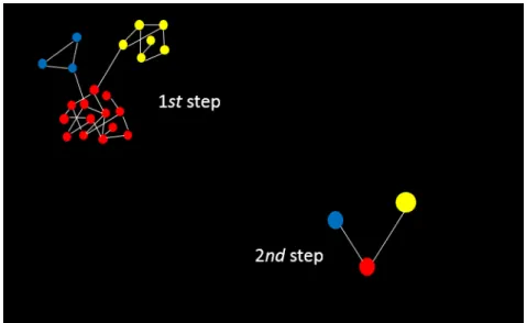
8 For a simple example: the subgraphs and the auxiliary graph determined, respectively, in the first phase and in the second phase of the proposed hierarchical consensus method. . . 70 9 Examples of subgraphs generation where one node is shared
between two subgraphs. . . 74 10 Adjacency matrices of a random geometric graph. On the
left an example with100nodes, on the right an example of graph with300nodes. . . 84 11 Number of steps to reach the consensus state with a
ran-dom geometric graph with100nodes. On the left: spectral clustering is used during the 1st phase of the algorithm; on the right: the1stphase of the algorithm is computed by applying thenearest supernode approachselecting the su-pernodeswith the4different types of seeds. . . 86
12 Number of steps to reach the consensus state with a ran-dom geometric graph with300nodes. On the left: spectral clustering is used during the 1st phase of the algorithm; on the right: the1stphase of the algorithm is computed by applying thenearest supernodeapproachselecting the su-pernodeswith the4different types of seeds. . . 87 13 Adjacency matrices of a planted partition graph with100
nodes. On the left an example withpin = 0.1andpout =
0.02, on the right an example withpin= 0.2andpout = 0.01. 89 14 Number of steps to reach the consensus state with a planted
partition graph with100nodes withpin= 0.1andpout =
0.02. On the left: spectral clustering for the1st phase of the algorithm; on the right:nearest supernode approach. . . . 90 15 Number of steps to reach the consensus state with a planted
partition graph with100nodes withpin= 0.2andpout =
0.01. On the left: spectral clustering for the1st phase of the algorithm; on the right: nearest supernode approachfor the1stphase. . . 91 16 Adjacency matrix of a planted partition graph with 300
nodes,pin= 0.2andpout = 0.01. . . 92 17 Number of steps to reach the consensus state with a planted
partition graph with300nodes withpin= 0.2andpout =
0.01. On the left: spectral clustering for the1st phase of the algorithm; on the right: nearest supernode approachfor the1stphase. . . 93 18 Adjacency matrices of a PA model. On the left an example
with100nodes, on the right an example with300nodes. . 93 19 Number of steps to reach the consensus state with a PA
model with100nodes. On the left: spectral clustering for the1stphase of the algorithm; on the right:nearest supern-ode approachfor the1stphase of the method. . . 94
20 Number of steps to reach the consensus state with a PA model with300nodes. On the left: spectral clustering for the1stphase of the algorithm; on the right:nearest supern-ode approachfor the1stphase of the method. . . 95 21 A nearly complete graph with a node attached to only one
node of the complete part. . . 96 22 Choice of the subset S to determine an upper bound on
the Cheeger’s constant for the basisantenna effectmodel. . 98 23 A complete graph on the left and a sparser one, on the
right, with a node attached to only one node of the original graph. . . 99 24 Second–largest eigenvalue modulus when a complete graph
with theantenna effectis considered. . . 100 25 Second–largest eigenvalue modulus when a sparser graph
than the complete one presents theantenna effect. . . 101 26 Adjacency matrix of a planted partition graph with 100
nodes,pin= 0.2andpout = 0.01. . . 102 27 Subgraphs determined by the hierarchical method with
clustering coefficient as seed. In the adjacency matrix on the right is shown theantenna effect. . . 103 28 Planted partition graph with 100 nodes, pin = 0.1 and
pout = 0.02. In blue: number of steps required by the original hierarchical method; in red: number of steps re-assigning the nodes with degree1to other subgraphs. . . . 105 29 Planted partition graph with 300 nodes, pin = 0.2 and
pout = 0.01. In blue: number of steps required by the original hierarchical method; in red: number of steps re-assigning the nodes with degree1to other subgraphs. . . . 106 30 Subgraphs determined by the hierarchical method when
31 Example of a discrete approximation of the manifold the data lie one. The red points denote negative samples, the blue ones belong to the positive class, while the black points represent unlabeled samples. . . 115 32 Ground truth. . . 131 33 Output of the SVM classifier(l= 200)on the left. Output
of the Laplacian SVM on the right. . . 132 34 ROC curves of the three classifiers computed by changing
the percentage of the positive samples over the total num-ber of samples. . . 133 35 Examples of imaging and spectroscopic quantitative
pa-rameters used as features for SVM analysis: manual mor-phometry (A); DTI FA and MD quantification by ROIs (B) and histograms (C) analysis; semi–automatic segmenta-tion of deep brain structures (D); cerebellar volume of in-terest localization (E) and corresponding1H–MR
metabo-lites spectrum (F). . . 143 36 Adjacency matrix when the entire dataset is considered,
fixing the number of nearest neighborsk= 40. . . 152 37 Comparison between the ROC curves obtained when the
entire set of features is considered (blue curve) and when only a subset with the first20ranked features is used (green curve). On the left the results without using graph–based features, on the right the curves obtained when graph– based features are added to the dataset. . . 153 38 Frequency of the first40ranked features in the13binary
classification problems “one disorder vs another” and “one disorder vs all”. . . 154 39 Chain graph with6nodes. . . 175 40 Two complete graphs connected by an edge. . . 176 41 All the possible cuts that divide two complete graphs
List of Tables
1 “0vs1h” binary classification problem, when the setsS1
andS2are obtained by a random partitioning of the dataset.128
2 “0vs1h” binary classification problem, when the setsS1
and S2 are defined, respectively, as the subset of objects
with latitude greater than or equal to 2750(expressed in pixel units), and the subset of objects with latitude smaller than the same threshold. . . 128
3 “0vs1h” binary classification problem, when the setsS1
and S2 are defined, respectively, as the subset of objects
with longitude smaller than or equal to 2400(expressed in pixel units), and the subset of objects with longitude greater than the same threshold. . . 129
4 “0 vs1” binary classification problem, when the sets S1
5 “0 vs1” binary classification problem, when the sets S1
and S2 are defined, respectively, as the subset of objects
with latitude greater than or equal to 2750(expressed in pixel units), and the subset of objects with latitude smaller than the same threshold. . . 130
6 “0 vs1” binary classification problem, when the sets S1
and S2 are defined, respectively, as the subset of objects
with longitude smaller than or equal to 2400(expressed in pixel units), and the subset of objects with longitude greater than the same threshold. . . 130
7 Demographic and clinical features of the study sample. . . 142 8 Accuracy in the binary classification problem “PD vs
an-other” varying the dimension of the set of features consid-ered. . . 155
9 Accuracy, sensitivity and specificity of SVMs in binary clas-sification problems “one disorder vs all”. Left column: results obtained without graph-based features; right col-umn: results obtained by using graphs to extract more fea-tures to provide to the classifiers. The stars specify when a statistically significant improvement is obtained when us-ing graph–based features. . . 156
10 Mean and standard deviation over the entire set of values of the regularization parameterCof the accuracies of the binary problems “one disorder vs all”. Graph–based fea-tures are not considered. . . 156
11 Mean and standard deviation over the entire set of values of the regularization parameterCof the accuracies of the binary problems “one disorder vs all”. Graph–based fea-tures are added to the original dataset. . . 156
12 Accuracy, sensitivity and specificity of SVMs in binary clas-sification problems “one disorder vs another”. Left col-umn: results obtained without graph-based features; right column: results obtained by using graphs to extract more features to provide to the classifiers. The stars specify when a statistically significant improvement is obtained when using graph–based features. . . 157 13 Mean and standard deviation over the entire set of values
of the regularization parameterCof the accuracies of the binary problems “one disorder vs another”. Graph–based features are not considered. . . 157 14 Mean and standard deviation over the entire set of values
of the regularization parameterCof the accuracies of the binary problems “one disorder vs another”. Graph–based features are added to the original dataset. . . 158 15 Optimal number ofknearest neighbors and features, with
the corresponding best accuracy, for the binary problems “one disorder vs another”. . . 158 16 Optimal number ofknearest neighbors and features, with
the corresponding best accuracy, for the binary problems “one disorder vs all”. . . 159 17 Optimal number ofknearest neighbors and features, with
the corresponding best accuracy, for the two multi–class classification problems. . . 159 18 Confusion matrices: on the left the 4–class classification
problem, on the right the 3–class classification problem. Graphs are not used to extract additional features. . . 160 19 Confusion matrices: on the left 4–class classification
prob-lem, on the right the 3–class classification problem. Graph– based features are added. . . 160
Vita
February 5, 1987 Born, San Giovanni in Persiceto (BO), Italy
2006–2009 B.SC in Matematics Mark: 110/110 cum laude University of Bologna Bologna, Italy
2009–2011 M.SC in Matematics
Mark: 110/110 cum laude University of Bologna Bologna, Italy
2013–present PhD candidate
IMT School for Advanced Studies Lucca, Italy
Publications
Papers in international journals
• G. Gnecco, R. Morisi, G. Roth, M. Sanguineti, A. C. Taramasso, “Su-pervised and semi–su“Su-pervised classifiers for the detection of flood– prone areas”, Soft Computing, pp. 1–13, 2015
• G. Gnecco, R. Morisi, A. Bemporad, “Sparse solutions to the av-erage consensus problem via various regularization of the fastest mixing Markov–chain problem”, IEEE Transactions on Network Science and Engineering, vol. 2, n. 3, pp. 97–111, 2015
• R. Morisi, B. Donini, N. Lanconelli, J. Rosengarden, J. Morgan, S. Harden, N. Curzen, “Semi–automated Scar Detection in Delayed Enhanced Cardiac Magnetic Resonance Images”, International Jour-nal of Modern Physics C (IJMPC), vol. 26, n.1, 2015
• C. Rusu, R. Morisi, D. Boschetto, R. Dharmakumar, S. A. Tsaftaris, “Synthetic Generation of Myocardial Blood–Oxygen–Level–dependent MRI Time Series Via Structural Sparse Decomposition Modeling”, IEEE Transactions on Medical Imaging, vol. 33, n. 7, pp. 1422–1433, 2014
• R. Morisi, G. Gnecco, N. Lanconelli, S. Zanigni, D. Manners, C. Testa, S. Evangelisti, L. L. Gramegna, C. Bianchini, P. Cortelli, C. Tonon, R. Lodi, “Binary and multi–class classification of parkinso-nian disorders with support vector machines based on quantitative brain MR and graph–based features”, Movement Disorders (sub-mitted)
• Rita Morisi, Giorgio Gnecco, Alberto Bemporad “A hierarchical consensus method for the approximation of the consensus state, based on clustering and spectral graph theory”, Engineering Ap-plications of Artificial Intelligence (submitted)
Conference papers
• L. L. Gramegna, C. Testa, R. Morisi, S. Zanigni, G. Gnecco, N. Lan-conelli, D. N. Manners, S. Evangelisti, P. Cortelli, C. Tonon, R. Lodi, “Binary and multi–class classification of parkinsonian disorders with support vector machines based on quantitative brain MR and graph– based features”, ISMRM Italian Chapter, 2016
• G. Gnecco, A. Bemporad, R. Morisi, M. Gori, M. Sanguineti, “On-line learning as an LQG optimal control problem with random ma-trices”, Proceedings of IEEE ECC 2015
• R. Morisi, G. Gnecco, N. Lanconelli, et al., “Binary and multi–class Parkinsonian disorders classification using Support Vector Machines”, In: Lecture Notes in Computer Science, Springer, 2015
• G. Gnecco, R. Morisi, and A. Bemporad, “Sparse Solutions to the Average Consensus Problem vial1–norm Regularization of the Fastest
Mixing Markov–Chain Problem”, In: Proceedings of the 53rd An-nual Conference on Decision and Control (CDC), IEEE, pp. 2228-2233., ISBN 978-1-4799-7746-8, 2014
• L. Lara-Rodriguez, S. Vera, F. Perez, N. Lanconelli, R. Morisi, B.Donini, et al., “Supervised Learning Modelization and Segmentation of Car-diac Scar in Delayed Enhanced MRI”. Lecture Notes in Computer Science, vol. 7746, 2013, Statistical Atlases and Computational Mod-els of the Heart, Imaging and Modelling Challenges
• L. Lara-Rodriguez, S. Vera, F. Perez, N. Lanconelli, R. Morisi, et al., “Cardiac scar detection, segmentation and quantification in MRI images for ICD treatment planning”, International Journal of Com-puter Assisted Radiology and Surgery, vol. 7, s. 1 (Proceedings of CARS 2012, Pisa, Italy), 2012.
• R. Morisi, R. Dharmakumar, and S. A. Tsaftaris, “Unsupervised Is-chemia Detection at Rest with CP–BOLD Cardiac MRI: A Simu-lation Study Employing Independent Component Analysis”, Pre-sented for the International Society of Magnetic Resonance in Medicine (ISMRM) Meeting, Milan, May 2014, Magna Cum Laude Award re-ceived
Abstract
Graphs are powerful data structure for representing objects and their relationships. They are extremely useful in the study of dynamical systems, evaluating how different agents in-teract among each other and behave. An example is repre-sented by the consensus problem where a graph models a set of agents that locally interact and exchange their opin-ions with the aim of reaching a common opinion (consen-sus state). At the same time, many learning techniques rely on graphs exploiting their potentialities in modeling the rela-tionships between data and determining additional features related to the data similarities. To study both the consensus problem and specific machine learning applications based on graphs, the study of the spectral properties of graphs reveals fundamental. In the consensus problem, the convergence rate to the consensus state strictly depends on the spectral pro-perties of the transition probability matrix associated to the agents network. Whereas graphs and their spectral proper-ties are fundamental in determining learning algorithms able to capture the structure of a dataset. We propose a theoretical and numerical study of the spectral properties of a network of agents that interact with the aim of increasing the rate of convergence to the consensus state keeping as sparse as pos-sible the graph involved. Experimental results demonstrate the capability of the proposed approach in reaching the con-sensus state faster than a classical approach. We then inve-stigate the potentialities of graphs when applied in classifica-tion problems. The results achieved highlight the importance of graphs and their spectral properties handling with both semi–supervised and supervised learning problems.
Part I
Introduction and
background
1
Introduction
1.1
Graphs versatility and applications
Graphs are a general and powerful data structure for objects repsentation; they are used to model entities, their attributes and their re-lationships (1). Generally speaking, a graph is characterized by a set of nodes, which represent the different entities, and a set of edges that link pairs of nodes and represent the interconnections between the nodes. In particular, a graph is directed if the edges have a direction associated with them, undirected otherwise. Nowadays, graphs are becoming in-creasingly important in modeling structures and their interactions, with broad applications including computer vision, bioinformatics, text re-trieval, and Web analysis, where they represent a useful tool for sear-ching and for community discovery (2). In modeling physical and bio-logical processes (3; 4; 5) graphs, for instance, are used to represent con-nections between interacting parts of a system, to model the dynamics of a physical process, disease propagation, as well as the evolution of po-pulations in an ecosystem (6). Several biological systems, in fact, can be usefully represented as networks. Examples are the genetic regulatory network and the food web network, which can be modeled by a graph with nodes representing species in an ecosystem and directed edges
in-dicating which species prey on the other (3). In addition, they are widely used in the study of social systems (7), where a social network is a set of people or groups of people with some patterns of contacts or interactions between them (8). The patterns of friendships between individuals, busi-ness relationships between companies are examples of social networks (3). At the same time, graphs represent a useful tool to study the flow of information between different systems (9), how news and information spread between single individuals and groups of agents (10; 11), and to analyze the flow of traffic on roads (10). Finally, another application of graphs is represented by the network of citations between academic pa-pers. In this case, the nodes of the network are the articles, while the directed edges indicate which articles cite the others.
At the same time, in the machine learning field different methods rely on graphs. There are both unsupervised and supervised learning techniques that make use of graphs. Regarding unsupervised and semi– supervised methods, graphs can provide a model of the manifold where the data lie on and they are also used to determine clusters of similar data (12). In a supervised context, graphs can be exploited to infer la-bels or numerical values attached to nodes, to extract novel and useful knowledge from data, and additional features (13). In addition, they can be also combined with other learning techniques, such as the so–called kernel methods (14), providing a useful tool to deal with several learning problems.
Moreover, in (15) the idea of constructing kernels on the nodes of graphs was first proposed, with the aim of capturing the relationships between data points induced by the local structure of the graph; the work (16), instead, focuses on kernels capturing the similarity of whole graphs (that idea was first proposed by (17)). For both these types of graph ker-nels, the challenge is to define a kernel that captures the semantics inher-ent in the graph structure (16). Examples of application of graph kernels can be found, for instance, in (18), where they are used to compare bio-logical networks, or in (19), for the prediction of protein function.
Finally, another application of graphs in the field of patter recogni-tion and computer vision is represented by the graph matching problem
(20; 21). This problem consists in searching for an edge–preserving map-ping between the nodes of two graphs (22). Specifically, in the field of computer vision, many problems are formulated as an attributed graph matching problem; the nodes of the graphs correspond to local features of the image and edges correspond to relational aspects between fea-tures. The final goal is to find a correspondence between nodes of the two graphs such that they “look similar” (23). In a pattern recognition context, instead, the graph matching problem can be found, for instance, in the human faces recognition problem (24).
Beside the problems already introduced, additional learning problems that rely on graphs concern, for instance, the problems of character recog-nition, shape analysis (25), Web document analysis (26; 27; 28) and data mining (29).
1.2
Problem statement
One of the problems investigated in the theory of dynamical systems is the consensus problem. This kind of situation is characterized by a group of agents that locally interact and exchange opinions. They are modeled by a graph with nodes corresponding to the agents and edges representing their interconnections. For instance, if the graph of inter-connections is undirected, an edge between two different agents (i.e., nodes) represents the possibility for one of the two to receive informa-tion from the other and vice–versa (30; 31). Agents influence each other depending on the strength of the interconnections between them (32). In particular, a “consensus algorithm” is an interaction rule that specifies the information exchange between an agent and all of its neighbors on the network (33). The final goal of this problem is to have all the agents agree upon a common opinion, a “consensus”, that means to reach an agreement regarding a certain quantity of interest that depends on the state of all agents. Several applications of this kind of problem exist. For instance, the consensus problem arises when dealing with the collective behavior of networked agents (34), in the context of multiagent coordi-nation (35; 36), sensor networks (37) and many other applications (38).
At the same time different consensus algorithms and studies have been developed (39; 40; 41).
In this dissertation we focus on the average consensus problem, where the graph of interconnections is undirected (i.e., the edges are not orien-tated, thus an agent connected to another can communicate with him and vice–versa), and the final consensus state is given by the average of their initial opinions (42). In particular we are interested in studying the convergence rate to the consensus state. In this context, the spectral properties of the network which models the group of agents play a cru-cial role. In particular, the Laplacian matrix and its spectral properties (43; 44) are fundamental to study how the network of agents evolves. Studies related to the convergence rate to the consensus state have been developed, for instance, in (45; 46; 47), while in (48) it is studied the re-lated problem of the mixing time.
We intend to focus from both a theoretical and practical point of view on the spectral properties of the network involved in order to increase the convergence rate to the consensus state keeping, at the same time, as sparse as possible the agents network. We require, in fact, to obtain solutions able to keep the cost of communications between the different agents small.
On the other hand, in the thesis the spectral properties of graphs are also exploited in a machine learning context. Beside the application of graphs to the study of dynamical systems and of interconnections of indi-viduals, we intend to study the potentiality of graphs in their application to classification problems. In particular, we aim at analyzing the spectral properties of graphs, previously evaluated in the consensus problem, in a semi–supervised learning context. We focus on the application of a semi– supervised learning technique that relies on a graph built on the dataset for the classification of flood–prone areas. Graphs, in situations where both labeled and unlabeled data are present, represent a fundamental tool to handle with both such types of data, making possible to extract additional information from the unlabeled data. The spectral properties of graphs, in this context, reveal to be fundamental to estimate the data probability distribution. This knowledge is fundamental to compute a
classifier able to usually achieve better performance than a classical one that does not rely on the spectral properties of a graph adequately com-puted on the dataset.
Finally, the potentialities of graphs in a learning context are shown in another classification problem. We study and apply graphs in a classifi-cation problem of parkinsonian disorders in order to model the dataset, extracting additional graph–based features from the data. We aim at computing features that capture the similarities between data belonging to the same class and the dissimilarities between data coming from dif-ferent classes. The comparison between this approach and a classical one that does not rely on graphs highlights again the capabilities of graphs in modeling data and extracting additional and useful information.
1.3
Challenges and scientific contributions
The main contribution of this dissertation relies on the theoretical and practical studies of graphs and their spectral properties in both the con-trol field and in machine learning problems. In Part II we present orig-inal theoretical studies related to the solution of the consensus problem and we provide theoretical and practical solutions able to sparsify the network of the agents, keeping at the same time the rate of convergence to the consensus state sufficiently high. We then focus on a novel ap-proach able to increase the convergence rate to the consensus state di-viding the original network in several subgraphs. Again, we ground our study on graph spectral theory and in particular on the application of the Cheeger’s inequality (49).Beside our investigation of the consensus problem, in Part III, we also provide novel contributions in specific classification problems. We high-light the potentiality of a semi–supervised learning technique based on graphs in improving the classification performance of a classical super-vised classifier that does not exploit spectral properties of graphs. Fi-nally, we conclude our study on graphs evaluating their capabilities in modeling a dataset and extracting additional information from it.
2 we report and describe fundamental graph features that are consid-ered in the following chapters. In particular we briefly introduce spectral graph theory and its notions. The study of the eigenvalues and eigenvec-tors of the matrices related to graphs represents the common denomina-tor between the two different topics treated in this dissertation.
InChapter 3the consensus problem is presented. We introduce the problem of dealing with a large number of agents that locally interact and have to reach a common opinion as fast as possible. We focus on the study of the graph topology determining the structure of the net-work that leads to the fastest convergence rate to the consensus state. In particular, we are interested in determining a sparse variation of the problem, with the aim of determining a sparse graph with a fast conver-gence rate to the consensus state. Dealing with large networks is, from a computational point of view, expensive and time consuming especially when huge networks are considered. Hence, determining a method able to provide satisfactory results in terms of convergence rate to the consen-sus state maintaining, at the same time, the graph as sparse as possible is useful and advantageous in many applications where large networks are considered. InChapter 4we continue the study on the consensus prob-lem and the rate of convergence to the consensus state. Differently from the previous chapter, where a convex optimization problem is consid-ered, now the idea is to opportunely divide the original network in dif-ferent subnetworks (i.e., subsets of agents), having fast convergence rate to their local consensus state. We thus decompose the consensus prob-lem in many consensus subprobprob-lems and then we investigate the final consensus problem “merging” the local consensus states previously com-puted. A suitable technique able to extract from the original graph differ-ent subgraphs where the convergence rate to their own consensus state is fast, reveals useful to increase the convergence rate to the consensus state computed on the original network, without using such technique. InChapter 5the spectral properties of graphs are again studied but they are applied in a different context. A machine learning problem is con-sidered, dealing with a semi–supervised classification problem, where both labeled and unlabeled data are provided to a classifier. In
particu-lar, we apply a semi–supervised learning technique for the classification of flood–prone areas. The main purpose of the specific study is the eval-uation of the capabilities of a semi–supervised learning technique that exploits the spectral properties of a graph used to model the manifold where the data lie on. We compare the results achieved by the semi– supervised classifier with the ones achieved by a supervised learning technique trained on the labeled data only. A graph–based learning tech-nique reveals suitable for this particular classification context. Finally, in
Chapter 6we show an additional application of graphs in the machine learning field. Again a classification problem is presented, dealing with different parkinsonian disorders. Contrary to the previous problem, in this case graphs are not used in the learning algorithm, but they provide a model of the dataset highlighting the similarities and dissimilarities be-tween the data. A graph is built on the dataset with the aim of extracting additional features from the data that have to be classified. We observe that graphs are a powerful structure able to provide useful information to improve the classification results achieved when graph–based features are not added to the dataset. Finally,Chapter 7offers a final discussion and the concluding remarks highlighting the important developments achieved in this work and future improvements to carry out.
2
Introduction to graphs and spectral
properties
2.1
Introduction
In this preliminary chapter we provide a brief introduction to graphs. We introduce the basic notations and information necessary to deal with the arguments described later. We first recall the generic notations used to introduce and describe graphs, then a selection of features related to both single nodes and subsets of nodes in a graph will be provided. We introduce only the notations that will be recalled and used in the fol-lowing chapters. Subsequently, we will focus on spectral graph theory whose properties will be discussed in Chapters 3 and 4, where the con-sensus problem is studied, and Chapter 5 where semi–supervised learn-ing techniques are studied and applied. In particular, we will focus on the study of the eigenvalues of the Laplacian matrix of a graph introduc-ing important results that will be used and considered in the study of the consensus problem.
2.2
Graph representation
A graphGconsists of a finite set of nodes (or equivalently vertexes)
V and a set of edgesE; its representation is given by a pairG= (V, E). From now on, we will indicate withvia generic node in the vertex set
V, while witheij∈Ewe indicate the edge between a couple of nodesvi andvj. |V|indicates the cardinality ofV; thus, ifV = {v1, v2, . . . , vN}, it follows that|V| = N. We are interested in undirected graphs where no orientation in the edges is present, while weighted and unweighted graphs will be both taken in consideration. The difference between the two is related to the presence or not of a weight associated to the edges between the different pairs of nodes. We will use the same notation to indicate both the unweighted and weighted graphs. For the latter we will sometimes indicate withWthe weighted adjacency matrix (used ex-tensively in the following chapters) whose entrieswijspecify the weight associated to each edgeeij. The weightwijis a real non negative number that represents the strength of the connection between the pair of nodes
viandvj,∀i, j= 1, . . . , N. Note that, for undirected graphs,wij=wji. As just introduced for weighted graphs, we recall that both a weighted and an unweighted graph can be entirely represented by a matrix A
which is called the adjacency matrix. If|V|=N, the adjacency matrixA
is anN×Nmatrix whose entries are defined as
aij=
(
wij if (vi, vj)are connected by an edge
0 otherwise
in the case of weighted graphs. Sometimes we will use eitherAorW to indicate the adjacency matrix in the weighted case. If unweighted graphs are considered, the adjacency matrix is a binary matrixAwith entries:
aij=
(
1 if (vi, vj)are connected by an edge
0 otherwise
Again, if the graph is undirected, the adjacency matrixAis symmetric. Note that, in this introductory chapter, when defining graph features and important quantities related to graphs, we do not consider nodes
with self–loops. Anyway, in Chapters 3 and 4 where the consensus prob-lem is studied, we will introduce graphs presenting self–loops.
In the following section we first provide a description of a series of graph features (50; 51; 52; 53) that will be used in the following chapters.
2.2.1
Graphs features and fundamental notions
Nodes definitions and features
LetGbe a generic graph, withNnodes, i.e.,|V|=N;Gcould be either a weighted graph or an unweighted one. We now report some measures of the importance of a generic nodevi ∈ G; indices that define the im-portance of a node are the so–called centrality measures (6; 54). First, we mention the degree of a nodevi, withi = 1, . . . , N, which is defined as
di = P N
j=iaij. It is the sum of the edge values incident to the vertex, where each of these edges has value1 in the unweighted case,wij oth-erwise. The sum of the degrees of all the vertices is the total degree of a graph. The degree matrixDof a graph, instead, is defined as the diago-nal matrix with the degreesd1, . . . , dN on the main diagonal. In general an important node is involved in a large number of interactions.
Beside the degree of a node, before introducing other centrality mea-sures, we need to introduce the natural distance metric between pairs of nodes; this measure is the length of the shortest path between two nodes. More precisely, given two nodesviandvj, a shortest path between them is defined as any of the paths (i.e., a sequence of edges which connect the two nodes) with the minimum number of edges (in the unweighted case) or with the minimum sum of the weights of its constituent edges, for weighted graphs. Thus, as previously mentioned, the distance be-tween pairs of nodes is measured as the length of any of the shortest paths between them, i.e., the sum of the weights of the edges in such shortest path. We define the length of the shortest path between nodesvi andvjasδ(vi, vj).
• closeness centrality: given a nodevi, it is defined as Cc(vi) := 1 P vjδ(vi, vj) .
This feature defines the importance of a node measuring if this node is “close” to and can communicate quickly with the other nodes in the graph;
• betweennes centrality: given a nodeviinG, this centrality measure is defined in the following way:
Bc(vi) := X vj6=vi6=vk∈V σvj,vk(vi) σvj,vk ,
whereσvj,vkis the total number of shortest paths from nodevjand
node vk, while σvj,vk(vi) is the number of those paths that pass
throughvi. This measure tells us that an important node lies on a high proportion of shortest paths between other nodes.
We then mention the vertex eccentricitye(vi)of a generic node vi de-fined ase(vi) = max{δ(vi, vj) : vj ∈ V}; the radius r(G)of a graph that isr(G) = min{e(vi) :vi ∈ V}. Finally, we introduce the clustering coefficient of a nodevi that is a measure of the degree to which nodes in a graph tend to cluster together. More precisely, defining the neigh-borhoodNi of a vertexvias the set made of its immediately connected neighbors, i.e.,Ni = {vj : eij ∈ E}, the clustering coefficientC(vi)of nodeviis defined as:
C(vi) =
2|{ejk:vj, vk ∈Ni, ejk∈E}|
ki(ki−1)
,
wherekiis the number of neighbors of nodevi.
Subgraphs notions
From the vertex setV of a graph, it is possible to consider a generic subset of verticesS ⊆ V that define a subgraph of the original graphG. In
particular, given the subsetS ⊆V, we denote its complement asV \S
or, equivalently asS¯. The “size” of subsetSis defined either as |S|:=the number of vertices in S,
or as
vol(S) :=X
i∈S
di. (2.1)
In particular, we say that a subsetS is connected if any two vertices inScan be joined by a path such that all intermediate nodes also lie inS. Moreover, a subsetS is called a connected component if it is connected and if there are no connections between nodes inSandS¯. Finally, given two disjoint subsetsS, T ⊂V, we define thecutbetween them as:
cut(S, T) := X
i∈S,j∈T
wij (2.2)
Thus, thecutbetween the sets of nodesS andT is the sum of the edge values with an extremity inSand another inT. Finally, we introduce the definition of connected graph that will be extensively used in Chapters 3 and 4. An undirected graphGis connected if each pair of vertices forms the endpoints of a path (i.e., for eachviandvjnodes inGthere is a path which connects them). In addition, when dealing with directed graphs, a directed graphGis said to be strongly connected if for each two vertices there are paths from one to the other in both directions. The notations just introduced are necessary to deal with the consensus problem and the particular development described in Chapter 4.
Before diving into spectral graph theory and its properties, we de-scribe some methods used to build a graph that will be considered in Chapters 5 and 6.
2.2.2
Similarity graphs
Given a datasetX ={x1, . . . , xN}, wherexi ∈Rn, withi= 1, . . . , N, aren–dimensional vectors, if one is interested in building a graph G= (V, E)on these data points, either a weighted one or an unweighted one,
it is necessary to define a notion of similaritysij ≥0between all pairs of dataxiandxj. More precisely, each data pointxicorresponds to a node
vi, while the similarity measuresij encodes the strength of the connec-tion between pointsxiandxj. In general, these two points are connected by an edgeeij if the similarity measuressij is positive or larger than a certain threshold. We use the term similarity measure, or equivalently, distance measure to describe three techniques commonly used to define a graph starting from the points; they are:
• –neighborhood graph: the points connected are those with distances
sij, withi= 1, . . . , N, smaller than a given >0;
• k-nearest neighbor graph: for a givenk, a vertexvj, corresponding to an elementxj, is connected to another vertexviifvj is among the
knearest neighbors ofvi. Since we will deal with only undirected graphs, and the one built following this rule is a directed one, one of the following ways to make the graph undirected can be ap-plied. Eitherviis connected tovjifviis among thek–nearest neigh-bors ofvj orvice–versa, determining ak–nearest neighbor graph; or
vi and vj are connected by an edge ifvi is among the k–nearest neighbors ofvj andvj is among thek–nearest neighbors ofvi. The resulting graph is calledmutualk–nearest neighbor graph: this con-struction leads to a sparser graph than the previous one. Both un-weighted and un-weightedk-nearest neighbor graphs/mutualk–nearest neighbor graphscan be built depending on the choice of assigning the value1to the edges connecting the nodes or a weight related to the distance between the pairs of nodes;
• fully connected graph: between all the possible pairs of points the Gaussian similarity functionsij = exp(kxi−xjk
2
2σ2 )is computed
de-termining the weighted matrixW with entrieswij=sij.
From the similarity measures, depending on the particular applica-tion and purpose one is dealing with, either a weighted graph can be obtained by using as edge weights the similarity measures themselves or an unweighted graph can be built. It can be obtained by
threshold-ing the values of the weights and assignthreshold-ing an edge with value1only between pairs of pointsxiandxjwith similaritysijthat satisfies certain requirements. Otherwise, if ak–nearest neighbor graph is considered, it can be transformed into an unweighted one by assigning value1to the edges instead of their original weight (55).
We have introduced a brief overview on graph notations useful for the studies presented in the next chapters. We now continue the intro-duction to graphs focusing on spectral graph theory and its properties. Our main goal is to introduce definitions and techniques able to deter-mine clusters inside a graph. In Chapter 4, in fact, we will need to de-termine clusters inside a single graph in order to increase the rate of con-vergence to the consensus state.
2.3
Spectral graph theory
This branch of graph theory is concerned with the analysis of graphs by using algebraic properties of associated matrices. In particular, it studies the relation between graph properties and the spectrum of the adjacency matrix or the Laplacian matrix (56). The latter matrix is de-fined asL=D−A, whereDis the degree matrix of a graph, whileAis either the binary adjacency matrix in the case of unweighted graphs or the weighted adjacency matrix if weighted graphs are considered. More specifically,Lis the matrix with components equal to:
Lij = di if i = j
−1 ifviandvjare connected by an edge
0 otherwise
For our purposes we denote withξi, withi= 0, . . . , N−1the eigenval-ues of the Laplacian matrix, where, in the following, the eigenvaleigenval-ues are considered in a non–decreasing order, i.e.,ξ0≤ξ1, . . . ,≤ξN−1. Note that
L, defined as above, is also called unnormalized Laplacian matrix; in the following we list some properties ofLthat can be found, for instance in (55; 57; 58).
• ∀x∈RN one hasxTLx=1 2
PN
i,j=1wij(xi−xj) 2;
• Lis a symmetric positive-semi-definite matrix;
• the smallest eigenvalue ofLis ξ0 = 0. Moreover, the indicator vector 1= (1,· · · ,1)T is an eigenvector associated with the eigenvalue0; • from the second property it follows that the eigenvalues ofLare real and
non–negative values
0 =ξ0≤ξ1, . . . ,≤ξN−1.
Another important property ofLthat is fundamental in spectral graph theory is the following:
Remark 2. The multiplicity of the eigenvalue0ofLis equal to the number of connected components of the graph, and a basis of the associated eigenspace is made of the indicator vectors of such connected components.
We refer to (55) for the proof of the propositions stated above. In many applications two possible variations can be used instead of the unnormalized Laplacian matrixL. They are:
• the normalized Laplacian matrix given byLN =I−D−
1 2AD−12, • the random walk Laplacian matrix defined asLrw=I−D−1A. Where, again,Acan be either a binary or a weighted adjacency matrix. If graphs with isolated nodes are considered (i.e., a graphGwith at least a nodevi with degreedi = 0), we introduce the following notation re-ported in (59):
d−1ii =d−12
ii = 0∀visuch thatdi= 0 In particular, the structure of matrixLN is the following:
LN ij= 1 ifdi6= 0andi=j −√1 didj if
(vi, vj)are connected by an edge anddi6= 0
while Lrw ij= 1 ifdi6= 0andi=j −1
di if(vi, vj)are connected by an edge anddi6= 0
0 otherwise
.
Similar properties like the ones listed in Remarks 1 and 2 hold for the two versions of the normalized Laplacian matrices, that can be found, for instance, in (49; 60; 61; 62). In the following we will indicate withξi the eigenvalues of both the unnormalized and the normalized Laplacian matrix, depending on the application we will consider.
Now, our purpose is twofold. We first intend to introduce some fun-damental notions of spectral clustering, because, as we will describe in Chapter 4, we need a method able to determine clusters inside a graph in order to increase the convergence rate to the consensus state. Then, we aim at introducing some important quantities related to the set of eigen-values ofLin order to better understand the topology of a given graph (49). Of course, these two tasks are strongly related.
2.3.1
Spectral clustering technique
The goal of spectral clustering is to cluster data making use of the eigenvalues and eigenvectors of the Laplacian matrix. In particular, for spectral clustering algorithms, both the unnormalized version and the normalized version of the Laplacian matrix can be used. All the spec-tral clustering algorithms are able to cluster a set of data points X =
{x1, . . . , xN} by means of the eigenvectors of the Laplacian. More pre-cisely, as stated in Remark 2, by considering the multiplicity of the eigen-value0of the Laplacian matrix, it is possible to estimate the number of clusters inside a graph. In fact, as shown in (63), if a connected compo-nent has a structure withk “apparent” clusters, the firstkeigenvalues will be close to0, while starting from thek+ 1-th eigenvalue, their value will be significantly larger than0. In this case, the projection of the data pointsxion the subspace defined by the firstkeigenvectors correspond-ing to thek smallest eigenvaluesξj, with j = 0, . . . , k−1, makes the clustering process easier to be performed. In particular, without going
into details, a spectral clustering algorithm, starting from the similarity graphW and the numberkof clusters that are supposed to be present in the original graph, computes the firstkeigenvectorsu0, . . . , uk−1of the
unnormalized or normalized Laplacian matrix. It subsequently builds a matrixU ∈ RN×k containing the vectorsu0, . . . , uk−1as columns.
Fi-nally, the algorithm clusters the new points corresponding to the rows of
U(that are the original nodes projected in the newk–dimensional space spanned by the firstk eigenvectors of the Laplacian matrix), with the
k–means clustering algorithm (64).
The spectral clustering technique can be derived starting from differ-ent theories and points of view. In the following section we briefly list some of these theories and the connection with spectral clustering. For further information and for the proofs of the statements we will intro-duce, the reader is referred to (55; 65).
2.3.2
Spectral clustering points of view
LetX ={x1, . . . , xN}be a set of data points and letGthe correspond-ing similarity graphGwith adjacency matrixW built following one of the methods described in Section 2.2.2. Spectral clustering can be ex-plained by the following theories.
Graph cut point of view
As previously mentioned, clustering tends to separate points in dif-ferent groups according to their similarities; it means that the goal of this kind of method is to partition a graph such that the edges between differ-ent groups have a very low weight, while edges inside the same cluster have high weight. This problem can be translated in solving the mincut problem. More precisely, starting from the definition ofcutbetween two different subsets (Formula (2.2)), given a generic numberkof subsets, the mincut problem consists in determining the partitionS1, S2, . . . , Sk that minimizes
cut(S1, . . . , Sk) = k
X
i=1
cut(Si, Si). (2.3)
Thus, the minimization of (2.3) imposes the edges between different groups to have a very small weight. However, since the solution of problem (2.3) often leads to unsatisfactory results, in general, two different functions are preferred: RatioCut(S1, . . . , Sk) = k X i=1 cut(Si, Si) |Si| ; (2.4) Ncut(S1, . . . , Sk) = k X i=1 cut(Si, Si) vol(Si) . (2.5)
These two different functions are usually preferred since in many cases, the minimization of (2.3) determines a solution given by one in-dividual vertex separated from the rest of the graph. Thus, in order to have reasonably large clusters, minimizing either equation (2.4) or (2.5) which are normalized by the size of the subset, leads to a solution with reasonably large subsetsS1, S2, . . . , Sk. In particular, the RatioCut equa-tion measures the size of a subsetSiby its number of vertices|Si|, while the Ncut equation divides thecutby the weight vol(Si)of the edges in subsetSi. Now, it is possible to prove that spectral clustering represents a way to solve a relaxed versions of the RatioCut problem (Formula (2.4)) and the Normalized cut problem (Formula (2.5)) (55; 60; 61; 66).
Random walks point of view
Random walks on the similarity graph can be used to derive another possible explanation of spectral clustering. In particular, spectral cluster-ing can be associated to the problem of findcluster-ing a partition of the graph such that the random walk stays long within the same cluster and sel-dom jumps between clusters.
Defining bypijthe transition probability of jumping in one step from vertexvi to vertexvj, it is common to assume thatpij is proportional
to the edge weightwij; in particular, a possible choice ispij := wdij
i . It
follows that the transition matrixP= (pij)i,j=1,...,N of the random walks is defined by
P=D−1W,
that is strictly related to the normalized Laplacian, sinceLrw=I−P. In particular, this equivalence will be discussed in details in Chapter 3 and 4.
Now, as (67) shows there is a formal equivalence between the Ncut and the transition probabilities of random walks; thus, solving the Ncut minimization problem allows to determine a cut through the graph such that a random walk seldom passes through a cluster and another. This explains another spectral clustering point of view.
Matrix perturbation point of view
The last interpretation of spectral clustering derives from perturba-tion theory (68; 69). This studies how eigenvalues and eigenvectors of a matrix change if a small perturbation is added to the matrix itself. In particular, the formal basis for the perturbation approach to spectral clus-tering is the Davis–Kahan theorem (70).
Now, if we consider a disconnected graph withkconnected compo-nents, we know that the firstkeigenvectors ofLorLrware the indicator vectors of the clusters. If we then slightly perturb (i.e., by adding a small number of edges between nodes in different clusters) the original graph, the corresponding perturbed (normalized or unnormalized) Laplacian is a small perturbation of the original Laplacian matrix. Now, from Davis– Kahan theorem it follows that the relationship between matrix perturba-tion theory and spectral clustering resides on the choice of an appropri-ate intervalI that contains both the firstkeigenvalues of the Laplacian in the ideal case (disconnected graph withkconnected components) and the ones of the perturbed Laplacian matrix. In particular, the choice of the appropriate intervalIis easier the smaller the perturbation ofLand the larger the eigengap|ξk+1−ξk|. Finally, from Davis–Kahan theorem it follows that the larger the eigengap, the closer the eigenvectors of the
ideal case and the perturbed case, and hence the better spectral clustering works. For further details we refer to (55; 70).
In the next section a detailed study on the second smallest eigenvalue
ξ1of the normalized Laplacian matrixLNis carried out. This eigenvalue, in fact, is an indicator of the rate of convergence to the consensus state, argument that will be studied in the following two chapters.
2.3.3
Laplacian eigenvalues and their properties
In this section, we focus on the study of the Cheeger’s inequality, (see, e.g., (71)) which provides an upper and lower bound for the sec-ond smallest eigenvalueξ1of the normalized Laplacian matrixLN.
The Cheeger’s inequality, as described in (71) relates the eigenval-ues of the normalized Laplacian matrix associated to a graph with the Cheeger’s constant of the graph. In particular, ifG= (V, E)is a graph andS⊂V, denoting with∂(S)the boundary ofS, i.e.,
∂(S) :={(u, v)∈E:u∈S, v /∈S} the Cheeger’s constant is defined in the following way:
Φ(G) := min
S⊂V
|∂(S)|
min{vol(S),vol(V −S)}, (2.6) wherevol(S)is the volume of the subsetS ⊂V defined in Formula (2.1). Now, the relation between the Cheeger’s constant and the second smallest eigenvalueξ1of the normalized Laplacian matrix follows from
the Cheeger’s inequality:
Φ(G)2
2 ≤ξ1≤2Φ(G). (2.7)
The proof of Formula (2.7) can be found, for instance, in (71). It is proved for unweighted graphs without self-loops but the proof can be general-ized to weighted graphs with self-loops (see Section 5 in (71)).
A related results to the Cheeger’s inequality, is represented by he fol-lowing formula, that is again shown in (49) :
ξ1≥
1
whereD(G)is the diameter ofG, i.e., the maximum value of the shortest paths between any pair of nodes. From Formula (2.8), we can infer that
vol (G)being the same, ξ1 is larger when G is a “cluster” of vertices.
For instance, if we consider two subgraphs with the same volume, the smallerD(G)(i.e., the more a subgraph is “dense” or a cluster), the larger the lower bound onξ1; it is then expected thatξ1is larger. We will see in
Chapter 4 that Formulas (2.7) and (2.8) are useful to determine an upper and lower bound for the second smallest eigenvalue of the normalized Laplacian matrixξ1that is needed to estimate the rate of convergence to
the consensus state. In particular, we will see that, in order to achieve a fast convergence to the consensus state, one should avoid a situation where a graph, or a subgraph is made of two clusters “poorly” connected by a small number of edges, since in this case, the upper bound onξ1and
thus the value ofξ1is expected to be small.
2.4
Summary
In this chapter we provided a brief background on graph theory. The basic definitions and notions were introduced focusing on the descrip-tion of some features related to both single nodes and set of nodes that constitute subgraphs. The basic notations of spectral graph theory and its related quantities and properties were introduced too.
In the next chapter we will focus on the use of graphs in the study of dynamical systems. Our attention is channeled on the consensus prob-lem discussed first in Chapter 3 and then evaluated from a different point of view in Chapter 4. In particular, to deal with this kind of problem, the spectral properties of graphs will be evaluated and studied in details.
Subsequently in Chapters 5 and 6 graphs will be exploited in a ma-chine learning context. Again, the spectral properties of graphs will be considered to introduce an application in a classification problem of a semi–supervised learning technique, while graph–based features will be evaluated in another classification problem in order to extract additional and useful information from a dataset.
Part II
The consensus problem and
its graph of
3
The consensus problem and its sparse
variations
3.1
Introduction
The theory of complex systems deals with the study of the behavior of different types of systems made of agents that interact among each other; the study, for instance, of physical systems with particles that interact, social and economic networks, natural and ecological systems are typical examples (72). All of these situations are characterized by a large number of agents which interact among each other, without having, in general, a global knowledge about the structure of the system but interacting only locally with their neighbors (73; 74).
One particular study characterized by a network of agents that locally This chapter is partly based on:
• G. Gnecco, R. Morisi, A. Bemporad, “Sparse solutions to the average consensus problem via various regularizations of the fastest mixing Markov-chain problem”, IEEE Transactions on Network Science and Engineering, 2:97-111,2015
• G. Gnecco, R. Morisi, A. Bemporad, “Sparse solutions to the average consensus problem vial1–norm regularization of the fastest mixing Markov-chain problem”,
Proceedings of the IEEE International Conference on Decision and Control (CDC), 2014:2228-2233
interact among each other is the so–called consensus problem (30; 75). It consists in investigating how complex systems, constituted by the inter-connection of many units, behave with respect to the possibility of reach-ing consensus. The behavior of these systems is related on the dynamics of their units and on the topology of the connections between them. In particular, we are interested in studying the conditions under which a complex system has all its agents agree with the same opinion (the con-sensus state) and the time of convergence to that concon-sensus. In this work we focus on the study of the rate of convergence to the consensus state paying particular attention to the the structure of the graph of intercon-nections with the aim of keeping it as sparse as possible. In fact, when dealing with large graphs with high cost of communication between the different nodes, it reveals extremely useful to find a solution able to guar-antee the convergence to the consensus state as fast as possible reducing the number of interconnections, thus the communication costs, between the different agents. Starting from the formulation given in (48), the main contribution of the present work resides in the study from both a theo-retical and practical point of view of sparse solutions of the consensus problem with satisfactory rate of convergence to the consensus state.
We first provide an introduction to the model of the problem, see e.g., Section 3.2; then, in Section 3.3 we introduce the Fastest Mixing Markov–Chain (FMMC) Problem, which is concerned with the study of the topology of the network with the aim of determining the fastest mix-ing Markov chain on the graph (48). We then provide an additional theo-retical study and some variations of the FMMC Problem (see e.g., Section 3.4); and finally, in Section 3.5 we show numerical results.
3.2
Consensus problem - the model
LetG= (V, E)be a network ofnagents (i.e.,|V|=n) which locally interact between each other. We aim at studying the dynamics of the units in order to have all the agents agree upon a common opinion. This
problem can be modeled by the following linear system:
X(t+ 1) =P X(t), (3.1) whereX(t)∈Rnis the vector describing the opinions of thenagents at a generic timet, whileP is a symmetric doubly stochastic matrix, (i.e.,
Pij ≥0∀i, j = 1, . . . , n, P1n =1nandP =PT), where1nis the vector of lengthnwith each entry equal to 1. In particular, P can be seen as a matrix of transition probabilities of a finite–states Markov chain, with
Pii ≥ 0 for alli ∈ 1, . . . , n. If the undirected graph G = (V, E), with |V|=n, associated to the dynamical system described by equation (3.1) is connected, it is well–known (see, e.g., (30)) that
xi(t) t→∞ −→ 1 n1 T nx(0), ∀i= 1, . . . , n; (3.2) withx(0)being the vector of the initial opinions of the agents. The quan-tityΣ = 1
n1 T
nx(0), that is exactly the average of the initial opinions of the agents, is the consensus state of the system. We aim at studying the convergence rate to the consensus stateΣmaking it as fast as possible. In addition, we are interested in obtaining sparse solutions to the aver-age consensus problem. This is motivated, e.g., in the case of high cost of communication associated with each edge. Note that we are limiting our study on the time–invariant consensus algorithm described by For-mula (3.1) where the network of agents is described by a time–invariant undirected graph. Anyway, time–variant models (where the matrix of interconnectionP(t)is time dependent) and with a directed network of agents are also possible (76).
Before diving in the specific study of the consensus problem, we pro-vide some information about the matrix of interconnectionsP and how its spectral properties are related to the convergence rate to the consensus state.
3.2.1
Spectral properties of matrix
P
Let us consider the graphG = (V, E)associated to the dynamical system studied; thusV ={v1, v2, . . . , vn}is the set of nodes which
cor-respond to the agents of the system. P is the transition probability ma-trix associated toGwith eigenvalues λ0 ≥ λ1 ≥ · · · ≥ λn−1 ordered
in a non-increasing order. Each entry Pij different from zero is asso-ciated to an edgeeij between the vertex vi and vj ofG. In particular, we requireGto be connected, otherwise the consensus state cannot be reached. Under these assumptions, from Perron–Frobenius theorem (77) (which we report below), it follows thatPhas a positive (real) eigenvalue
λmax=λ0with multiplicity equal to1and all the other eigenvalues
sati-sfy|λi|< λmaxwithi= 1, . . . , n−1.
Theorem 1(Perron-Frobenius theorem). LetA ∈ Rn×n be an irreducible and non-negative matrix (i.e., the graph associated with the matrix is strongly connected), then:
• A has a positive (real) eigenvalueλmaxsuch that all the other eigenvalues of A satisfy
|λi|< λmax,withi= 1, . . . , n−1,
• λmaxhas algebraic and geometric multiplicity one, and has an eigenvector
xwith positive entries;
In the following proposition we will useλ0instead ofλmax.
Proposition 1. Let the assumptions of Theorem 1 holds, withA=Pa stochas-tic matrix. Thenλ0= 1.
Proof. From Perron Frobenius theorem we have that∃λ0>0eigenvalue
ofP. Now, beingv0the eigenvector associated toλ0, we have thatP v0=
λ0v0. Considering thei-th component of the matrix–vector productP v0,
this is equal to(P v0)i =PjPijv0j = (λ0v0)i =λ0v0i. Now, we define
M := maxj(v0j), andm:= minj(v0j). It follows that
m=X j Pijm≤(λ0v0)i≤ X j PijM =M.
In particular,∃hsuch thatv0h = m, and∃ksuch thatv0k =M. Thus, we have:
m≤λ0v0h=λ0m⇒λ0≥1,
λ0M =λ0v0k≤M ⇒λ0≤1.
From the previous statements we can now show that the rate of con-vergence to the consensus state is related to the second-largest eigen-value modulus ofP,µ(P) := maxj=1,...,n−1|λj|(58; 78), withµ(P) =λ1.
In fact, considering the Jordan decomposition of matrixP (79)
P =T−1 λ0 Λ1 . . Λm T, whereT = wT W , T−1 = [v V] = [1nV]andΛ := diag{Λ1, . . . ,Λm} withΛithe Jordan blocks associated to the eigenvaluesλi, it follows:
P =vλ0wT+VΛW =1nwT+VΛW,
Pt=1nwT +VΛtW t→∞
−→ 1nwT.
Now, denoting withc(t)the norm of the vector having as components the differences, at timet, between the state of each agentx(t)and the consensus statex(∞), we have:
c(t) =kx(t)−x(∞)k=k(1nwT+VΛtW)x(0)−1nwTx(0)k=kVΛtW x(0)k. (3.3) Thus, the rate of convergence to the consensus state is related to the largest eigenvalue of the matrix Λ and this is exactly λ1, the second
largest eigenvalue ofP. Hence, the smallerλ1=µ(P)the faster the
con-vergence rate to the consensus state. Since the symmetric matrixP has non–negative elements and satisfiesP1n = 1n, its generic element Pij can be interpreted as a transition probability from the vertexito the ver-texjof a graph (including the case of a self-loop wheni=j), whose ver-tices are the subsystems. Hence, the rate of convergence of the Markov chain with transition probabilitiesPij to its stationary distribution de-pends onµ(P).
A related quantity toµ(P)is the mixing time (48)
τ(P) := 1 logµ(1P)
which is an asymptotic measure of the number of steps required for re-ducing by the Euler’s numbere a suitable distance (the total variation distance) between the global state vector and the vector whose compo-nents are equal to the average consensus state.
Note that, from now on, we continue to indicate with1sa generics– dimensional vector with entries equal to1, and analogously, with0swe will indicate thes–dimensional vector with all the entries equal to0.
3.3
The Fastest Mixing Markov Chain Problem
We are interested in increasing the rate of convergence to the consen-sus state, thus, given the propositions stated above and Formula (3.3), we aim at minimizingµ(P). The problem of determining the coefficients
Pijthat minimizeµ(P)subject to a given topology of the graph is called the Fastest Mixing Markov–Chain problem (Problem FMMC, in the fol-lowing). In particular, we start from the formulation gi