Multiple stochastic volatility extension of the Libor market
model and its implementation
Denis Belomestny, Stanley Mathew and John Schoenmakers
Abstract. In this paper we propose an extension of the Libor market model with a high-dimensional specially structured system of square root volatility processes, and give a road map for its calibration. As such the model is well suited for Monte Carlo simulation of deriva-tive interest rate instruments. As a key issue, we require that the local covariance structure of the market model is preserved in the stochastic volatility extension. In a case study we demon-strate that the extended Libor model allows for stable calibration to the cap-strike matrix. The calibration algorithm is FFT based, so fast and easy to implement.
Keywords.Libor modeling, stochastic volatility, CIR processes, calibration.
AMS classification.60G51, 62G20, 60H05, 60H10, 90A09, 91B28;JEL Classification Code: G12.
1. Introduction
Since Brace, Gatarek, Musiela (1997), Jamshidian (1997), and Miltersen, Sandmann and Sondermann (1997), almost independently, initiated the development of the Libor market interest rate model, research has grown immensely towards improved mod-els that fit market quotes of standard interest rate products such as cap and swaption prices for different strikes and maturities. As a matter of fact, while caps can be priced using a Black type formula and swaptions via closed form approximations with high accuracy, an important drawback of the market model is the impossibility of matching cap and swaption volatility smiles and skews observed in the markets. As a remedy, various alternatives to the standard Libor market model have been proposed. They can be roughly categorized into three streams: local volatility models, stochastic volatility models, and jump-diffusion models. Especially jump-diffusion and stochastic volatil-ity models are popular due to their economically meaningful behavior, and the greater flexibility they offer compared to local volatility models for instance. For local volatil-ity Libor models we refer to Brigo and Mercurio (2006). Jump-diffusion models for assets go back to Merton (1976) and Eberlein (1998). Jamshidian (2001) developed a general semimartingale framework for the Libor process which covers the possi-bility of incorporating jumps as well as stochastic volatility. Specific jump-diffusion Libor models are proposed, among others, by Glasserman and Kou (2003) and
Be-lomestny and Schoenmakers (2006). Levy Libor models are studied by Eberlein and Özkan (2005). Incorporation of stochastic volatility has been proposed by Andersen and Brotherton-Ratcliffe (2005), Piterbarg (2004), Wu and Zhang (2006), Zhu (2007). Recently, a Libor model with SABR stochastic volatility (Hagen et al. 2002) has at-tracted some attention (Mercurio and Morini (2007)).
In the present article we focus on a flexible particularly structured Heston type stochastic volatility Libor model that, due to its very construction, can be calibrated to the cap-strike matrix in a robust way. In this model we incorporate a core idea from Belomestny and Schoenmakers (2006), who propose a jump-diffusion Libor model as a perturbation of a given input Libor market model. As a main issue, they furnish the jump-diffusion extension in such a way thatthe (local) covariance structure of the ex-tended model coincides with the (local) covariance structure of the market model.The approach of perturbing a given market model while preserving its covariance struc-ture, has turned out to be fruit full and is carried over into the design of the stochastic volatility Libor model presented in this paper. In fact, this idea is supported by the following arguments.
(i) Cap(let) prices do not depend on the (local) correlation structure of forward Libors in a Libor market model but, typically, do depend (weakly) on it in a more general model. In contrast, swaption prices do depend significantly on this correlation structure. The Libor correlation structure may, for instance, be implied from a Libor market model calibration to prices of ATM swaptions (e.g. Brigo and Mercurio (2006), Schoenmakers (2005)). Therefore, we do not want to destroy this (input) correlation structure by setting it free while calibrating the extended model to the cap(let)-strike matrix.
(ii) The lack of smile behavior of a Libor market model is considered a consequence of Gaussianity of the driving random sources (Wiener processes). Therefore we want to perturb this Gaussian randomness to a non-Gaussian one by incorporat-ing a CIR volatility process, while maintainincorporat-ing the (local)correlation structure
of the Libor market model we started with.
(iii) Preserving the correlation structure allows for robust calibration, since it sig-nificantly reduces the number of parameters to be calibrated while holding a realistic correlation structure.
Specifically, the perturbation part of the presented model will involve CIR (or square root) volatility processes, and so the construction will finally resemble a Heston type Libor model (Heston (1993)). The CIR model originally derived in a framework based on equilibrium assumptions by Cox, Ingersoll, Ross (1985), is a special type affine process for which the characteristic function can be determined in closed form. For computing the characteristic function of fairly general affine processes with jump part we refer to recent work by Belomestny et al. (2009).
The idea of utilizing a Heston type process has already been formulated in Wu and Zhang (2006), and Zhu (2007). However, the present article differs from these works in the following respects.
(i) As opposed to a one-dimensional stochastic volatility process as in Wu & Zhang, or a (possibly) vector valued one which inhibits only one source of randomness as in Zhu (2007), we will study multi-dimensional CIR vector volatility pro-cesses with each component being driven by its own Brownian motion. This leads to a more realistic local correlation structure and renders the model more flexible for calibration.
(ii) We suggest a multi-dimensional partial-Gaussian and partial-Heston type model, where each forward Libor is driven by a linear combination of CIR processes. (iii) While in both papers the issue of calibration has not been addressed, we give
consideration to this problem using novel ideas mentioned above.
(iv) The new approach proposed in this paper may cure the limitations of known single volatility approaches and shows that a multiple stochastic volatility model must not be ‘too complicated’ as suggested in the literature (Piterbarg (2005)). Furthermore, approximative analytic pricing formulas for caplets and swaptions are derived for this new Libor model which allow for fast calibration to these products. Ultimately, complex structured Over The Counter products may be priced by Monte Carlo using guidelines for simulating Heston type models as given in Kahl and Jäckel (2006).
The content of the paper is as follows. The multiple stochastic volatility extension of a (given) Libor model is introduced in Section 2. In Section 3 we outline a natural structuring of the model parameters, including the covariance constraint and some time homogeneity considerations. Section 4 deals with the Libor dynamics under different measures and prepares the tools for pricing and calibration to caps (Section 5) and pricing of swaptions (Section 6). A real life case study in Section 7 concludes.
2. Stochastic volatility extension of the Libor market model
2.1. The general Libor modelConsider a fixed sequence of tenor dates 0 =: T0 < T1 < . . . < Tn, called a tenor
structure, together with a sequence of so called day-count fractions δi := Ti+1 − Ti, i = 1, . . . , n−1. With respect to this tenor structure we consider zero bond
processesBi, i = 1, . . . , n, where each Bi lives on the interval[0, Ti] and ends up
with its face valueBi(Ti) =1. With respect to this bond system we deduce a system
of forward rates, called Libor rates, which are defined by Li(t):= 1 δi Bi(t) Bi+1(t)− 1 , 0≤t≤Ti, 1≤i < n.
Note thatLiis the annualized effective forward rate to be contracted at the datet, for
a loan over a forward period[Ti, Ti+1]. Based on this rate one has to pay atTi+1an interest amount of $δiLi(Ti)on a $1 notional.
For a pre-specified volatility processγi∈Rm, adapted to the filtration generated by
some standard Brownian motionW ∈Rm, the dynamics of the corresponding Libor model have the form,
dLi
Li = (. . .)dt+γ
⊤
i dW, (2.1)
i = 1, . . . , n−1. The drift term, adumbrated by the dots, is known under different numeraire measures, such as the risk-neutral, spot, terminal and all measures induced by individual bonds taken as numeraire. If the processest→γi(t)in (2.1) are
deter-ministic, one speaks of a Libormarketmodel.
2.2. Extending the Libor market model
In this work we study an extension of a generic Libor market model, which is given via a deterministic volatility structure γ. In particular, with respect to an extended Brownian filtration, we consider the following structure,
dLi Li = (. . .)dt+ q 1−r2iγ ⊤ i dW+riβi⊤dU, 1≤i < n, (2.2) dUk=√vkdfWk, 1≤k≤d, dvk=κk(θk−vk)dt+σk√vk ρkdWfk+ q 1−ρ2kdWk , (2.3)
wherefWandW are mutually independentd-dimensional standard Brownian motions, both independent ofW, andU = (Uk)1≤k≤dis ad-dimensional noise term involving
the stochastic volatility processesvk, 1≤k≤d.
The coefficientsβi ∈ Rd in (2.2) are chosen to be deterministic vector functions.
They will be specified later. Theriare constants that may be considered “allotment” or
“proportion” factors, quantifying how much of the original input market model should be in play. Forri = 0 for alli, it is easily seen from (2.2) that the classical market
model is retrieved. As such, at nonzero values of theri, the extended model may be
regarded as a perturbation of the former. Finally, from a modeling point of view system (2.2) is obviously over parameterized in the following sense. By settingβik =:αkβeik
andvk =: αk−2vek,θk =: αk−2θek, σk =: α−k1eσk,we retrieve exactly the same model.
From now on we therefore normalize by settingθk ≡1 without loss of generality.
It is helpful to think of the Libor model as a vector-valued stochastic process of dimensionn−1 driven bym+2dstandard Brownian motions with dynamics of the form
dLi
Li
where Γi= q 1−r2iγi1 .. . q 1−ri2γim riβi1√v1 .. . riβid√vd , dW = dW1 .. . dWm dfW1 .. . dWfd . (2.4)
In (2.4) the square root processesvkare given by (2.3) (withθk≡1).
In our approach we will work throughout under the terminal measurePn. Following
Jamshidian (2001) (see also Jamshidian (1997)), the Libor dynamics in this measure are given by dLi Li =− n−1 X j=i+1 δjLj 1+δjLj mX+d k=1 ΓjkΓik ! dt+Γ⊤i dW(n). (2.5)
Often it turns out technically more convenient to work with the log-Libor dynamics. A straightforward application of Itô’s lemma to (2.5) yields,
dlnLi=− 1 2|Γi| 2dt − n−1 X j=i+1 δjLj 1+δjLj mX+d k=1 ΓjkΓik ! dt+Γ⊤i dW(n), 1≤i < n. (2.6)
3. Structuring the stochastic volatility extension
3.1. Covariance preservation of the market modelLet us integrate the diffusion part of (2.6) and consider the resulting zero-mean random variable by ξi(t):= Z t 0 Γ ⊤ i dW(n). (3.1)
For the covariance function ofξi(t)in the terminal measure we have En(ξi(t)ξj(t)) = q 1−r2i q 1−r2j Z t 0 γ ⊤ i γjds+rirjEn Z t 0 β ⊤ i dU· Z t 0 β ⊤ j dU = q 1−r2iq1−r2j Z t 0 γ⊤ i γjds+rirj d X k=1 En Z t 0 βikβjkdhUki = q 1−r2i q 1−r2j Z t 0 γ ⊤ i γjds+rirj d X k=1 Z t 0 βikβjkEnvkds =:q1−r2i q 1−rj2 Z t 0 γ ⊤ i γjds+rirj Z t 0 β ⊤ i Λ(t)βjds, (3.2)
whereΛ(t)denotes a diagonal matrix inRd×dwhose elements are the expected values
λk =Envk∈R.
The square root diffusions in (2.3) have a limiting stationary distribution. The tran-sition law of the general CIR process,
v(t) =v(u) +
Z t
u
κ(θ−v(s))ds+σpv(s)dW(s), is known. In particular, we have the representation
v(t) = σ
2 1−e−κ(t−u)
4κ χ
2
α,c, t > u,
whereχ2α,cis a noncentral chi-square random variable withαdegrees of freedom and
noncentralityc, where
α:= 4θκ
σ2 , c:=
4κe−κ(t−u)
σ2 1−e−κ(t−u)v(u). For the expectation we have
E[v(t)| Fu] = (v(u)−θ)e−κ(t−u)+θ, t≥u, (3.3)
e.g. see Glasserman (2003) for details. So, it is natural to take the limit expectation as the starting value of the process. Thus, we set in (2.3)
vk(0) =θk=1 for k=1, . . . , d
to obtainEvk(t)≡1, henceΛ=Iis constant.
Recall that γi ∈ Rm is the (given) deterministic volatility structure of the input
ATM swaptions. We want to preserve the forward (log-)Libor covariance due to the structureγin some sense and now introduce the covariance constraint mentioned in the introduction. This restriction will be a modified version of the covariance restriction in Belomestny and Schoenmakers (2006) in fact. In the latter article one requires (in a jump-diffusion context) En(ξi(t)ξj(t)) = Z t 0 γ ⊤ i γjds, 1≤i, j < n. (3.4)
In view of (3.2) and (3.4), we set ri≡r, to yield from (3.4),
Z t 0 β⊤ i βjds= Z t 0 γ⊤ i γjds, 1≤i, j < n, (3.5)
which is obviously satisfied by takingβ ≡ γ, and in particulard = m. In order to obtain closed-form expressions for characteristic functions of (log-)Libors later on, we needβ(t)to be piecewise constant in time, however. Therefore, as one possibility, we suggest to take
βi(t) =γi(Tm(t)) with m(t):=inf{j :Tj ≥t}, 0≤t≤Ti, (3.6)
such that (3.5) holds in a good approximation, as the integral is approximated by a Riemann sum in fact. If one strives for a more simple structure where β is time-independent, we propose as a pragmatic choice, to take constant vectorsβiaccording
to βi = σBlacki ei, where (3.7) σiBlack 2 := 1 Ti Z Ti 0 |γi(s)| 2 ds, e⊤i ej := γ⊤ i γj |γi||γj|( 0) (3.8)
in order to match the covariance constraint (3.4) roughly. The requirement (3.7) may be considered as a relaxation of (3.5). Note that even whenm < n−1, matching of (3.5) may required=n−1. Depending on the readers preferences however, one may choose anyd, d < n−1, and then fit (3.5) after dimension reduction via principal component analysis of the respective right-hand-sides.
3.2. Time shift homogeneity
From an economical point of view it is appealing to have a time shift homogeneous Libor dynamics. That is, the conditional distribution of (Lk+p, Lk+p+1, . . .)(Tk+p)
(Lp, Lp+1, . . .)(Tp)given the state atT0. For a Libor market model this requirement
is fulfilled when the deterministic volatility structureγsatisfiesγi(t) =γ(Ti−t) =:
g(Ti−t)e(Ti−t), whereg =|γ|ande(s)is a (time dependent) unit vector. In practice
it is not easy to identify such a unit vector function however. In an implementation it is much more convenient to work with piecewise constant (or even constant) unit vectors, for example of the form ei−m(t) withm(t) as in (3.6) for a set of constant unit vectorsei. On the other hand, it is well known that strict time shift homogeneity
in the standard market model may lead to caplet fitting problems when market caplet volatilities decrease too fast in some sense (for details on market model calibration see for example Brigo and Mercurio (2006), and Schoenmakers (2005)). Altogether, it is reasonable to strive for time shift homogeneity as far as possible, both from a modeling and practical point of view. In this respect, it is recommendable to depart from an input Libor market model with a (nearly) time shift homogeneous volatility structureγ. Interestingly, if β is then taken according to (3.6) in order to preserve covariance, β will be nearly time shift homogeneous as well. For the more simple choice, constant β according to (3.7), the extended Libor model (2.6) will still be close to time homogeneous. Therefore, and for simplicity, we deal in this paper only with the case of time-independentβ, which satisfies (3.7).
4. Dynamics under various measures
4.1. Dynamics under forward measuresSo far the Libor dynamics have been considered under the terminal measure. In order to price caplets later on, however, we will need to represent the above process under various forward measures. Let us denote the (time independent) solution of (3.7) by γ ∈ R(n−1)×d. Consequently spelling out (2.5) under the measure Pn withri ≡ r
yields dLi Li =− n−1 X j=i+1 δjLj 1+δjLj " (1−r2)γi⊤γj+r2 d X k=1 γikγjkvk # dt +p1−r2γ⊤ i dW(n)+r d X k=1 √ vkγikdWf (n) k (4.1)
with corresponding volatility processes
dvk=κk(1−vk)dt+σk√vk ρkdfWk(n)+ q 1−ρ2kdW(kn) . (4.2)
By rearranging terms we may write dLi Li =p1−r2γ⊤ i dW(n)−p1−r2 n−1 X j=i+1 δjLj 1+δjLj γjdt +r d X k=1 γik√vk dfWk(n)−r n−1 X j=i+1 δjLj 1+δjLj γjk√vkdt =:p1−r2γ⊤ i dW(i+1)+r d X k=1 γik√vkdfW( i+1) k . (4.3)
SinceLiis a martingale underPi+1, we have that bothW(i+1)andWf(i+1)in (4.3) are standard Brownian motions underPi+1. In terms of these new Brownian motions the volatility dynamics are
dvk=κk(1−vk)dt+rσkρk n−1 X j=i+1 δjLj 1+δjLj γjkvkdt +ρkσk√vkdWf (i+1) k + q 1−ρ2kσk√vkdW (n,i+1) k . (4.4)
As shown in the Appendix, the processW(n,i+1)in (4.4) is a standard Brownian mo-tion under both measuresPi+1andPn.
By freezing the Libors at their initial values in (4.4), we obtain approximative CIR dynamics dvk ≈κ( i+1) k θk(i+1)−vk dt+σk√vk ρkdWf( i+1) k + q 1−ρ2kdW (i+1) k (4.5) with reversion speed parameter
κ(ki+1) :=κk−rσkρk n−1 X j=i+1 δjLj(0) 1+δjLj(0) γjk, (4.6)
and mean reversion level
θk(i+1):= κk
κ(ki+1). (4.7)
The approximative dynamics (4.5) for the volatility process will be used for calibration in Section 5.
4.2. Dynamics under swap measures
An interest rate swap is a contract to exchange a series of floating interest payments in return for a series of fixed rate payments. Consider a series of payment dates between Tp+1 andTq, q > p. The fixed leg of the swap pays δjK at each timeTj+1, j = p, . . . , q−1, whereδj =Tj+1−Tj. In return, the floating leg paysδjLj(Tj)at time
Tj+1, whereLj(Tj)is the rate fixed at timeTjfor payment atTj+1. Consequently the timetvalue of the interest rate swap is
q−1
X
j=p
δjBj+1(t)(Lj(t)−K).
The swap rateSp,q(t)is the value of the fixed rate K, such that the present value of
the contract is zero, hence after some rearranging Sp,q(t) = Pq−1 j=pδjBj+1(t)Lj(t) Pq−1 j=pδjBj+1(t) = PBqp−(t)1 −Bq(t) j=pδjBj+1(t) . (4.8)
So Sp,q is a martingale under the probability measurePp,q, induced by the annuity
numeraireBp,q =Pjq−=p1δjBj+1(t). Therefore we may write
dSp,q(t) =σp,q(t)Sp,q(t)dW(p,q)(t), (4.9)
wheredW(p,q)(t)is standard Brownian motion underP
p,q. From (4.8) we see that the
swap rate can be expressed as a weighted sum of the constituent forward rates, Sp,q(t) = q−1 X j=p wj(t)Lj(t) with wj(t) = δjBj+1(t) Bp,q .
An application of Itô’s lemma dSp,q(t) = q−1 X j=p ∂Sp,q(t) ∂Lj(t) dLj(t) + q−1 X j=p q−1 X i=p ∂2Sp,q ∂Lj(t)∂Li(t)dLj(t)dLi(t) = q−1 X j=p ∂Sp,q(t) ∂Lj(t) Lj(t)Γ⊤j h dW(n)+ (. . .)dti. (4.10) Equating (4.9) and (4.10), gives
dSp,q(t) =Sp,q(t) q−1 X j=p νj(t)Γ⊤j dW(p,q)(t)
withW(p,q) = (W(p,q),Wf(p,q))and νj(t):= ∂Sp,q(t) ∂Lj(t) Lj(t) Sp,q(t) .
The change of measure fromW(n) toW(p,q) can be found in Schoenmakers (2005). In particular, dW(p,q) =dW(n)−p1−r2 q−1 X i=p wi n−1 X j=i+1 δjLj 1+δjLjγjdt and dWfk(p,q)=dWfk(n)−r q−1 X i=p wi n−1 X j=i+1 δjLj 1+δjLj γjk√vkdt.
In terms of these new Brownian motions the volatility processes read dvk =κk(1−vk)dt+rσkρk q−1 X i=p wi(t) n−1 X j=i+1 δjLj 1+δjLj γjkvkdt +ρkσk√vkdWf( p,q) k + q 1−ρ2kσk√vkdW (p,q,n) k . (4.11)
As shown in the Appendix, the processW(p,q,n)in (4.11) is standard Brownian motion under both measuresPp,qandPn. Assuming now that ∂S∂Lp,q(t)
j(t) and
Lj(t)
Sp,q(t) are
approx-imately constant in time, we freeze the weights at their initial timet = 0. Then the swap rate dynamic is approximately given by
dSp,q(t)≈Sp,q(t) q−1 X j=p νj(0)Γ⊤j dW(p,q)(t). (4.12) Similarly, freezing the Libors in the drift term of (4.11) leads to an approximated volatility processvk given by
dvk ≈κ( p,q) k θk(p,q)−vk dt+σk√vk ρkdWf( p,q) k + q 1−ρ2kdW (p,q,n) k (4.13) with reversion speed parameter
κ(kp,q):=κk−rσkρk q−1 X i=p wi(0) n−1 X j=i+1 δjLj(0) 1+δjLj(0)γjk, (4.14) and mean reversion level
θ(kp,q):= κk
5. Pricing and calibration
5.1. Pricing capletsA caplet for the period[Tj, Tj+1]with strikeKis an option that pays(Lj(Tj)−K)+δj
at timeTj+1, where 1≤j < n. It is well known that under the forward measurePj+1 thej-th caplet price at time zero is given by
Cj(K) =δjBj+1(0)Ej+1(Lj(Tj)−K)+.
Consequently under Pj+1 thej-th caplet price is determined by the dynamics ofLj
only. The FFT-method of Carr and Madan (1999) can be straightforwardly adapted to the caplet pricing problem as done in Belomestny and Schoenmakers (2006). We here recap the main results.
In terms of the log-moneyness variable v:=ln K
Lj(0)
, (5.1)
thej-th caplet price can be expressed as
Cj(v):=Cj(evLj(0)) =δjBj+1(0)Lj(0)Ej+1
eXj(Tj)−ev+,
whereXj(t) =lnLj(t)−lnLj(0). One then defines the auxiliary function
Oj(v):=δj−1B
−1
j+1(0)L−j1(0)Cj(v)−(1−ev)+ (5.2)
and can show the following proposition.
Proposition 5.1.For the Fourier transform of the function Oj defined above and
ϕj+1(·;t) denoting the characteristic function of the process Xj(t) under Pj+1 we
have F {Oj}(z) = Z ∞ −∞O j(v)e ivz dv= 1−ϕj+1(z−i;Tj) z(z−i) . (5.3)
The proof can be found in Belomestny and Reiß (2006). Next, combining (5.1), (5.2), and (5.3) yields Cj(K) =δjBj+1(0) (Lj(0)−K)+ (5.4) + δjBj+1(0)Lj(0) 2π Z ∞ −∞ 1−ϕj+1(z−i;Tj) z(z−i) e −izln K Lj(0)dz.
5.2. Calibration road map
We now outline a calibration procedure for the Libor structure (2.2), under the follow-ing additional assumptions.
(i) The input market Libor volatility structureγ ∈ R(n−1)×mis assumed to be of full rank, that ism = n−1. (Strictly speaking it would be enough to require the right-hand-side of (3.5) to be of full rank.)
(ii) The terminal log-Libor incrementdlnLn−1is influenced by a single stochastic volatility shockdUn−1, the one but last, hencedlnLn−2, by onlydUn−1 and dUn−2, and so forth. Put differently, we assumeβ∈R(n−1)×d to be a squared upper triangular matrix of rankn−1, henced=n−1.
(iii) Theri are taken to be constant, that isri ≡ r, and the matrixβis determined
as the time independent upper triangular solutionγof the covariance condition (3.7).
(iv) Recall thatvk(0)≡θk ≡1, 1≤k < n.
For the Libor dynamics structured in the above way we thus have dlnLi(t) =− 1 2 " (1−r2)|γi|2+r2 n−1 X k=i γ2ikvk # dt +p1−r2γi⊤dW(i+1) +r n−1 X k=i γik√vkdWf( i+1) k , 1≤i < n, (5.5)
where fori = n−1 the dynamics ofvn−1is given by (4.2), and fori < n−1 the dynamics ofvk,i≤k < n, is approximately given by (4.5).
We will calibrate the structure to prices of caplets according to the following road map.
(i) First stepi=n−1. Calibraterand the parameter set(κn−1, θn−1=1, σn−1, ρn−1)to theTn−1column of the cap-strike matrix via (5.4) using the explicitly known characteristic function ϕn of ln[Ln−1(Tn−1)/Ln−1(0)] (see Appendix (8.1)).
(ii) Fori=n−2 down to 1 carry out the next iteration step:
(iii) Thek-th stepi =n−k. Transform the yet known parameter set(κj, σj, ρj)
(κ(ji+1), σ (i+1) j , ρ (i+1) j , θ (i+1)
j ),i < j < n. By the upper triangular structure of
the square matrixγwe obviously haveκ(ii+1) = κi, hence by (4.7)θ( i+1)
i =1.
Then calibrate the at this stage unknown parameter set (κi, σi, ρi) to the Ti
column of the cap-strike matrix via (5.4) using the explicitly known characteris-tic functionϕi+1of ln[Li(Ti)/Li(0)]under the approximation (4.3)–(4.5) (see
Appendix (8.1)).
The above calibration algorithm includes at each step, as usual, the minimization of some objective function. As such function we take the weighted sum of squares of the corresponding differences between observed market prices and prices induced by the model. The weights are taken to be proportional to Black–Scholes vegas. As initial values for the local optimization routine at time step i +1 the values of estimated parameters at time stepiare used.
6. Pricing swaptions
A European swaption over a period[Tp, Tq]gives the right to enter atTpinto an interest
rate swap with strike rateK. The swaption value at timet≤Tpis given by
Swpnp,q(t) =Bp,q(t)Ep,qFt(Sp,q(Tp)−K)+.
Since the approximative model (4.12)–(4.13) forSp,qhas an affine structure with
con-stant coefficients one can write down the characteristic function of Sp,q analytically
underPp,qand follow the lines of the previous section to calibrate the model.
Remark 6.1.Due to the covariance restrictions (3.5)–(3.7), one can expect that the model prices of ATM swaptions are not far from market prices because our model employs a covariance structure of LMM calibrated to the market prices of ATM swap-tions.
7. Calibration to real data: a first case study
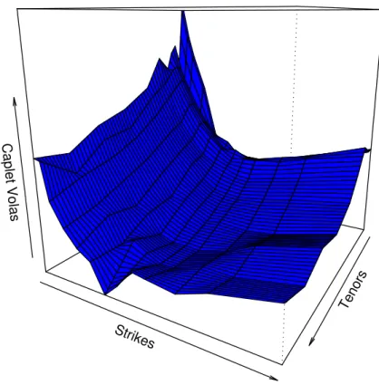
In this section we calibrate the model (4.3)–(4.5) to two caplet-strike volatility matrices available at the market on 19.06.2008 and 26.06.2008 respectively, which are partially shown in Tables 1, 2. A corresponding implied volatility surface is shown in Figure 1, where smiles are clearly observable. Due to the structure of the given data sets we consider a Libor model based on semi-annual tenors, i.e.δj ≡ 0.5, withn = 41 (20
years).
In a pre-calibration a standard market model is calibrated to ATM caps and ATM swaptions using Schoenmakers (2005). However, we emphasize that the method by which this input market model is obtained is not essential nor considered a discussion
T/K 2.00 3.00 4.00 5.00 6.00 8.00 1 0.325 0.244 0.19 0.165 0.174 0.22 1.5 0.372 0.295 0.237 0.196 0.198 0.223 2 0.374 0.299 0.246 0.208 0.205 0.224 3 0.347 0.283 0.241 0.213 0.205 0.212 4 0.325 0.266 0.228 0.204 0.196 0.201 5 0.307 0.252 0.217 0.196 0.189 0.192 6 0.294 0.241 0.208 0.189 0.182 0.184 7 0.283 0.232 0.201 0.183 0.176 0.176 8 0.274 0.225 0.194 0.177 0.17 0.169 9 0.267 0.219 0.189 0.172 0.164 0.162 10 0.262 0.215 0.184 0.167 0.159 0.156 12 0.251 0.206 0.177 0.16 0.151 0.147 15 0.238 0.195 0.167 0.151 0.142 0.137 20 0.226 0.184 0.157 0.141 0.133 0.13 Table 1. Subset out of 195 caplet volatilitiesσK
T(in %) for different strikes and different tenor dates (in years), 19.06.2008.
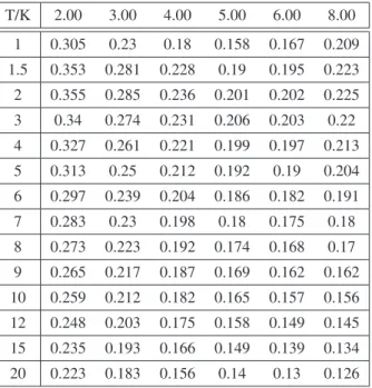
T/K 2.00 3.00 4.00 5.00 6.00 8.00 1 0.305 0.23 0.18 0.158 0.167 0.209 1.5 0.353 0.281 0.228 0.19 0.195 0.223 2 0.355 0.285 0.236 0.201 0.202 0.225 3 0.34 0.274 0.231 0.206 0.203 0.22 4 0.327 0.261 0.221 0.199 0.197 0.213 5 0.313 0.25 0.212 0.192 0.19 0.204 6 0.297 0.239 0.204 0.186 0.182 0.191 7 0.283 0.23 0.198 0.18 0.175 0.18 8 0.273 0.223 0.192 0.174 0.168 0.17 9 0.265 0.217 0.187 0.169 0.162 0.162 10 0.259 0.212 0.182 0.165 0.157 0.156 12 0.248 0.203 0.175 0.158 0.149 0.145 15 0.235 0.193 0.166 0.149 0.139 0.134 20 0.223 0.183 0.156 0.14 0.13 0.126 Table 2. Subset out of 195 caplet volatilitiesσK
T(in %) for different strikes and different tenor dates (in years), 26.06.2008.
Tenors Strikes
Caplet Volas
Figure 1. Caplet implied volatility surfaceσK
T.
point for this paper. For the pre-calibration we have used a volatility structure of the form
γi(t) =cig(Ti−t)ei+1−m(t), 0< t≤Ti, 1≤i < n,
where g is a simple parametric function, ei are unit vectors, and m(t)is defined in
(3.6). The pre-calibration routine returnsei∈Rn−1such that(ei,k)is upper triangular
and e⊤i ej=ρij = exp −|j−i| m−1(−lnρ∞ (7.1) −ηi 2+j2+ij −mi−mj−3i−3j+3m+2 (m−2)(m−3) , i, j=1, . . . , m:=n−1, 0≤η≤ −lnρ∞.
The functiongis parameterized as
For the Libor market model the loading factorsciare readily computed from (σAT M Ti ) 2T i =c2i Z Ti 0 g2(s)ds, i=1, . . . , n−1. (7.3) The initial Libor curve, is directly obtained from present values given at the respective calibration dates and (partially) given in Table 3.
Calibrating the market model
The market model calibration is based on an objective function which involves the squared distance between a set of market and model swaption volatilities, and a term which penalizes the deviationPi(ci−ci+1)2from being constant, where thecis are
computed from (7.3) (see also Section 3.2 for a motivation). For the respective dates Table 4 shows the parameters for the scalar volatility function (7.2) and correlation matrix (7.1) based on a calibration of the market model to 93 swaption quotes. These scalar volatility functions and correlation structures are taken as inputs for the stochas-tic volatility model while the constantsciwill be calibrated newly for flexibility. The
results of the calibration of the multiple stochastic volatility model to the cap-strike matrix at the respective calibration dates are given in Tables 5, 6. We note that the stochastic volatility calibration is done with respected option prices (rather than volatil-ities as usual when calibrating a market model).
Comments on the calibration
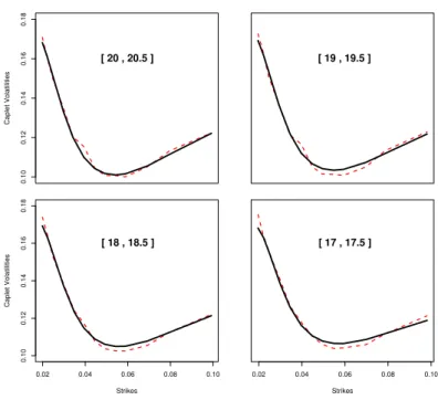
It turned that for these data sets the stochastic volatility parameter r needed to be taken rather close to one,r ≡ 0.9.A qualitative impression of the calibration can be obtained from Figure 2. From the last down to the sixed tenor the relative average price calibration fit is about 5% for both data sets. For the short term tenors (up to the fifth) the calibration errors growth up to about 13%–25% unfortunately, and are therefore not reported. We found out however that the main reason for this bad fit for small maturities is the erratic behavior of the yield curve over this period at the calibration dates (see Table 3). For instance after replacing the actual yield curve with a smoothed one we also got a good fit for small maturities. The overall relative root-mean-square fit we have reached shows to be 0.5%–5%, when the caplet maturity ranges from 0.5 to 20.
Regarding computation time we can say that an overall calibration to 40 tenors each involving 10 strikes takes about 7 minutes on a nowadays usual notebook (Pentium-III). Moreover, to the best of our knowledge, we are not aware of any stochastic volatil-ity model which is able to produce a comparable fit in less or comparable computation time, to a system of cap-strike matrices over such a wide range of tenors.
Ti Li(0)19.06.08 Li(0)26.06.08 Ti Li(0)19.06.08 Li(0)26.06.08 0.5 0.0582 0.0587 10.5 0.0500 0.0516 1 0.0665 0.0669 11 0.0500 0.0520 1.5 0.0514 0.0500 11.5 0.0502 0.0522 2 0.0390 0.0368 12 0.0504 0.0523 2.5 0.0476 0.0461 12.5 0.0503 0.0520 3 0.0557 0.0561 13 0.0502 0.0520 3.5 0.0517 0.0520 13.5 0.0502 0.0521 4 0.0472 0.0471 14 0.0501 0.0521 4.5 0.0475 0.0477 14.5 0.0500 0.0518 5 0.0481 0.0488 15 0.0498 0.0517 5.5 0.0474 0.0485 15.5 0.0496 0.0517 6 0.0466 0.0484 16 0.0494 0.0515 6.5 0.0473 0.0488 16.5 0.0491 0.0510 7 0.0477 0.0493 17 0.0489 0.0508 7.5 0.0480 0.0497 17.5 0.0488 0.0509 8 0.0484 0.0500 18 0.0487 0.0508 8.5 0.0489 0.0504 18.5 0.0485 0.0503 9 0.0493 0.0508 19 0.0482 0.0498 9.5 0.0497 0.0511 19.5 0.0479 0.0495 10 0.0499 0.0514 20 0.0476 0.0493
Table 3. Initial Libor curves
19.06.08 26.06.08 η 0.007 0.010 ρ∞ 0.101 0.100 a 5.001 5.000 b 2.000 2.001 g∞ 2.578 2.213
Table 4. LMM parameters for correlation structure and volatility function from calibration to ATM caplets.
Libori ρi σi κi ci rel. price err. (%) 40 −0.8 1.697 1.444 3.133 5.5 39 −0.8 1.671 1.444 2.908 5.8 38 −0.8 1.691 1.444 2.861 5.7 37 −0.8 1.691 1.444 2.82 6.1 36 −0.8 1.691 1.444 2.774 5.4 35 −0.8 1.635 1.444 2.56 5.8 34 −0.8 1.683 1.444 2.495 5.8 33 −0.8 1.697 1.444 2.456 5.4 32 −0.8 1.697 1.444 2.415 6 31 −0.8 1.697 1.444 2.378 5.3 30 −0.8 1.697 1.444 2.193 5.6 29 −0.8 1.681 1.444 2.15 5.4 28 −0.8 1.694 1.444 2.245 5.4 27 −0.8 1.694 1.444 2.185 5.3 26 −0.8 1.694 1.444 2.118 5.3 25 −0.8 1.694 1.444 2.056 5 24 −0.8 1.694 1.444 1.994 5 23 −0.8 1.694 1.444 1.908 5.1 22 −0.8 1.655 1.444 1.828 4.8 21 −0.8 1.668 1.444 1.648 5 20 −0.8 1.691 1.444 1.572 5.2 19 −0.8 1.691 1.444 1.567 4.7 18 −0.8 1.656 1.444 1.477 4.9 17 −0.8 1.691 1.444 1.398 5.1 16 −0.8 1.43 1.444 1.375 5.1 15 −0.8 1.699 1.444 1.297 5.2 14 −0.8 1.677 1.444 1.22 4.8 13 −0.8 1.511 1.444 1.202 6.3 12 −0.8 1.656 1.444 1.125 6.2 11 −0.8 1.648 1.444 1.091 6.6 10 −0.8 1.593 1.444 1.014 7 9 −0.8 1.696 1.444 0.937 7.1 8 −0.8 1.301 1.444 0.923 8.8 7 −0.8 1.576 1.444 0.91 5.5 6 −0.8 2.245 5.87 0.956 6 5 −0.8 2.905 5.87 0.869 12.4
Libori ρi σi κi ci rel. price err. (%) 40 −0.8 2.002 2.008 2.029 5.5 39 −0.8 1.971 2.008 2.001 5.4 38 −0.8 1.93 2.008 1.86 5.5 37 −0.8 1.999 2.008 2.032 5.3 36 −0.8 1.999 2.008 1.91 5.2 35 −0.8 1.999 2.008 1.881 4.9 34 −0.8 1.962 2.008 1.82 5 33 −0.8 1.943 2.008 1.8 4.6 32 −0.8 1.964 2.008 1.71 4.9 31 −0.8 1.951 2.008 1.668 4.6 30 −0.8 1.997 2.008 1.594 4.6 29 −0.8 1.981 2.008 1.558 4.5 28 −0.8 1.906 2.008 1.53 4.3 27 −0.8 1.874 2.008 1.487 4.2 26 −0.8 2.004 2.008 1.434 4.1 25 −0.8 1.991 2.008 1.394 4 24 −0.8 1.935 2.008 1.36 4 23 −0.8 2.004 2.008 1.325 3.8 22 −0.8 2.004 2.008 1.262 3.8 21 −0.8 1.878 2.008 1.233 3.4 20 −0.8 2.004 2.008 1.203 3.5 19 −0.8 1.983 2.008 1.145 3.8 18 −0.8 1.997 2.008 1.087 4 17 −0.8 1.997 2.008 1.039 4.1 16 −0.8 1.997 2.008 1.039 4.2 15 −0.8 1.915 2.008 0.949 3.9 14 −0.8 4.002 8.042 0.949 5.4 13 −0.8 3.873 8.042 0.899 5.9 12 −0.8 3.826 8.042 0.897 6.7 11 −0.8 3.695 8.042 0.839 6.3 10 −0.8 3.3 8.042 0.732 7.9 9 −0.8 3.549 8.042 0.737 7.5 8 −0.8 3.549 8.042 0.68 9.8 7 −0.8 3.952 11.125 0.753 7.9 6 −0.8 3.704 13.065 0.737 5.2 5 −0.8 4.914 16.902 0.705 14
0.10 0.12 0.14 0.16 0.18 Caplet Volatilities [ 20 , 20.5 ] [ 19 , 19.5 ] 0.02 0.04 0.06 0.08 0.10 0.10 0.12 0.14 0.16 0.18 Strikes Caplet Volatilities [ 18 , 18.5 ] 0.02 0.04 0.06 0.08 0.10 Strikes [ 17 , 17.5 ]
Figure 2. Caplet volas from the calibrated model (solid lines) and market caplets volasσK T (dashed lines) for different caplet periods.
Concluding remarks
We have proposed an economically motivated multiple stochastic volatility extension of a given (pre-calibrated) Libor market model which is suited for Monte Carlo sim-ulation of exotic interest rate products. Also it is shown that this extension allows for fast (approximative) cap and swaption pricing with smiles which enables efficient cal-ibration to these products. A road map for calcal-ibration to the cap-strike matrix is given and illustrated by a case study. The considered data sets in this study were taken at rather turbulent times, to reveal some stress issues of the model calibration. We just note that by considering more smooth data sets (smooth yield curves in particular), it is observed that the calibration performs overall satisfactory. Finally, we underline that in this paper the main focus is on the structure of the presented stochastic volatil-ity model and its implementation. An in-depth analysis of the model calibration and enhancements of the calibration procedure on an engineering level may be considered. In fact, this is part of recent research related to industrial cooperation projects. Further, calibration to other products such as CMS-spreads may be interesting (see for instance Belomestny, Kolodko, Schoenmakers (2008)).
8. Appendix
8.1. The Conditional Characteristic Function
Forj =1, . . . , n−1, we need to determine the characteristic function of lnLj(T)−
lnLj(0)under the relevant measurePj+1. For each componentk=1, . . . , n−1, the Heston CIR-process has the general form
dvk =κ( j+1) k (θ (j+1) k −vk)dt+σkρk √ vkdfW( j+1) k +σk q (1−ρ2k)√vkdW (j+1) k .
For a forward Libor dynamic given by (5.5) with initialv∈Rn−1, it then follows that the characteristic function is given by
ϕj+1(z;T, v) =Ej+1 " eizln Lj(T) Lj(0) vk(0) =vk, k=1, . . . , n−1 # =ϕj+1,0(z;T) nY−1 k=j ϕj+1,k(z;T, vk), (8.1) where ϕj+1,0(z;T) =exp −12(1−r2)η2j(T) z2+iz , ηj2(T) = Z T 0 |γj| 2 dt, and for each fixedk,ϕj+1,k(z;T, vk):= bpj+1,k(z;T, yk, vk)yk=0withpbj+1,k
satis-fying the parabolic equation ∂pbj+1,k ∂T =κ (j+1) k (θ (j+1) k −vk) ∂pbj+1,k ∂vk − 1 2r 2γ2 jkvk ∂pbj+1,k ∂yk +1 2σ 2 kvk ∂2pbj+1,k ∂vk2 + 1 2r 2γ2 jkvk ∂2pbj+1,k ∂yk2 +σkρkrγjkvk ∂2pbj+1,k ∂yk∂vk
with boundary condition
b
pj+1,k(z; 0, yk, vk) =e
izyk.
This can be easily verified by the Feynman–Kac formula. It is well known that the above equation can be solved explicitly by the ansatz
b
pj+1,k(z;T, yk, vk) =exp(Aj,k(z;T) +vkBj,k(z;T) +izyk),
which yields a Riccati equation inAj,kandBj,kwith solution
Aj,k(z;T) = κ(kj+1)θk(j+1) σk2 (aj,k−dj,k)T −2 ln e−dj,kT −g j,k 1−gj,k , Bj,k(z;T) = (aj,k+dj,k)(1−edj,kT) σk2(1−gj,kedj,kT) , (8.2)
where aj,k=κ (j+1) k −irρkσkγjkz, dj,k= q a2j,k+r2γ2 jkσk2(z2+iz), gj,k= aj,k+dj,k aj,k−dj,k . We thus obtain ϕj+1,k(z;T, vk) =exp(Aj,k(z;T) +vkBj,k(z;T)).
In (8.2) we have chosen the formulation of Lord and Kahl (2005) which has the conve-nient property that we can take in (8.2) for the complex logarithm always the principle branch. Note that the lower indexj+1 in the characteristic function refers to the mea-sure, whereas the indexj in the introduced coefficients refers to the relevant forward Libor. The second index krefers to the component. It is again the choice ofγ that enables the product in (8.1) to be started at j. This crucial feature will show to be beneficial in the calibration part. Whenj =n−1, for example, only the last log-Libor will contribute a non-trivial factor to the characteristic function. For all others we have ϕn,k ≡1, k=1, . . . , n−2.
8.2. CIR
Consider a CIR model of the form,
dv(t) =κ(θ−v(t))dt+σpv(t)dW(t), κ, θ, σ >0. Givenv(u),v(t)witht > uis distributed with density
νχ2d(νx, ξ)
whereχ2d(x, ξ)is the density of a noncentral chi-square random variable withddegrees of freedom and noncentrality parameterξand
ν= 4κ σ2(1−e−κ(t−u)), ξ= 4κe −κ(t−u) σ2(1−e−κ(t−u))v(u), d= 4θκ σ2 . The conditional mean ofv(t)is given by
E(v(t)|v(u)) =ν−1(ξ+d) = (v(u)
and the conditional second moment is E(v2(t)|v(u)) = (2(d+2ξ) + (ξ+d) 2) ν2 = 1+2 d [E(v(t)|v(u))]2− 2 de −2κ(t−u)v2(u). 8.3. Measure invariance
Why isdW(kn,i+1)invariant under the various measures?
See Jamshidian for the compensator, which is given by µi+1 W(kn) =hW (n) k ,lnMi with M =Πnj=−i1+1(1+δjLj).
That is, we have
hW(kn),lnMi=dW (n) k dlnM =dW (n) k d n−1 X j=i+1 ln(1+δjLj) = n−1 X j=i+1 dW(kn)dln(1+δjLj) = n−1 X j=i+1 δjLj 1+δjLj dW(kn)dlnLj.
A closer look at (4.1) reveals that all terms are negligible, since of higher order than dt, or zero due to independence ofWandW orfW, respectively. We thus have
hW(kn),lnMi=0
or in other words, as indicated bydW(kn,i+1):
dW(kn)=dW
(i+1)
k .
Analogously we obtain by exchangingWkwithWfkthat
= n−1 X j=i+1 δjLj 1+δjLj dfWk(n)dlnLj = n−1 X j=i+1 rδjLj 1+δjLj βjk q vk tdt.
Acknowledgments.Partial support by the Deutsche Forschungsgemeinschaft through the SFB 649 ‘Economic Risk’ and the DFG Research Center MATHEON‘Mathematics
for Key Technologies’ in Berlin is gratefully acknowledged. We thank Rohit Saraf (Columbia University) for a useful remark.
References
1. Andersen, L. and R. Brotherton-Ratcliffe (2005). Extended Libor Market Models with Stochastic Volatility.Journal of Computational Finance,9, no. 1, 1–40.
2. Andersen, L. and Piterbarg, V. (2007). Moment Explosions in Stochastic Volatility Mod-els.Finance and Stochastics,11, no. 1, 29–50.
3. Belomestny, D., Kampen, J. and J. Schoenmakers (2009). Holomorphic transforms with application to affine processes.Journal of Functional Analysis,no. 257, 1222–1250. 4. Belomestny, D., Kolodko, A. and J. Schoenmakers (2008). Pricing CMS spreads in the
Libor market model. WIAS preprint 1386.
5. Belomestny, D. and M. Reiß (2006). Optimal calibration of exponential Lévy models. Finance and Stochastics,10, no. 4, 449–474.
6. Belomestny, D. and J.G.M. Schoenmakers (2006). A Jump-Diffusion Libor Model and its Robust Calibration. WIAS preprint 1113,Quantitative Finance,to appear.
7. Brigo, D. and F. Mercurio (2001). Interest rate models–theory and practice. Springer-Verlag, Berlin.
8. Brace, A., Gatarek, D. and M. Musiela (1997). The Market Model of Interest Rate Dy-namics.Mathematical Finance,7, no. 2, 127–155.
9. Carr, P. and D. Madan (1999). Option Valuation Using the Fast Fourier Transform.Journal of Computational Finance,2, 61–74.
10. Cox, J.C., Ingersoll, J.E. and S.A. Ross (1985). A Theory of the Term Structure of Interest Rates.Econometrica53, 385–407.
11. Eberlein, E., Keller U. and K. Prause (1998). New insights into smile, mispricing, and value at risk: the hyperbolic model.Journal of Business,71, no. 3, 371–405.
12. Eberlein, E. and F. Özkan (2005). The Lévy Libor model, Finance and Stochastics7, no. 1, 1–27.
13. Glasserman, P. (2004).Monte Carlo methods in financial engineering. Springer-Verlag, New York.
14. Glasserman, P. and S.G. Kou (2003). The term structure of simple forward rates with jump risk.Mathematical Finance13, no. 3, 383–410.
15. Hagan, P. S., Kumar, D., Lesniewski, A. S. and D. E. Woodward (2002). Managing smile risk. WILMOTT Magazine September, 84–108.
16. Heston, S. (1993). A closed-form solution for options with stochastic volatility with appli-cations to bond and currency options.The Review of Financial Studies,6, no. 2, 327–343. 17. Jamshidian, F.(1997). LIBOR and swap market models and measures. Finance and
Stochastics,1, 293–330.
18. Jamshidian, F.(2001). LIBOR Market Model with Semimartingales. In “Option Pricing, Interest Rates and Risk Management”, Cambridge Univ. Press.
19. Kahl Ch. and P. Jäckel (2006). Fast strong approximation Monte Carlo schemes for stochastic volatility models.Quantitative Finance,6, no. 6, 513–536.
20. Lord R. and C. Kahl (2005). Complex logarithms in Heston-like models.Mathematical Finance,to appear.
21. Mercurio F. and M. Morini (2007). No-arbitrage dynamics for a tractable SABR term structure Libor Model. SSRN Working Paper.
22. Merton, R.C. (1976). Option pricing when underlying stock returns are discontinuous.J. Financial Economics,3, no. 1, 125–144.
23. Miltersen, K., K. Sandmann, and D. Sondermann (1997). Closed-form solutions for term structure derivatives with lognormal interest rates.Journal of Finance,52, 409–430. 24. Piterbarg, V. (2004). A stochastic volatility forward Libor model with a term structure of
volatility smiles. SSRN Working Paper.
25. Piterbarg, V. (2005). Is CMS spread volatility sold too cheap? Presented at II Fixed Income Conference, Prague.
26. Schoenmakers, J. (2005).Robust Libor Modelling and Pricing of Derivative Products. BocaRaton London NewYork Singapore: Chapman & Hall–CRC Press.
27. Wu, L. and F. Zhang (2006). Libor Market Model with Stochastic Volatility.Journal of Industrial and Management Optimization,2, 199–207.
28. Zhu, J. (2007). An extended Libor Market Model with nested stochastic volatility dynam-ics. SSRN Working Paper.
Received February 19, 2009; revised October 2, 2009
Author information
Denis Belomestny, Weierstrass Institute for Applied Analysis and Stochastics, Mohrenstr. 39, 10117 Berlin, Germany.
Email:[email protected]
Stanley Mathew, Johann Wolfgang Goethe-Universität, Senckenberganlage 31, 60325 Frank-furt am Main, Germany.
Email:[email protected]
John Schoenmakers, Weierstrass Institute for Applied Analysis and Stochastics, Mohrenstr. 39, 10117 Berlin, Germany.