SFB 649 Discussion Paper 2010-002
Partial Linear Quantile
Regression and
Bootstrap Confidence Bands
Wolfgang Karl Härdle*
Ya’acov Ritov**
Song Song*
* Humboldt-Universität zu Berlin, Germany ** Hebrew University of Jerusalem, Israel
This research was supported by the Deutsche
Forschungsgemeinschaft through the SFB 649 "Economic Risk". http://sfb649.wiwi.hu-berlin.de ISSN 1860-5664 SFB 649, Humboldt-Universität zu Berlin
S
FB
6
49
E
C
O
N
O
M
I
CR
I
SK
B
ER
L
I
N
Partial Linear Quantile Regression and
Bootstrap Confidence Bands
∗
Wolfgang K. H¨
ardle
†, Ya’acov Ritov
‡, Song Song
§November 28, 2009
Abstract
In this paper uniform confidence bands are constructed for non-parametric quantile estimates of regression functions. The method is based on the bootstrap, where resampling is done from a suitably estimated empirical density function (edf) for residuals. It is known that the approximation error for the uniform confidence band by the asymptotic Gumbel distribution is logarithmically slow. It is proved that the bootstrap approximation provides a substantial improvement. The case of multidimensional and discrete regressor variables is dealt with using a partial linear model. Comparison to classic asymptotic uniform bands is presented through a simulation study. An economic application considers the labour market differential effect with respect to different education levels.
Keywords: Bootstrap, Quantile Regression, Confidence Bands, Non-parametric Fitting, Kernel Smoothing, Partial Linear Model
JEL classification: C14; C21; C31; J01; J31; J71
∗The financial support from the Deutsche Forschungsgemeinschaft via SFB 649
“ ¨Okonomisches Risiko”, Humboldt-Universit¨at zu Berlin is gratefully acknowledged. Ya’acov Ritov’s research is supported by an ISF grant and a Humboldt Award. We thank Thorsten Vogel and Alexandra Spitz-Oener for sharing their data / comments and suggestions.
†Professor at Humboldt-Universit¨at zu Berlin and Director of C.A.S.E. - Center for
Applied Statistics and Economics, Humboldt-Universit¨at zu Berlin, Berlin, Germany. & Department of Finance, National Central University, Taipei, Taiwan, R.O.C.
‡Professor at The Hebrew University of Jerusalem, Department of Statistics and the
Center for the Study of Rationality, Jerusalem, Israel.
§Corresponding author. Research associate at the Institute for Statistics and
Econo-metrics of Humboldt-Universit¨at zu Berlin, Spandauer Straße 1, 10178 Berlin, Germany. Email: [email protected].
1
Introduction
Quantile regression, as first introduced by Koenker and Bassett (1978), is “gradually developing into a comprehensive strategy for completing the re-gression prediction” as claimed by Koenker and Hallock (2001). Quantile smoothing is an effective method to estimate quantile curves in a flexible nonparametric way. Since this technique makes no structural assumptions on the underlying curve, it is very important to have a device for understand-ing when observed features are significant and decidunderstand-ing between functional forms, for example a question often asked in this context is whether or not an observed peak or valley is actually a feature of the underlying regression function or is only an artifact of the observational noise. For such issues, confidence intervals should be used that are simultaneous (i.e., uniform over location) in nature. Moreover, uniform confidence bands give an idea about the global variability of the estimate.
In the previous work the theoretical focus has mainly been on obtain-ing consistency and asymptotic normality of the quantile smoother, thereby providing the necessary ingredients to construct its pointwise confidence in-tervals. This, however, is not sufficient to get an idea about the global vari-ability of the estimate, neither can it be used to correctly answer questions about the curve’s shape, which contains the lack of fit test as an immediate application. This motivates us to construct the confidence bands. To this end, H¨ardle and Song (2010) used strong approximations of the empirical process and extreme value theory. However, the very poor convergence rate of extremes of a sequence of n independent normal random variables is well documented and was first noticed and investigated by Fisher and Tippett (1928), and discussed in greater detail by Hall (1991). In the latter paper it was shown that the rate of the convergence to its limit (the suprema of a stationary Gaussian process) can be no faster than (logn)−1. For example, the supremum of a nonparametric quantile estimate can converge to its limit no faster than (logn)−1. These results may make extreme value approxi-mation of the distributions of suprema somewhat doubtful, for example in the context of the uniform confidence band construction for a nonparametric quantile estimate.
This paper proposes and analyzes a method of obtaining any number of uniform confidence bands for quantile estimates. The method is simple to implement, does not rely on the evaluation of quantities which appear in asymptotic distributions and also takes the bias properly into account (at least asymptotically). More importantly, we show that the bootstrap approximation to the distribution of the supremum of a quantile estimate is accurate to within n−2/5 which represents a significant improvement relative
to (logn)−1. Previous research by Hahn (1995) showed consistency of a bootstrap approximation to the cumulative density function (cdf) without assuming independence of the error and regressor terms. Horowitz (1998) showed bootstrap methods for median regression models based on a smoothed least-absolute-deviations (SLAD) estimate.
Let (X1, Y1), (X2, Y2), . . ., (Xn, Yn) be a sequence of independent
identi-cally distributed bivariate random variables with joint pdf f(x, y), joint cdf
F(x, y), conditional pdf f(y|x), f(x|y), conditional cdfF(y|x),F(x|y) for Y
given X and X given Y respectively, and marginal pdf fX(x) for X, fY(y)
forY. With some abuse of notation we use the lettersf andF to denote dif-ferent pdf’s and cdf’s respectively. The exact distribution will be clear from the context. At the first stage we assume that x ∈ J∗, and J∗ = (a, b) for some 0< a < b <1. Letl(x) denote thep-quantile curve, i.e. l(x) = FY−|1x(p). In economics, discrete or categorial regressors are very common. An ex-ample is from labour market analyse where one tries to find out how revenues depend on the age of the employee (for different education levels, labour union status, genders and nationalities), i.e. in econometric analysis one targets for the differential effects. For example, Buchinsky (1995) examined the U.S. wage structure by quantile regression techniques. This motivates the extension to multivariate covariables by partial linear modelling (PLM). This is convenient especially when we have categorial elements of the X vec-tor. Partial linear models, which were first considered by Green and Yandell (1985), Denby (1986), Speckman (1988) and Robinson (1988), are gradually developing into a class of commonly used and studied semiparametric regres-sion models, which can retain the flexibility of nonparametric models and ease the interpretation of linear regression models while avoiding the “curse of dimensionality”. Recently Liang and Li (2009) used penalised quantile regression for variable selection of partially linear models with measurement errors.
In this paper, we propose an extension of the quantile regression model to x = (u, v)> ∈ Rd with u ∈
Rd−1 and v ∈ J∗ ⊂ R. The quantile
re-gression curve we consider is: ˜l(x) = FY−|1x(p) = u>β +l(v). The multi-variate confidence band can now be constructed, based on the unimulti-variate uniform confidence band, plus the estimated linear part which we will prove is more accurately (√n consistency) estimated. This makes various tasks in economics, e.g. labour market differential effect investigation, multivariate model specification tests and the investigation of the distribution of income and wealth across regions, countries or the distribution across households possible. Additionally, since the natural link between quantile and expec-tile regression was developed by Newey and Powell (1987), we can further extend our result into expectile regression for various tasks, e.g.
demog-raphy risk research or expectile-based Value at Risk (EVAR) as in Kuan et al. (2009). For high-dimensional modelling, Belloni and Chernozhukov (2009) recently investigated high-dimensional sparse models with L1 penalty (LASSO). Additionally, by simple calculations, our result can be further ex-tended to intersection bounds (one side confidence bands), which is similar to Chernozhukov et al. (2009).
The rest of this article is organised as follows. To keep the main idea transparent, we start with Section 2, as an introduction to the more compli-cated situation, the bootstrap approximation rate for the uniform confidence band (univariate case) in quantile regression is presented through a coupling argument. An extension to multivariate covariance X with partial linear modelling is shown in Section 3 with the actual type of confidence bands and their properties. In Section 4, in the Monte Carlo study we compare the bootstrap uniform confidence band with the one based on the asymptotic theory and investigate the behaviour of partial linear estimates with the cor-responding confidence band. In Section 5, an application considers the labour market differential effect. The discussion is restricted to the semiparamet-ric extension. We do not discuss the general nonparametsemiparamet-ric regression. We conjecture that this extension is possible under appropriate conditions. All proofs are sketched in Section 6.
2
Bootstrap confidence bands in the
univari-ate case
Suppose Yi = l(Xi) +εi, i = 1, . . . , n, where εi has distribution function F(·|Xi). For simplicity, but without any loss of generality, we assume that F(0|Xi) = p. F(ξ|x) is smooth as a function of x and ξ for any x, and for
any ξ in the neighbourhood of 0. We assume:
(A1). X1, . . . , Xnare an i.i.d. sample, and infxfX(x) =λ0 >0. The quantile function satisfies: supx|l(j)(x)| ≤λj <∞, j = 1,2.
(A2). The distribution ofY givenX has a density and infx,tf(t|x)≥λ3 >0, continuous in x, and in t in a neighbourhood of 0. More exactly, we have the following Taylor expansion, for some A(·) and f0(·), and for every x, x0, t: F(t|x0) = p+f0(x)t+A(x)(x0−x) +R(t, x0;x), (1) where sup t,x,x0 |R(t, x0;x)| t2+|x0−x|2 <∞.
Let K be a symmetric density function with compact support and dK =
R
u2K(u)du < ∞. Let l
h(·) = ln,h(·) be the nonparametric p-quantile
es-timate of Y1, . . . , Yn with weight function K{(Xi − ·)/h} for some global
bandwidth h=hn (Kh(u) =h−1K(u/h)), that is, a solution of:
Pn i=1Kh(x−Xi)1{Yi < lh(x)} Pn i=1Kh(x−Xi) < q ≤ Pn i=1Kh(x−Xi)1{Yi ≤lh(x)} Pn i=1Kh(x−Xi) . (2) Generally, the bandwidth may also depend on x. A local (adaptive) band-width selection though deserves future research.
Note that by assumption (A1),lh(x) is the quantile of a discrete
distribu-tion, which is equivalent to a sample of sizeOp(nh) from a distribution withp
-quantile whose bias isO(h2) relative to the true value. Letδnbe the local rate
of convergence of the function lh, essentially δn =h2+ (nh)−1/2 = O(n−2/5)
with optimal bandwidth choice h = hn = O(n−1/5). We employ also an
auxiliary estimate lg
def
= ln,g, essentially one similar toln,h but with a slightly
larger bandwidth g = gn = hnnζ (a heuristic explanation of why it is
es-sential to oversmooth g is given later), whereζ is some small number. The asymptotically optimal choice of ζ as shown later is 4/45.
(A3). The estimate lg satisfies:
sup x∈J∗ |lg00(x)−l00(x)| = Op(1), sup x∈J∗ |l0g(x)−l0(x)| = Op(δn/h). (3)
Assumption (A3) is only stated to overwrite the issue here. It actually follows from the assumptions on (g, h). A sequence{an}is slowly varying ifn−αan→
0 for any α > 0. With some abuse of notation we will use Sn to denote any
slowly varying function which may change from place to place e.g. S2
n =Sn
is a valid expression (since ifSnis a slowly varying function, thenSn2 is slowly
varying as well). λi and Ci are generic constants throughout this paper and
the subscripts have no specific meaning. Note that there is noSn term in (3)
exactly because the bandwidth gn used to calculate lg is slightly larger than
that used for lh. As a result lg, as an estimate of the quantile function, has
a slightly worse rate of convergence, but its derivatives converge faster. We also consider a family of estimates ˆF(·|Xi), i = 1, . . . , n, estimating
respectively F(·|Xi) and satisfying ˆF(0|Xi) = p. For example we can take
the distribution with a point mass c−1K{α
n(Xj −Xi)} on Yj −lh(Xi), j = 1, . . . , n, wherec=Pn j=1K{αn(Xj −Xi)} and αn≈h−1, i.e. ˆ F(·|Xi) = Pn j=1Kh(Xj −Xi)1{Yj −lh(Xi)≤ ·} Pn j=1Kh(Xj −Xi)
We additionally assume:
(A4). fX(x) is twice continuously differentiable andf(t|x) is uniformly bounded
in x and t by, say,λ4.
LEMMA 2.1 [Franke and Mwita (2003), p14] If assumptions (A1, A2, A4)
hold, then for any small enough (positive) ε→0,
sup
|t|<ε,i=1,...,n,Xi∈J∗
|Fˆ(t|Xi)−F(t|Xi)|=Op{Snδnε1/2+ε2}. (4)
Note that the result in Lemma 2.1 is natural, since by definition, there is no error at t = 0, since ˆF(0|Xi) ≡ p ≡ F(0|Xi). For t ∈ (0, ε), ˆF(t|Xi),
like lh, is based on a sample of size Op(nh). Hence, the random error is
Op{(nh)−1/2t1/2}, while the bias is Op(εh2) = Op(δn). The Sn term takes
care of the maximisation.
LetF−1(·|·) and ˆF−1(·|·) be the inverse function of the conditional cdf and its estimate. We consider the following bootstrap procedure: Let U1, . . . , Un
be i.i.d. uniform [0,1] variables. Let
Yi∗ =lg(Xi) + ˆF−1(Ui|Xi), i= 1, . . . , n (5)
be the bootstrap sample. We couple this sample to an unobserved hypothet-ical sample from the true conditional distribution:
Yi#=l(Xi) +F−1(Ui|Xi), i= 1, . . . , n. (6)
Note that the vectors (Y1, . . . , Yn) and (Y
#
1 , . . . , Yn#) are equally distributed
given X1, . . . , Xn. We are really interested in the exact values of Yi# and Yi∗ only when they are near the appropriate quantile, that is, only if |Ui− p| < Snδn. But then, by equation (1), Lemma 2.1 and the inverse function
theorem, we have: max i:|F−1(U i|Xi)−F−1(p)|<Snδn |F−1(Ui|Xi)−Fb−1(Ui|Xi)| = max i:|Yi#−l(Xi)|<Snδn |Yi#−l(Xi)−Yi∗+lg(Xi)|=Op{Snδn3/2}. (7)
Let now qhi(Y1, . . . , Yn) be the solution of the local quantile as given by
(2) at Xi, with bandwidth h, i.e. qhi(Y1, . . . , Yn)
def
= lh(Xi) for data set
{(Xi, Yi)}ni=1. Note that by (3), if |Xi−Xj|=O(h), then
max
|Xi−Xj|<ch
Letlh∗ andlh#be the local bootstrap quantile and its coupled sample analogue. Then lh∗(Xi)−lg(Xi) = qhi[{Yj∗−lg(Xi)}nj=1] = qhi[{Yj∗−lg(Xj) +lg(Xj)−lg(Xi)})nj=1], (9) while lh#(Xi)−l(Xi) =qhi[{Yj#−l(Xj) +l(Xj)−l(Xi)}nj=1]. (10) From (7) – (10) we conclude that
max
i |l
∗
h(Xi)−lg(Xi)−l#h(Xi) +l(Xi)|=Op(δn). (11)
Based on (11), we obtain the following theorem (the proof is given in the appendix):
THEOREM 2.1 If assumptions (A1 - A3) and Lemma 2.1 hold, then
sup
x∈J∗
|l∗h(x)−lg(x)−l#h(x) +l(x)|=Op(δn) = Op(n−2/5).
A number of replications ofl∗h(x) can be used as the basis for simultaneous error bars because the distribution of l#h(x)−l(x) is approximated by the distribution of lh∗(x)−lg(x), as Theorem 2.1 shows.
Although Theorem 2.1 is stated with a fixed bandwidth, in practice, to take care of the heteroscedasticity effect, we construct confidence bands with the width depending on the densities, which is motivated by the counterpart based on the asymptotic theory as in H¨ardle and Song (2010). Thus we have the following corollary:
COROLLARY 2.1 Under the assumptions (A1) - (A8), an approximate
(1−α)×100% confidence band over R is
lh(v) ± h ˆ f{lh(x)|x} q ˆ fX(x) i−1 d∗α,
whered∗α is based on the bootstrap sample (defined later) andfˆ{lh(x)|x}, fˆX(x)
are consistent estimators off{l(x)|x}, fX(x)with use off(y|x) =f(x, y)/fX(x).
Below is the summary of the basic steps for the bootstrap procedure: 1) Given (Xi, Yi), i= 1, . . . , n, compute the local quantile smoother lh(x)
ofY1, . . . , Ynwith bandwidthhand obtain residuals ˆεi =Yi−lh(Xi), i=
2) Compute the conditional edf: ˆ F(t|x) = Pn i=1Kh(x−Xi)1{εˆi 6t} Pn i=1Kh(x−Xi)
3) For each i = 1, . . . , n, generate random variables ε∗i,b ∼ Fˆ(t|x), b = 1, . . . , B and construct the bootstrap sample Yi,b∗, i = 1, . . . , n, b = 1, . . . , B as follows:
Yi,b∗ =lg(Xi) +ε∗i,b.
4) For each bootstrap sample {(Xi, Yi,b∗)}ni=1, compute l
∗
h and the random
variable db def = sup x∈J∗ h ˆ f{lh∗(x)|x} q ˆ fX(x)|lh∗(x)−lg(x)| i . (12)
where ˆf{l(x)|x}, fˆX(x) are consistent estimators of f{l(x)|x}, fX(x).
5) Calculate the (1−α) quantile d∗α of d1, . . . , dB.
6) Construct the bootstrap uniform confidence band centered aroundlh(x),
i.e. lh(x)± h ˆ f{lh(x)|x} q ˆ fX(x) i−1 d∗α.
While bootstrap methods are well-known tools for assessing variability, more care must be taken to properly account for the type of bias encountered in nonparametric curve estimation. The choice of bandwidth is crucial here. In our experience the bootstrap works well with a rather crude choice of g, one may, however, specify g more precisely. Since the main role of the pilot bandwidth is to provide a correct adjustment for the bias, we use the goal of bias estimation as a criterion. Recall that the bias in the estimation of l(x) by l#h(x) is given by
bh(x) =El#h(x)−l(x).
The bootstrap bias of the estimate constructed from the resampled data is ˆbh,g(x) =El∗
h(x)−lg(x). (13)
Note that in (13) the expected value is computed under the bootstrap estimation. The following theorem gives an asymptotic representation of the mean squared error for the problem of estimating bh(x) by ˆbh,g(x). It is then
straightforward to find g to minimise this representation. Such a choice ofg
will make the quantiles of the original and coupled bootstrap distributions close to each other. In addition to the technical assumptions before, we also need:
(A5). l and f are four times continuously differentiable. (A6). K is twice continuously differentiable.
THEOREM 2.2 Under assumptions (A1 - A6), for any x∈J∗
Eh nˆbh,g(x)−bh(x)
o2
|X1, . . . , Xn
i
∼h4(C1g4+C2n−1g−5) (14)
in the sense that the ratio between the RHS and the LHS tends in probability to 1 for some constants C1, C2.
An immediate consequence of Theorem 2.2 is that the rate of convergence of g should be n−1/9, see also H¨ardle and Marron (1991). This makes precise the previous intuition which indicated that g should slightly oversmooth. Under our assumptions, reasonable choices of h will be of the order n−1/5 as in Yu and Jones (1998). Hence, (14) shows once again that g should tend to zero more slowly than h. Note that Theorem 2.2 is not stated uniformly over h. The reason is that we are only trying to give some indication of how the pilot bandwidth g should be selected.
3
Bootstrap confidence bands in PLMs
The case of multivariate regressors may be handled via a semiparametric specification of the quantile regression curve. More specifically we assume that with x= (u, v)>∈Rd, v ∈
R:
˜l(x) =u>
β+l(v)
In this section we show how to proceed in this multivariate setting and how -based on Theorem 2.1 - a multivariate confidence band may be constructed. We first describe the numerical procedure for obtaining estimates of β and l, where l denotes - as in the earlier sections - the one-dimensional conditional quantile curve. We then move on to the theoretical properties. First note that the PLM quantile estimation problem can be seen as estimating (β, l) in
y = u>β+l(v) +ε (15) = ˜l(x) +ε
where the p-quantile of ε conditional on both u and v is 0.
In order to estimate β, let an denote an increasing sequence of positive
[0,1] for v in an intervals Ini, i = 1, . . . , an, of equal length bn and let mni
denote the midpoint of Ini. In each of these small intervalsIni, i= 1, . . . , an, l(v) can be considered as being approximately constant, and hence (15) can be considered as a linear model. This observation motivates the following two stage estimation procedure:
1) A linear quantile regression inside each partition is used to estimate ˆ
βi, i = 1, . . . , an. Their weighted mean yields ˆβ. More exactly,
con-sider the parametric quantile regression of y onu,1 v ∈[0, bn)
,1 v ∈ [bn,2bn) , . . . ,1 v ∈[1−bn,1]
. That is, let
ψ(t)def= (1−p)1(t <0) +p1(t >0). Then let ˆ β = arg min β min l1,...,lan n X i=1 ψ{Yi −βTUi− an X j=1 lj1 Vi ∈Ini }
2) Calculate the smooth quantile estimate as in (2) from (Vi, Yi−Ui>βˆ)ni=1, and name it as ˜˜lh(v).
The following theorem states the asymptotic distribution of ˆβ.
THEOREM 3.1 There exist positive definite matricesD, C (defined in the
appendix), such that √
n( ˆβ−β)→L N{0, p(1−p)D−1CD−1}asn → ∞.
Note thatl(v), ˜lh(v) (quantile smoother based on (v, y−u>β)) and ˜˜lh(v)
can be treated as a zero (w.r.t. θ, θ ∈ I where I is a possibly infinite, or possibly degenerate, interval in R) of the functions
e H(θ, v) def= Z R f(v,y˜)ψ(˜y−θ)dy,˜ (16) e Hn(θ, v) def = n−1 n X i=1 Kh(v−Vi)ψ(Yei−θ), (17) e e Hn(θ, v) def = n−1 n X i=1 Kh(v−Vi)ψ(Yeei−θ), (18)
where e Yi def = Yi−Ui>β e e Yi def = Yi−Ui>βˆ=Yi−Ui>β+U > i (β−βˆ) def = Yei+Zi.
From Theorem 3.1 we know that ˆβ−β =Op(1/
√
n) and||Zi||∞ =Op(1/
√
n). Under the following assumption, which are satisfied by exponential, and gen-eralised hyperbolic distributions, also used in H¨ardle et al. (1988):
(A7). The conditional densities f(·|y˜), y˜∈ R, are uniformly local Lipschitz continuous of order ˜α(ulL- ˜α) onJ, uniformly in ˜y∈R, with 0<α˜ 61, and (nh)/logn → ∞.
For some constant C3 not depending on n, Lemma 2.1 in H¨ardle and Song (2010) shows a.s. as n → ∞: sup θ∈I sup v∈J∗ |Hen(θ, v)−He(θ, v)| ≤ C3max{(nh/logn)−1/2, hα˜}.
Observing that ph/logn =O(1), we then have:
sup θ∈I sup v∈J∗ |e e Hn(θ, v)−He(θ, v)| ≤ sup θ∈I sup v∈J∗ |Hen(θ, v)−He(θ, v)| + sup θ∈I sup v∈J∗ |Hen(θ, v)−Heen(θ, v)| | {z } ≤Op(1/ √ n) supv∈J|n−1 P Kh| ≤ C4max{(nh/logn)−1/2, hα˜} (19) for a constant C4 which can be different from C3. To show the uniform consistency of the quantile smoother, we shall reduce the problem of strong convergence of ˜˜lh(v)−l(v), uniformly in v, to an application of the strong
convergence of e e
Hn(θ, v) to He(θ, v), uniformly in v and θ. For our result on
˜ ˜
lh(·), we shall also require
(A8). infv∈J∗
R
ψ{y−l(v) +ε}dF(y|v)>q˜|ε|, for|ε|6δ1,
where δ1 and ˜q are some positive constants, see also H¨ardle and Luckhaus (1984). This assumption is satisfied if a constant ˜q exists givingf{l(v)|v}>
˜
LEMMA 3.1 Under assumptions (A7) and (A8), we have a.s. as n → ∞
sup
v∈J∗
|˜˜lh(v)−l(v)| ≤C5max{(nh/logn)−1/2, hα˜} (20)
with another constant C5 not depending on n. If additionally ˜
α >{log(√logn)−log(√nh)}/logh, (20) can be further simplified to:
sup
v∈J∗
|˜˜lh(v)−l(v)| ≤C5{(nh/logn)−1/2}.
Since the proof is essentially the same as Theorem 2.1 of the above men-tioned reference, it is omitted here.
The convergence rate for the parametric partOp(n−1/2) (Theorem 3.1) is
smaller than the bootstrap approximation error for the nonparametric part
Op(n−2/5) as shown in Theorem 2.1. This makes the construction of uniform
confidence bands for multivariatex∈Rdwith a partial linear model possible.
PROPOSITION 3.1 Under the assumptions (A1) - (A8), an approximate
(1−α)×100% confidence band over Rd−1×[0,1] is
u>βˆ+lh(v) ± h ˆ f{lh(x)|x} q ˆ fX(x) i−1 d∗α,
where fˆ{lh(x)|x}, fˆX(x) are consistent estimators of f{l(x)|x}, fX(x).
4
A Monte Carlo study
This section is divided into two parts. First we concentrate on a univariate regressor variable x, check the validity of the bootstrap procedure together with settings in the specific example, and compare it with asymptotic uni-form bands. Secondly we incorporate the partial linear model to handle the multivariate case of x∈Rd.
Below is the summary of the simulation procedure:
1) Simulate (Xi, Yi), i= 1, . . . , naccording to their joint pdf f(x, y).
In order to compare with earlier results in the literature, we choose the joint pdf of bivariate data {(Xi, Yi)}ni=1, n= 1000 as:
f(x, y) =fy|x(y−sinx)1(x∈[0,1]), (21)
where fy|x(x) is the pdf of N(0, x) with an increasing heteroscedastic
structure. Thus the theoretical quantile is l(x) = sin(x) +√xΦ−1(p). Based on this normality property, all the assumptions can be seen to be satisfied.
2) Compute the local quantile smoother lh(x) of Y1, . . . , Yn with
band-width h and obtain residuals ˆεi =Yi−lh(Xi), i= 1, . . . , n.
If we choose p= 0.9, then Φ−1(p) = 1.2816, l(x) = sin(x) + 1.2816√x. Set h = 0.05.
3) Compute the conditional edf: ˆ F(t|x) = Pn i=1Kh(x−Xi)1{εˆi 6t} Pn i=1Kh(x−Xi) with the quartic kernel
K(u) = 15 16(1−u
2)2, (|u|
61).
4) For each i = 1, . . . , n, generate random variables ε∗i,b ∼ Fˆ(t|x), b = 1, . . . , B and construct the bootstrap sample Yi,b∗, i = 1, . . . , n, b = 1, . . . , B as follows:
Yi,b∗ =lg(Xi) +ε∗i,b,
with g = 0.2.
5) For each bootstrap sample {(Xi, Yi,b∗)}ni=1, compute lh∗ and the random
variable db def = sup x∈J∗ h ˆ f{lh∗(x)|x} q ˆ fX(x)|lh∗(x)−lg(x)| i . (22)
where ˆf{l(x)|x}, fˆX(x) are consistent estimators of f{l(x)|x}, fX(x)
with use of f(y|x) = f(x, y)/fX(x).
6) Calculate the (1−α) quantile d∗α of d1, . . . , dB.
7) Construct the bootstrap uniform confidence band centered aroundlh(x),
i.e. lh(x)± h ˆ f{lh(x)|x} q ˆ fX(x) i−1 d∗α.
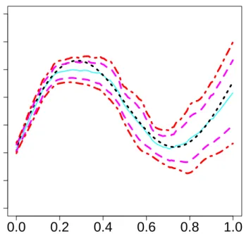
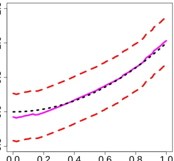
Figure 1 shows the theoretical 0.9 quantile curve, 0.9 quantile estimate with corresponding 95% uniform confidence band from the asymptotic theory and the confidence band from the bootstrap. The real 0.9 quantile curve is marked as the black dotted line. We then compute the classic local quantile estimate lh(x) (cyan solid) with its corresponding 95% uniform confidence
band (magenta dashed) based on asymptotic theory according to H¨ardle and Song (2010). The 95% confidence band from the bootstrap is displayed as
0.0
0.2
0.4
0.6
0.8
1.0
-1.0
0.0
1
.0
2.0
Univariate X
90%
Q
uan
til
e o
f
Y
Figure 1: The real 0.9 quantile curve, 0.9 quantile estimate with correspond-ing 95% uniform confidence band from asymptotic theory and confidence band from bootstrapping.
red dashed-dot lines. At first sight, the quantile smoother, together with two corresponding bands, all capture the heteroscedastic structure quite well, and the width of the bootstrap confidence band is similar to the one based on asymptotic theory in H¨ardle and Song (2010).
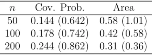
To compare the small sample performance and convergence rate of both methods, Table 1 presents the simulated coverage probabilities together with the calculated area of the 95% confidence band of the quantile smoother, for three sample sizes, n= 50,100 and 200. 500 simulation runs are carried out and for each simulation, 500 bootstrap samples are generated. From Table 1 we observe that, for the asymptotic method, coverage probabilities improve with increasing sample size and the bootstrap method (shown in brackets) obtains a significantly larger coverage probability than the asymptotic one, though still smaller than the nominal coverage, which results from the fact that quantile regression usually needs a larger sample size than mean regres-sion and n here is quite moderate. It is also observed that the size of the bands decrease with increasing sample size. Overall, the bootstrap method displays a better convergence rate, while not sacrificing much on the width of the bands.
n Cov. Prob. Area 50 0.144 (0.642) 0.58 (1.01) 100 0.178 (0.742) 0.42 (0.58) 200 0.244 (0.862) 0.31 (0.36)
Table 1: Simulated coverage probabilities & areas of nominal asymptotic (bootstrap) 95% confidence bands with 500 repetition.
We now extend x to the multivariate case and use a different quantile function to verify our method. Choosex= (u, v)>∈Rd, v ∈
R, and generate
the data {(Ui, Vi, Yi)}ni=1, n= 1000 with:
y= 2u+v2+ε−1.2816, (23) where u and v are uniformly distributed random variables in [0,2] and [0,1] respectively. ε has a standard normal distribution. The theoretical 0. 9-quantile curve is ˜l(x) = 2u+v2. Since the choice of a
n is uncertain here,
we test different choices of an for different n by simulation. To this end, we
modify the theoretical model as follows:
y= 2u+v2 +ε−Φ−1(p)
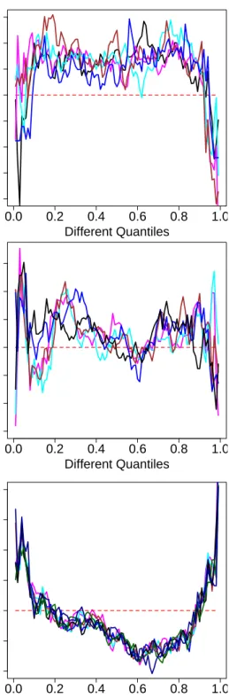
such that the real β is always equal to 2 no matter if p is 0.01 or 0.99. The result is displayed in Figure 2 forn= 1000,n= 8000,n = 261148 (number of observations for the data set used in the following application part). Different lines correspond to differentan, i.e. n1/3/8,n1/3/4,n1/3/2,n1/3,n1/3·2,n1/3·4
and n1/3·8. At first, it seems that the choice of a
n doesn’t matter too much.
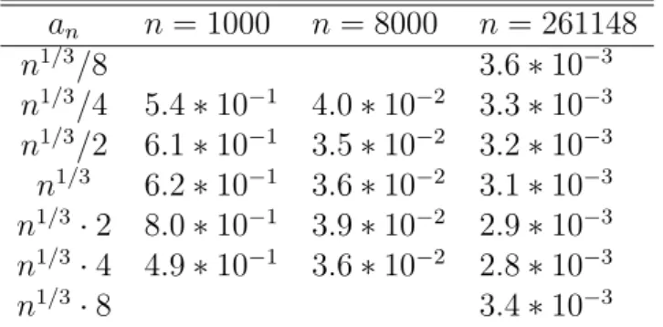
To further investigate this, we calculate the SSE (P99
1 {βˆ(i/100)−β}) where ˆ
β(i/100) denotes the estimate corresponding to the i/100 quantile. Results are displayed in Table 2. Obviously an has much less effect than n on SSE.
Considering computational cost, which increases with an, and estimation
performance, empirically we suggest an = n1/3. Certainly this issue is far
from settled and needs further investigations.
Thus for the specific model (23), we have an = 10, βˆ = 1.997, h = 0.2
and g = 0.7. In Figure 3 the theoretical 0.9 quantile curve with respect tov, and the 0.9 quantile estimate with corresponding uniform confidence band are displayed. The real 0.9 quantile curve is marked as the black dotted line. We then compute the quantile smoother lh(x) (magenta solid). The 95%
bootstrap uniform confidence band is displayed as red dashed lines and cover the true quantile curve quite well.
an n = 1000 n = 8000 n = 261148 n1/3/8 3.6∗10−3 n1/3/4 5.4∗10−1 4.0∗10−2 3.3∗10−3 n1/3/2 6.1∗10−1 3.5∗10−2 3.2∗10−3 n1/3 6.2∗10−1 3.6∗10−2 3.1∗10−3 n1/3·2 8.0∗10−1 3.9∗10−2 2.9∗10−3 n1/3·4 4.9∗10−1 3.6∗10−2 2.8∗10−3 n1/3·8 3.4∗10−3
Table 2: SSE of ˆβ with respect to an for different numbers of observations.
5
A labour market application
Our intuition of the effect of education on income is summarised by Day and Newburger (2002)’s basic claim: “At most ages, more education equates with higher earnings, and the payoff is most notable at the highest educational levels”, which is actually from the point of view of mean regression. However, whether this difference is significant or not is still questionable, especially for different ends of the (conditionally) income distribution. To this end, a careful investigation of quantile regression is necessary. Since different education levels may reflect different productivity, which is unobservable and may also results from different ages, abilities etc, to study the labour market differential effect with respect to different education levels, a semiparametric partial linear quantile model is preferred, which can retain the flexibility of the nonparametric models for the age and other unobservable factors and ease the interpretation of the education factor.
We use the administrative data from the German National Pension Office (Deutsche Rentenversicherung Bund) for the following group: West Germany part, males aged 25−59, born between 1939 and 1942 who began receiving a pension in 2004 or 2005, with at least 30 yearly uncensored observations, and thus in total, n = 128429 observations are available. We have the fol-lowing three education categories: “low education”, “apprenticeship” and “university” for the variable u (assign them the numerical values 1, 2 and 3 respectively); the variable v is the age of the employee. “Low education” means without post-secondary education in Germany. “Apprenticeship” are part of Germany’s dual education system. Depending on the profession, they may work for three to four days a week in the company and then spend one or two days at a vocational school (Berufsschule). “University” in Germany also includes the technical colleges (applied universities). Since the level and
structure of wages differs substantially between East and West Germany, we concentrate on West Germany only here (which we usually refer to simply as Germany). Our data have several advantages over the most often used Ger-man Socio-Economics Panel (GSOEP) data to analyze wages in GerGer-many. Firstly, it is available for a much longer period, as opposed to from 1984 only for the GSOEP data. Secondly, more importantly, it has a much larger sample size. Thirdly, wages are likely to be measured much more precisely. Fourthly, we observe a complete earnings history from the individual’s first job until his retirement, therefore this is a true panel, not a pseudo-panel. There are also several drawbacks. For example, some very wealthy individ-uals are not registered in the German pension system, e.g. if the monthly income is more than some threshold (which may vary for different years due to the inflation effect), the individual has the right not to be included in the public pension system, and thus not recorded. Besides this, it is also right-censored at the highest level of earnings that are subject to social security contributions, so the censored observations in the data are only for those who actually decided to stay within the public system. Because of the com-bination of truncation and censoring, this paper focuses on the uncensored data only, and we should not draw inferences from the very high quantile. Recently, similar data is also used to investigate the German wage structure as in Dustmann et al. (2009).
Following from Becker (1994)’s human capital mode, a log transformation is performed first on the hourly real wages (unit: EUR, in year 2000 prices). Figure 4 displays the boxplots for the “low education”, “apprenticeship” and “university” groups corresponding to different ages. In the data all ages (25 ∼ 59) are reported as integers and are categorised in one-year groups. We rescaled them to the interval [0,1] by dividing by 40, with a corresponding bandwidth of 0.059 for the nonparametric quantile smoothers. This is equiv-alent to setting a bandwidth 2 in the original age data. This makes sense, because to detect whether a differential effect for different education levels exists, we compare the corresponding uniform confidence bands, i.e. differ-ences indicate that the differential effect may exist for different education levels in the German labour market for that specific labour group.
Following an application of the partial linear model in Section 3, Fig-ure 5 displays ˆβ with respect to different quantiles for 6, 13, 25 partitions, respectively. At first, the ˆβ curve is quite surprising, since it is not, as in mean regression, a positive constant, but rather varies a lot, e.g. ˆβ(0.20) = 0.026, βˆ(0.50) = 0.057 and ˆβ(0.80) = 0.061. Furthermore, it is robust to different numbers of partitions. It seems that the differences between the “low education” and “university” groups are different for different tails of the wage distribution. To judge whether these differences are significant, we
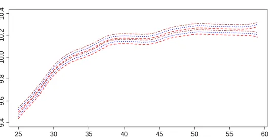
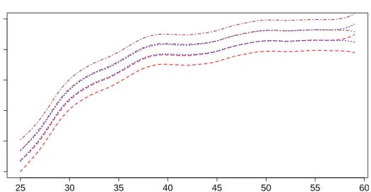
use the uniform confidence band techniques discussed in Section 2 which are displayed in Figure 6 - 8 corresponding to the 0.20, 0.50 and 0.80 quantiles respectively.
The 95% uniform confidence bands from bootstrapping for the “low edu-cation” group are marked as red dashed lines, while the ones for “apprentice-ship” and “university” are displayed as blue dotted and brown dashed-dot lines, respectively. For the 0.20 quantile in Figure 6, the bands for “univer-sity”, “apprenticeship” and “low education” do not differ significantly from one another although they become progressively lower, which indicates that high education does not equate to higher earnings significantly for the lower tails of wages, while increasing age seems the main driving force. For the 0.50 quantile in Figure 7, the bands for “university” and “low education” differ significantly from one another although not from “apprenticeship”’s. However, for the 0.80-quantiles in Figure 8, all the bands differ significantly (except on the right boundary because of the nonparametric method’s bound-ary effect) resulting from the relatively large ˆβ(0.80) = 0.061, which indicates that high education is significantly associated with higher earnings for the uppers tails of wages.
If we investigate the explanations for the differences in different tails of the income distribution, maybe the most prominent reason is the rapid development of technology, which has been extensively studied. The point is technology does not simply increase the demand for upper-end labour realtive to that of lower-end labour, but instead asymmetrically affects the bottom and the top of the wage distribution, resulting in its strong asymmetry.
Conclusions from the point of view of quantile regression are consistent with the (grouped) mean regression’s, but in a careful way, i.e. we pro-vide formal statistical tools to judge these uniformly. Partial linear quantile regression techniques, together with confidence bands, as developed in this paper, display very interesting findings compared with classic (mean) meth-ods. Motivated by several key observations like the average income for female employees increase more than men’s during the past few decades, partially because a better social welfare system means women can be more and more selective; and the “hollowing out” effect of employment, i.e. job growth in U.S., U.K. and continental Europe has increasingly been concentrated in the tails of the skill distribution over the last two decades, with disproportionate employment gains in high-wage, high-education occupations and low-wage, low-education occupations, further applications, for example to different gen-ders, labour union status, nationalities and inequality analysis amongst other things will definitely bring more contributions to the differential analysis of the labour market.
0.0 0.2 0.4 0.6 0.8 1.0 1.80 1.90 2.00 2.10 Different Quantiles B e ta E s ti ma tes 0.0 0.2 0.4 0.6 0.8 1.0 1.94 1.98 2.02 2.06 Different Quantiles B e ta E s ti ma tes 0.0 0.2 0.4 0.6 0.8 1.0 1.990 2.000 2.010 2.020 Different Quantiles B e ta E s ti ma tes
Figure 2: ˆβ with respect to different quantiles for different numbers of ob-servations, i.e. n = 1000,n = 8000,n= 261148.
0.0
0.2
0.4
0.6
0.8
1.0
-0.5
0.0
0
.5
1.0
1
.5
V
N
onparame
tr
ic
P
ar
t
Figure 3: Nonparametric part smoothing, real 0.9 quantile curve with re-spect to v, 0.9 quantile smoother with corresponding 95% bootstrap uniform confidence band. 25 42 59 7.5 8 .0 8.5 9 .0 9.5 10.5 Ages
Log Real Earnings
Figure 4: Boxplots for “low education”, “apprenticeship” & “university” groups corresponding to different ages.
0.0 0.2 0.4 0.6 0.8 1.0 0.00 0.02 0.04 0.06 0.08 0.10 Different Quantiles Beta Estimates
Figure 5: ˆβ corresponding to different quantiles with 6, 13, 25 partitions.
25 30 35 40 45 50 55 60 9.4 9 .6 9.8 10.0 10.2 10.4 Ages
Log Real Earnings
Figure 6: 95% uniform confidence bands for 0.05-quantile smoothers with 3 different education levels
25 30 35 40 45 50 55 60 9.6 9 .8 10.0 10.2 10.4 10.6 Ages
Log Real Earnings
Figure 7: 95% uniform confidence bands for 0.50-quantile smoothers with 3 different education levels
25 30 35 40 45 50 55 60 10.0 10.2 10.4 10.6 10.8 Ages
Log Real Earnings
Figure 8: 95% uniform confidence bands for 0.99-quantile smoothers with 3 different education levels
6
Appendix
Proof of Theorem 2.1 We start by proving equation (7). Write first
ˆ
F−1(Ui|Xi) = F−1(Ui|Xi) + ∆i. Fix any i such that |F−1(Ui|Xi)| ≤ Snδn,
which, by equation (1), implies that |Ui−p|< Snδn. Lemma 2.1 gives:
max
i |
ˆ
F(Sn2δn|Xi)−F(Sn2δn|Xi)|=Op(δn). (24)
Together with F(±Sn2δn|Xi) = p± O(Sn2δn) again by equation (1), we have
ˆ F(±S2 nδn|Xi) =p± Op(Sn2δn) and thus ˆ F(−Sn2δn|Xi) =p− Op(Sn2δn) < p−Snδn< Ui < p+Snδn < p+Op(Sn2δn) = ˆF(Sn2δn|Xi).
Since ˆF(·|Xi) is monotone non-decreasing,|Fˆ−1(Ui|Xi)| ≤Sn2δn, which means,
by Sn2 =Sn,
|Fˆ−1(Ui|Xi)| ≤Snδn. (25)
Apply now Lemma 2.1 again to equation (25), and obtain:
Snδ3/2 ≥ |Fˆi{Fˆ−1(Ui|Xi)} −F{Fˆ−1(Ui|Xi)|Xi}| = |Ui−F{F−1(Ui|Xi) + ∆i|Xi}| = |F{F−1(Ui|Xi)|Xi} −F{F−1(Ui|Xi) + ∆i|Xi}| ≥ f0(Xi)|∆i| (26) Hence |∆i|< Snδ 3/2
n , and we summarise it as:
max
i:|F−1(U
i|Xi)−F−1(p)|<Snδn
|F−1(Ui|Xi)−Fb−1(Ui|Xi)|=Op{Snδn3/2}.
Beside the above approach, there is an alternative way. Note that
|Fˆ−1(U
i|Xi)| ≤ |F−1(Ui|Xi)|+|∆i| ≤Snδn+|∆i|. Similar to inequality (26),
by applying Lemma 2.1, we have Snδn(|∆i|+Snδn)1/2 ≥f0(Xi)|∆i|. Solving
this inequality w.r.t. |∆i| gives:
|∆i|<{Snδ2n+ (Snδn2 + 4Snδn3)1/2}/2 = Op(Snδn3/2),
which leads to the same conclusion. To show equation (11), define
Z1j def = Yj∗−lg(Xj) +lg(Xj)−lg(Xi) Z2j def = Yj#−l(Xj) +l(Xj)−l(Xi).
Thus qhi[{Yj∗−lg(Xj) +lg(Xj)−lg(Xi)})nj=1] and qhi[{Y
#
j −l(Xj) +l(Xj)− l(Xi)}nj=1] can be seen aslh(Xi) for data sets{(Xi, Z1i)}ni=1 and{(Xi, Z2i)}ni=1 respectively. Similar to H¨ardle and Song (2010), they can be treated as a zero (w.r.t. θ, θ ∈ I where I is a possibly infinite, or possibly degenerate, interval in R) of the functions
e Gn(θ, Xi) def = n−1 n X j=1 Kh(Xi−Xj)ψ(Z1j −θ), (27) e e Gn(θ, Xi) def = n−1 n X j=1 Kh(Xi−Xj)ψ(Z2j −θ). (28)
From (7) and (8), we have
max i [{Y ∗ j −lg(Xj) +lg(Xj)−lg(Xi)})nj=1]−[{Y # j −l(Xj) +l(Xj)−l(Xi)}nj=1] = Op{Snδn3/2}+Op(δn) =Op(δn) (29) Thus sup θ∈I max i |Gen(θ, Xi)− e e Gn(θ, Xi)| ≤ Op(δn) max|n−1 X Kh|=Op(δn)
To show the difference of the two quantile smoothers, we shall reduce the strong convergence of qhi[{Yj∗ −lg(Xj) +lg(Xj)−lg(Xi)})nj=1]−qhi[{Yj#− l(Xj) +l(Xj)−l(Xi)}nj=1], for any i, to an application of the strong conver-gence ofGe(θ, Xi) toGeen(θ, Xi), uniformly in θ, for any i. Under assumptions
(A7) and (A8), in a similar spirit of H¨ardle and Song (2010), we get max i |l ∗ h(Xi)−lg(Xi)−l # h(Xi)−l(Xi)|=Op(δn).
To show the supremum of the bootstrap approximation error, without loss of generality, based on assumption (A1), we reorder the original observations
{Xi, Yi}ni=1, such that X1 6X2 6. . . ,6Xn. First decompose:
sup x∈J∗ |l∗h(x)−lg(x)−l#h(x)−l(x)|= maxi |l ∗ h(Xi)−lg(Xi)−l#h(Xi)−l(Xi)| + max i x∈[Xsup i,Xi+1] |lh∗(x)−lg(x)−lh#(x)−l(x)|.(30)
From assumption (A1) we knowl0(·)≤λ1 and maxi(Xi+1−Xi) = Op(Sn/n).
By the mean value theorem, we conclude that the second term of (30) is of a lower order than the first term. Together with equation (11) we have
sup x∈J∗ |l∗h(x)−lg(x)−lh#(x)−l(x)| = O{max i |l ∗ h(Xi)−lg(Xi)−l#h(Xi)−l(Xi)|}=Op(δn),
which means that the supremum of the approximation error over all x is of the same order of the maximum over the discrete observed Xi.
Proof of Theorem 2.2. The proof of (14) uses methods related to those in
the proof of Theorem 3 of H¨ardle and Marron (1991), so only the main steps are explicitly given. The first step is a bias-variance decomposition,
E h n ˆ bh,g(x)−bh(x) o2 |X1, ...Xn i =Vn+B2n (31) where Vn = Var h ˆ bh,g(x)|X1, ...Xn i , B2 n = E h ˆb h,g(x)−bh(x)|X1, ...Xn i .
Following the uniform Bahadur representation techniques for quantile re-gression as in Theorem 3.2 of Kong et al. (2008), we have the following linear approximation for the quantile smoother as a local polynomial smoother cor-responding to a specific loss function:
l#h(x)−l(x) =Ln+Op(Ln), where Ln= n−1P Kh(x−Xi)ψ{Yi−l(x)} f{l(x)|x}fX(x)
for ψ(u) = p1{u∈(0,∞)} −(1−p)1{u∈(−∞,0)} = p−1{u∈(−∞,0)}, l(x−t)−l(x) = l0(x)(−t) +l00(x)t2+O(t2), {l(x−t)−l(x)}0 = l00(x)(−t) +l000(x)t2+O(t2), f(x−t) = f(x) +f0(x)(−t) +f00(x)(t2) +O(t2), f0(x−t) = f0(x) +f00(x)(−t) +f000(x)t2+O(t2), Z Kh(t)tdt = 0, Z Kh(t)t2dt = h2dK, Z Kh(t)O(t2)dt = O(h2). Then we have Bn=Bn1+O(Bn1), where Bn1 = R Kg(x−t)Uh(t)dt− Uh(x) fX(x)f{l(x)|x} for Uh(x) = Z Kh(x−s)ψ{l(s)−l(x)}f(s)ds = Z Kh(t)ψ{l(x−t)−l(x)}f(x−t)dt.
By differentiation, a Taylor expansion and properties of the kernel K (see assumption (A2)), Uh0(x) = Z Kh(t)[ψ0{l(x−t)−l(x)} 0 f(x−t) +ψ{l(x−t)−l(x)}f0(x−t)]dt.
Collecting terms, we get
Uh0(x) = Z Kh(t){ψ0l00(x)fX0 (x)t 2 +ψ0l000fX(x)t2 +af000(x)t2+O(t2)}dt = Z Kh(t) C0t2+o(t2) dt =h2dK·C0+O(h2),
where a is a constant with |a| < 1 and C0 = ψ0l00(x)fX0 (x) +ψ0l000fX(x) + af000(x).
Hence, by another substitution and Taylor expansion, for the first term in the numerator of Bn1, we have
Bn2 =g2h2(dK)2·C0+O(g2h2). Thus, along almost all sample sequences,
B2
n=C1g4h4+O(g4h4) (32) for C1 = (dK)4C02/[fX2(x)f2{l(x)|x}].
For the variance term, calculation in a similar spirit shows that
Vn =Vn1+O(Vn1), where Vn1 = R Kg2(x−t)Wh(t)dt− { R Kg(x−t)Uh(t)dt}2fX(x)f{l(x)|x} fX(x)f{l(x)|x} for Wh(x) = Z Kh2(x−s)ψ{l(s)−l(x)}2f(s)ds = Z Kh2(t)ψ{l(x−t)−l(x)}2f(x−t)dt.
Hence, by Taylor expansion, collecting items and similar calculation, we have
Vn=n−1h4g−5C2+O(n−1h4g−5) (33) for a constant C2. This, together with (31) and (32) completes the proof of Theorem 2.2.
Proof of Theorem 3.1. In case the function l is known, the estimate ˆβI is:
ˆ βI = argmin β n X i=1 ψ{Yi−l(Vi)−Ui>β}.
Since l is unknown, in each of these small intervals Ini, l(Vi) could be
regarded as a constant α = l(mni) for some i whose corresponding interval Ini covers Vi. From assumption (A1), we know that |l(Vi)−αi| ≤λ1bn <∞.
( ˆαi,βˆi) = argmin α, β
X
ψ(Yi−α−Ui>β),
|{Yi −l(Vi)−Ui>β} −(Yi−α−Ui>β)| ≤ λ1bn <∞ indicates that we could
treat ˆβi as ˆβI inside each partition. If we use di to denote the number
of observations inside partition Ini (based on the i.i.d. assumption as in
assumption (A1), on average di =n/an). For each of the ˆβi inside interval Ini, various parametric quantile regression literature, e.g. the convex function
rule in Pollard (1991) and Knight (2001) yields
p
di( ˆβi−β)
L
→N{0, p(1−p)D0−i 1(p)Ci0D0−i 1(p)} (34) with the matricesCi0 =di−1Pid=1i Ui>UiandDi0(p) =di−1Pdi=1i f{l(Vi)|Vi}Ui>Ui.
To get ˆβ, our second step is to take the weighted mean of ˆβ1, . . . ,βˆan as:
ˆ β = arg min β an X i=1 di( ˆβi−β)2 = an X i=1 diβˆi/n
Please note that under this construction, ˆβ1, . . . ,βˆan are independent but
not identical. Thus we intend to use the Lindeberg condition for the central limit theorem. To this end, we use s2
n to denote Var(
Pan
i=1diβˆi/n), and we
need to further check whether the following “Lindeberg condition” holds:
lim an→∞ 1 s2 n an X i=1 Z (|diβˆi/n−β|>εsn) ( ˆβi−β)2dF = 0, for all ε >0. (35) Since Var( an X i=1 diβˆi/n) = an X i p(1−p) nh n/di di X j=1 f{l(Vj)|v}Uj>Uj i−1 × di X i=1 Ui>Ui h n/di di X j=1 f{l(Vj)|v}Uj>Uj i−1o ≈ p(1−p)h n X j=1 f{l(Vj)|v}Uj>Uj i−1 × n X i=1 Ui>Ui hXn j=1 f{l(Vj)|v}Uj>Uj i−1 def = 1 np(1−p)D −1 n CnDn−1,
where Dn= n1 Pn j=1f{l(Vj)|Vi}Uj>Uj and Cn= 1n Pn i=1U > i Ui, together with
the normality of ˆβi as in (34) and properties of the tail of the normal
distri-bution, e.g. Exe. 14.3−14.4 of Borak et al. (2010), (35) follows.
Thus as n, an → ∞ (although at a lower rate than n), together with C = plimn→∞Cn, D= plimn→∞Dn, we have
√
n( ˆβ−β)→L N{0, p(1−p)D−1CD−1}. (36)
References
Becker, G. (1994). Human Capital: A Theoretical and Empirical Analysis with Special Reference to Education, 3rd edition. The University of Chicago Press.
Belloni, A. and Chernozhukov, V. (2009). l1-penalized quantile regression in high-dimensional sparse models. CEMMAP Working Paper, 10/09. Borak, S., H¨ardle, W., and Lopez, B. (2010). Statistics of Financial Markets
Exercises and Solutions. Springer-Verlag, Heidelberg.
Buchinsky, M. (1995). Quantile regression, box-cox transformation model, and the u.s. wage structure, 1963-1987. Journal of Econometrics, 65:109– 154.
Chernozhukov, V., Lee, S., and Rosen, A. M. (2009). Intersection bounds: estimation and inference. CEMMAP Working Paper, 19/09.
Day, J. C. and Newburger, E. C. (2002). The big payoff: Educational attain-ment and synthetic estimates of work-life earnings. special studies. current population reports. Statistical report p23-210, U.S. Department of Com-merce Economics and Statistics Administration, U.S. CENSUS BUREAU. Denby, L. (1986). Smooth regression functions. Statistical report 26, AT&T
Bell Laboratories.
Dustmann, C., Ludsteck, J., and Sch¨onberg, U. (2009). Revisitng the german wage structure. Quartely Journal of Economics, forthcoming.
Fisher, R. A. and Tippett, L. H. C. (1928). Limiting forms of the fre-quency distribution of the largest or smallest member of a sample. Proc. Cambridge Philos. Soc., 24:180–190.
Franke, J. and Mwita, P. (2003). Nonparametric estimates for conditional quantiles of time series. Report in Wirtschaftsmathematik 87, University of Kaiserslautern.
Green, P. J. and Yandell, B. S. (1985). Semi-parametric generalized linear models. In Proceedings 2nd International GLIM Conference, volume 32 of Lecture Notes in Statistics 32, pages 44–55, New York. Springer.
Hahn, J. (1995). Bootstrapping quantile regression estimators. Econometric Theory, 11(1):105–121.
Hall, P. (1991). On convergence rates of suprema. Probab. Th. Rel. Fields, 89:447–455.
H¨ardle, W., Janssen, P., and Serfling, R. (1988). Strong uniform consistency rates for estimators of conditional functionals. Ann. Statist., 16:1428–1429. H¨ardle, W. and Luckhaus, S. (1984). Uniform consistency of a class of
re-gression function estimators. Ann. Statist., 12:612–623.
H¨ardle, W. and Marron, J. (1991). Bootstrap simultaneous error bars for nonparametric regression. Ann. Statist., 19:778–796.
H¨ardle, W. and Song, S. (2010). Confidence bands in quantile regression. Econometric Theory, 26:1–22.
Horowitz, J. L. (1998). Bootstrap methods for median regression models. Econometrica, 66(6):1327–1351.
Knight, K. (2001). Comparing conditional quantile estimators: first and second order considerations. Unpublished manuscript.
Koenker, R. and Bassett, G. W. (1978). Regression quantiles. Econometrica, 46:33–50.
Koenker, R. and Hallock, K. F. (2001). Quantile regression. Journal of Econometric Perspectives, 15(4):143–156.
Kong, E., Linton, O., and Xia, Y. (2008). Uniform Bahadur representation for local polynomial estimates of M-regression and its application to the additive model. Econometric Theory, accepted.
Kuan, C., Yeh, J., and Hsu, Y. (2009). Assessing value at risk with care, the conditional autoregressive expectile models. Journal of Econometrics, 150:261–270.
Liang, H. and Li, R. (2009). Variable selection for partially linear models with measurement errors. J. Amer. Statist. Assoc., forthcoming.
Newey, W. and Powell, J. (1987). Asymmetric least squares estimation and testing. Econometrica, 55:816C847.
Pollard, D. (1991). Asymptotics for least absolute deviation estimators. Econometric Theory, 7:186–199.
Robinson, P. M. (1988). Semiparametric econometrics: A survey. Journal of Applied Econometrics, 3:35–51.
Speckman, P. E. (1988). Regression analysis for partially linear models. 50:413–436.
Yu, K. and Jones, M. C. (1998). Local linear quantile regression. J. Amer. Statist. Assoc., 93:228–237.
SFB 649 Discussion Paper Series 2010
For a complete list of Discussion Papers published by the SFB 649, please visit http://sfb649.wiwi.hu-berlin.de.
001 "Volatility Investing with Variance Swaps" by Wolfgang Karl Härdle and Elena Silyakova, January 2010.
002 "Partial Linear Quantile Regression and Bootstrap Confidence Bands" by Wolfgang Karl Härdle, Ya’acov Ritov and Song Song, January 2010.