Modeling High Frequency Data Using Hawkes Processes
with Power-Law Kernels
∗
Changyong Zhang
Department of Finance and Banking, Faculty of Business, Curtin University Sarawak, Malaysia
Abstract
Those empirical properties exhibited by high frequency financial data, such as time-varying intensities and self-exciting features, make it a challenge to model appropriately the dynamics associated with, for instance, order arrival. To capture the microscopic structures pertaining to limit order books, this paper focuses on modeling high frequency financial data using Hawkes processes. Specifically, the model with power-law kernels is compared with the counterpart with exponential kernels, on the goodness of fit to the empirical data, based on a number of proposed quantities for statistical tests. Based on one-trading-day data of one representative stock, it is shown that Hawkes processes with power-law kernels are able to reproduce the intensity of jumps in the price processes more accurately, which suggests that they could serve as a realistic model for high frequency data on the level of microstructure.
Keywords: High frequency data, Hawkes processes, intensity kernel
1
Introduction
The prices of financial assets are driven by the interaction of buy and sell orders. Today more and more equity exchanges have been organized as order-driven markets, where the orders are aggregated in a limit order book, which is available to market participants. At a given time the limit order book states the quantities of the underlying asset that are posted at each price level. The limit order book can be seen as a complex data generating process and modern information technology allows traders in equity markets to process information, including order submissions and cancelations, at high frequency and high speed. The traders/firms who utilize the new technology for intraday trading for their own accounts are generally called high frequency traders (HFTs), who are now major players in equity markets (Boehmer et al.,2013;Brogaard et al.,2013;Hagstr¨omer and Norden,2013;Hendershott and Riordan,2011;Hendershott et al.,
2011; Jovanovic and Menkveld,2011;Kirilenko et al.,2011;Menkveld,2011).
In an order-driven market, the price dynamics of a financial asset is the result of the dynamics of the limit order book. HFTs try to model the dynamics, using more or less sophistical
∗An extended version of this paper can be found athttp://dx.doi.org/10.13140/2.1.2398.2085
Volume 80, 2016, Pages 762–771
ICCS 2016. The International Conference on Computational Science
762 Selection and peer-review under responsibility of the Scientific Programme Committee of ICCS 2016 c
techniques, conditioning on information about the history and the current state of the order book, to make predictions concerning its short-term behavior as well as the direction of price moves. Fundamentally, models of order book dynamics provide insights into the interplay between order flow and price evolution (Bouchaud et al., 2002; Doyne Farmer et al., 2004;
Foucault et al.,2005). Among the growing literature on modeling the dynamics of order books, are equilibrium models (Foucault,1999;Parlour,1998), dynamic expected utility maximization models (Parlour,1998;Rosu,2009), and models based on queuing system or self-exciting point processes (A¨ıt-Sahalia et al., 2011; Bauwens and Hautsch,2009;Cont et al.,2010).
Due to the complexity involved in the underlying dynamics, most of the aforementioned models have difficulties in describing reasonably precisely the order book dynamics and hence the price dynamics of the financial asset. It is a challenge to formulate statistically realistic and quantitatively feasible models for the dynamics of limit order books. In particular, on the one hand, statistical features of order book dynamics, which are revealed by empirical studies concerning properties of limit order books, are usually unrealistic to be represented in a single model (Bouchaud et al.,2002;Doyne Farmer et al.,2004;Hollifield et al.,2004). On the other hand, a significant number of existing stochastic models assume steady-state distributions, which are not necessarily verified by real high frequency data (Bouchaud et al., 2009; Cont et al., 2010;Luckock,2003;Maslov and Mills, 2001; Smith et al.,2003).
Specifically, from a statistical perspective, modeling high-frequency data is challenging due to the presence of strong autocorrelations in the order flow, time-varying intensities of events, and cross-correlations between the arrival rates of different types of orders and potentially between different markets. These features can not be captured by standard Poisson point processes. Meanwhile, Hawkes processes possess flexible statistical properties allowing to in-corporate autocorrelations and self-exciting features. Unlike time-series models such as ACD-GARCH, they remain analytically tractable. Likelihood functions, conditional distributions, moments, Laplace transforms, and characteristic functions may be computed analytically or by solving ODEs. Due to their mathematical tractability and ability to account for clustering effects, since their introduction (Hawkes, 1971; Vere-Jones, 1970), they have been widely ap-plied in, for instance, seismology (Ogata,1999;Zhuang et al.,2002), shot noises (Br´emaud and Massouli´e,2002), biology (Coleman and Gastwirth,1969;Reynaud-Bouret and Schbath,2010), criminology (Mohler et al.,2011). In finance, Hawkes processes are used in estimating VaR and valuing credit derivatives (Chavez-Demoulin et al., 2005;Embrechts et al.,2011; Errais et al.,
2010;Giesecke et al.,2011), and in modeling market event data, microstructure noise, and clus-ters of extremes (Abergel and Jedidi,2011;Bacry et al.,2013;Bacry and Muzy,2014;Bauwens and Hautsch,2009;Bormetti et al.,2013; Bowsher,2007;Chavez-Demoulin and McGill,2012;
Cont,2011;Filimonov and Sornette,2012;Filimonov et al., 2014; Zheng et al.,2014).
Hawkes processes with distinguishable kernels exhibit different behaviors. In the literature, more studies have been on Hawkes processes with exponential kernels (Hawkes, 1971; Ogata,
1981;Ozaki,1979). This paper focuses on modeling high frequency data using Hawkes processes, in particular, with power-law kernels, and studying the difference between power-law kernels and exponential kernels. In Section2, models based on Hawkes processes are briefly discussed. Empirical results on high frequency data are then reported in Section 3. Section 4 outlines directions for possible future work.
2
Hawkes-Based Models
Consider an asset traded in a single market. Assume that each jump time the price moves by 1 tick only. Then it can be modeled using a Hawkes process (Bacry et al.,2013). LetP0 be the
price at time 0. The model for the price at timet is
Pt=P0+Nt1−Nt2, (1)
where Nt1 is the number of upward jumps in the price and Nt2 is that of downward jumps
between 0 and t. The jump processesNt1 andNt2 are assumed to have intensities λ1t and λ2t,
respectively, with λit=μi+ 2 j=1 t 0 φ ij t−sdNsj, i= 1,2, (2)
whereμis a deterministic base intensity and the decay kernelφrepresents the influence of past events on the current value of the intensity process, withφij
s ≥0,∀s≥0, i, j= 1, . . . ,2. In particular, if φij s =αije−β ijs in (2), then λit=μi+ 2 j=1 t 0 αij eβij(t−s)dNsj, i= 1,2, (3) whereαij >0,βij>0, and αij βij <1,i, j= 1, . . . ,2. Similarly, ifφijs = α ij (s+γij)βij, then λi t=μi+ 2 j=1 t 0 αij (t−s+γij)βijdNsj, i= 1,2, (4) whereαij >0,βij>1, andγij >0,i, j= 1,2.
The model defined in (3) results in a bivariate Hawkes process with exponential kernels and that in (4) results in a bivariate Hawkes process with power law kernels. The model based on the latter is the focus of this paper and in Section3it is demonstrated to capture the dynamics of a limit order book more accurately than the counterpart based on the former.
3
Empirical Study
The two models (3) and (4) are implemented in MATLAB. For efficiency in estimating the parameters, it is first assumed that μ1 =μ2, α11 = α22, α12 = α21, β11 = β22, β12 = β21, and γ11 = γ12 = γ21 = γ22, respectively in both models. Since the focus is on comparison between the two types of kernels, the underlying price process does not affect the result and the study is based on the best bid of ERICB (Ericsson Telephone Company) on the trading day of September 7th, 2012. For comparison, the same price process (1) needs to be assumed, where P ={Pt}t≥0 denote the best bid, N1={Nt1}t≥0 the number of upward jumps with intensity
λ1, andN2={Nt2}t≥0the number of downward jumps with intensityλ2.
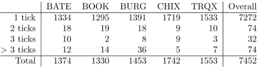
As a starting point, to verify the assumption that the price moves by at most one tick at each instance, the jump sizes on five exchanges are examined. As shown in Table 1, overall more than 97% (72727452 = 0.9758) of all jumps in the best bid was 1 tick only on September 7th, 2012. On the two exchanges BOOK (Nasdaq OMX Stockholm) and CHIX (Chi-X), the corresponding numbers are 97% (12951330 = 0.9737) and 98% (17191742 = 0.9868), respectively. Hence, it is reasonable to first make the assumption that the best bid moves by 1 tick for each jump.
To compare the goodness of fit of the two models with the real data, a number of measures are introduced first.
Let N1 denote the number of upward jumps, N2 the number downward jumps, Pmax the maximum price observed, andPminthe minimum price observed, of the price evolution pathPt
BATE BOOK BURG CHIX TRQX Overall 1 tick 1334 1295 1391 1719 1533 7272 2 ticks 18 19 18 9 10 74 3 ticks 10 2 8 9 3 32 >3 ticks 12 14 36 5 7 74 Total 1374 1330 1453 1742 1553 7452
Table 1: Jumps of Best Bid of ERICB on Five Exchanges on 07/09/2012
of the real data within a certain time interval, denoted as (0, T] after being shifted. Accordingly, ˆ
N1, ˆN2, ˆPmax, and ˆPminare the counterparts of a sample path ˆPtgenerated from a model with
the estimated values of the parameters (ˆμ,α,ˆ β,ˆ γˆ). ˆNtis the estimated value of E[Nt].
First, let ˆ S(L) = 1 L L l=1 ˆ Pmax(l)−Pˆmin(l) Pmax−Pmin ,
where L is the number of simulated paths, ˆPmax(l) and ˆPmin(l) are the highest and lowest prices observed from the lth simulated sample path, respectively. ˆS thus measures the price fluctuation of the simulated paths relative to that of the real data.
Fori= 1,2, denote ˆ Ri(L) = 1 L L l=1 |Nˆi(l)−Ni| Ni .
Here ˆRi indicates how far ˆNi diverges fromNi and so how well the underlying model fits the data in terms of number of jumps.
Next, define ˆ Mi(L) = 1 L L l=1 M m=1 |Nˆi (tm−1,tm](l)−N i (tm−1,tm]| Ni , i= 1,2 and ˆ V(L) = 1 L L l=1 T 0 | ˆ Pt(l)−Pt|dt,
where {tm}m=0,1,...,M is an even partition of the time interval (0, T] with t0 = 0 andtM =T,
Ni
(tm−1,tm]is the number of jumps within (tm−1, tm] from the real data, and ˆN
i
(tm−1,tm](l) is that
of thelth simulated sample path. Here it is takentm−tm−1= 1s,m= 1, . . . , M. ˆMi, i= 1,2
hence measure the overall discrepancy between the simulated paths and the evolution path from the real data in both intensity and clustering of jumps. From a different perspective, ˆV measures the total divergence of the simulated paths from the original evolution path.
To test the estimated results, a one-sample Student’st-test is run for each ˆNi,i= 1,2 from
each model. For each test, let ¯xbe the sample mean,s the sample standard deviation, andn the number of sample paths generated. Then to verify the null hypothesis that the population mean associated with a model is equal to the corresponding value μ0 of the real data, the
t-statistic is obtained as
t= x¯−sμ0
√
n
To test whether there is a discrepancy between the estimated results from the two models, i.e., the null hypothesis that the two population means of the two models are equal, a Welch’s t-test is conducted for each of ˆNi, ˆMi, ˆS, and ˆV, i= 1,2. Since the same number of sample
pathsnare generated for both models, for each test, the t-statistic is then t=x¯√1−x¯2
s21+s22
√
n
,
where ¯xi,s2i,i= 1,2 are the sample mean and sample variance estimated from the two models,
respectively.
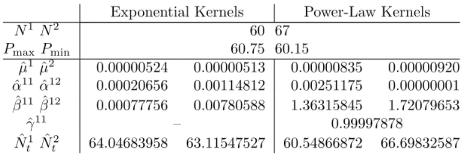
To compare the two models, 1000 sample paths are generated from each of them for the best bid of ERICB on the exchange CHIX in a two-hour time period (10:00-12:00) on September 6th, 2012. The estimated results, the Student’st-tests for ˆNi,i= 1,2, and the Welch’st-tests
for the measures are provided in Tables2,3,4, respectively.
Exponential Kernels Power-Law Kernels
N1N2 60 67 PmaxPmin 60.75 60.15 ˆ μ1μˆ2 0.00000524 0.00000513 0.00000835 0.00000920 ˆ α11αˆ12 0.00020656 0.00114812 0.00251175 0.00000001 ˆ β11βˆ12 0.00077756 0.00780588 1.36315845 1.72079653 ˆ γ11 – 0.99997878 ˆ Nt1Nˆt2 64.04683958 63.11547527 60.54866872 66.69832587
Table 2: MLE of Best Bid of ERICB on CHIX from 10:00 to 12:00 on 06/09/2012
Exponential Kernels Power-Law Kernels t-statistic p-value t-statistic p-value ˆ
N1 11.957 <0.0001 0.692 0.4890 ˆ
N2 -10.603 <0.0001 -2.927 0.0036
Table 3: Student’st-Tests for Numbers of Jumps of Best Bid of ERICB on CHIX from 10:00 to 12:00 on 06/09/2012
As shown in Table4, thep-values of both ˆN1 and ˆN2 are less than 0.01%, which indicates that there is a significant difference between the numbers of both upward and downward jumps estimated from the two models. This is further backed up by the results presented in Table3. For the model with power-law kernels, thep-values of both ˆN1 and ˆN2 are greater than 0.1%, which means with a significance level 0.001, the null hypothesis that the mean numbers of both upward and downward jumps of the simulated paths equal the counterparts of the real data cannot be rejected. It is hence statistically verified that the intensity of jumps of the simulated path is in accordance with that of the evolution path of the data. Clearly, this is not the case for the model with exponential kernels, bothp-values of which are far less than 0.01%, which tells that the null hypothesis should be rejected under the same significance level.
In Table 4, the p-values of both ˆS and ˆV are less than 0.01%, which implies that the differences between the corresponding population means of the two models are significant.
Exponential Kernels Power-Law Kernels Welch’st Test
Mean Variance Mean Variance t-statistic p-value
ˆ N1 64.36000000 132.96136136 60.17000000 60.42752753 9.528 <0.0001 ˆ N2 63.10700000 134.79434535 66.23000000 69.22432432 -6.914 <0.0001 ˆ S 1.58341667 0.27408658 1.48450000 0.26104858 4.276 <0.0001 ˆ M1 2.05726667 0.03649425 1.98723333 0.01697399 9.578 <0.0001 ˆ M2 1.92702985 0.03005025 1.97122388 0.01564826 -6.538 <0.0001 ˆ V 0.86936802 0.26599960 0.65889510 0.12928692 10.586 <0.0001 Table 4: Welch’st-Tests for Best Bid of ERICB on CHIX from 10:00 to 12:00 on 06/09/2012
The sample means of both measures of the model with power-law kernels are less than the counterparts of the model with exponential kernels. This indicates that the model with power-law kernels is more stable in capturing the price movement and that on average the simulated paths diverge from the original price evolution path less than the one with exponential kernels. The only measure that does not differentiate the two models is ˆM. The model with power-law kernels outperforms the one with exponential kernels in ˆM1and vice versa in ˆM2. A plausible explanation of this is that the two models result in different numbers of jumps of the simulated paths. Larger number of jumps potentially leads to larger value of ˆM, provided that jumps do not occur intensively.
From the statistical studies, it can thus be inferred that overall the model with power-law kernels fits the real data better than the one with exponential kernels.
4
Conclusion
Hawkes processes with power-law kernels are studied and compared with Hawkes processes with exponential kernels for modeling high frequency data. It is verified by numerical results that the former fits real data better than the latter, which suggests that a Hawkes-based model with power-law kernels be an appropriate choice for high frequency data.
The results obtained in this paper are based on the data of one stock on one trading day. An immediate extension is then, for robustness study, to generalize the results on data of one stock on multiple trading days and data of multiple stocks on one trading day. It is also interesting to look into the computational efficiencies of different algorithms to search for the maximum likelihood estimator.
The study focuses on models for one stock with jumps of 1 tick at most on one exchange. There are several possible extensions, including the cases that one stock in different time in-tervals, different stocks in the same time interval, and one stock on different markets. For example, it has been observed that the intensities of jumps in different time intervals follow different patterns, which indicates that it is worth considering dividing a whole trading day into sub-intervals and modeling them separately.
In reality, the price may move by more than 1 tick, as shown in Table1. Suppose the price of an asset moves up to dticks for a jump, then the price can be described as a multivariate Hawkes model, Pt=P0+ d i=1 i·Nti,1− d i=1 i·Nti,2,
where P0 is the price at time 0,Ni,1 is the number of upward jumps withi ticks, andNi,2 is that of downward jumps withiticks between 0 andt,i= 1, . . . , d. The intensities ofNi,1 and
Ni,2 areλi,1 andλi,2, respectively, λi,kt =μi,k+ d j=1 t 0 φ ij,k1 t−s dNsj,1+ d j=1 t 0 φ ij,k2 t−s dNsj,2, k= 1,2.
It has been widely recognized that the price evolution of a stock is heavily affected by large orders. Another direction is then to take into consideration the factor of market impactAlmgren and Chriss(2000);Bertsimas and Lo(1998).
Acknowledgements
This research has been supported by a grant from Riksbankens Jubileumsfond (P10 - 0113:1). The author greatly acknowledges Kaj Nystr¨om for motivating the study and gratefully appre-ciate NasdaqOMX in Stockholm for providing the high frequency financial data.
References
Fr´ed´eric Abergel and Aymen Jedidi. A mathematical approach to order book modelling. In Fr´ed´eric Abergel, Bikas K. Chakrabarti, Anirban Chakraborti, and Manipushpak Mitra, edi-tors,Econophysics of Order-driven Markets, New Economic Windows, pages 93–107. Springer Milan, 2011.
Yacine A¨ıt-Sahalia, Per A. Mykland, and Lan Zhang. Ultra high frequency volatility estimation with dependent microstructure noise. Journal of Econometrics, 160:160–175, 2011.
Robert Almgren and Neil Chriss. Optimal execution of portfolio transactions. Journal of Risk, 3(2):5–39, 2000.
E. Bacry, S. Delattre, M. Hoffmann, and J. F. Muzy. Modelling microstructure noise with mutually exciting point processes. Quant. Finance, 13(1):65–77, 2013.
Emmanuel Bacry and Jean-Fran¸cois Muzy. Hawkes model for price and trades high-frequency dynamics. Quantitative Finance, 14(7):1147–1166, 2014.
Luc Bauwens and Nikolaus Hautsch. Modelling financial high frequency data using point pro-cesses. In Thomas Mikosch, Jens-Peter Kreiß, Richard A. Davis, and Torben Gustav Ander-sen, editors,Handbook of Financial Time Series, pages 953–979. Springer Berlin Heidelberg, 2009.
Dimitris Bertsimas and Andrew W. Lo. Optimal control of execution costs.Journal of Financial Markets, 1(1):1–50, 1998.
Ekkehart Boehmer, Kingsley Y. L. Fong, and Juan Wu. International evidence on algorithmic trading. AFA 2013 san diego meetings paper, 2013.
Giacomo Bormetti, Lucio Maria Calcagnile, Michele Treccani, Fulvio Corsi, Stefano Marmi, and Fabrizio Lillo. Modelling systemic price cojumps with hawkes factor models. http://ssrn.com/abstract=2209139, 2013.
Jean-Philippe Bouchaud, Marc M´ezard, and Marc Potters. Statistical properties of stock order books: empirical results and models. Quantitative Finance, 2(4):251–256, 2002.
Jean-Philippe Bouchaud, J. Doyne Farmer, and Fabrizio Lillo. How markets slowly digest changes in supply and demand. In Thorsten Hens and Klaus Reiner Schenk-Hoppe, edi-tors,Handbook of financial markets: dynamics and evolution, pages 57–160. Elsevier, North-Holland, 2009.
Clive G. Bowsher. Modelling security market events in continuous time: Intensity based, multivariate point process models. Journal of Econometrics, 141(2):876–912, 2007.
Pierre Br´emaud and Laurent Massouli´e. Power spectra of general shot noises and hawkes point processes with a random excitation. Advances in Applied Probability, 34(1):205–222, 2002. Jonathan Brogaard, Terrence Hendershott, and Ryan Riordan. High frequency trading and
price discovery. Working paper, 2013.
V. Chavez-Demoulin and J.A. McGill. High-frequency financial data modeling using hawkes processes. Journal of Banking & Finance, 36(12):3415 – 3426, 2012.
V. Chavez-Demoulin, A. C. Davison, and A. J. McNeil. Estimating value-at-risk: a point process approach. Quantitative Finance, 5(2):227–234, 2005.
R. Coleman and J. L. Gastwirth. Some models for interaction of renewal processes related to neuron firing. J. Appl. Probability, 6:38–58, 1969.
Rama Cont. Statistical modeling of high-frequency financial data. IEEE Signal Processing Magazine, 28(5):16–25, 2011.
Rama Cont, Sasha Stoikov, and Rishi Talreja. A stochastic model for order book dynamics.
Operations Research, 58(3):549–563, 2010.
J. Doyne Farmer, L´aszl´o Gillemot, Fabrizio Lillo, Szabolcs Mike, and Anindya Sen. What really causes large price changes? Quantitative Finance, 4(4):383–397, 2004.
Paul Embrechts, Thomas Liniger, and Lu Lin. Multivariate Hawkes processes: an application to financial data. Journal of Applied Probability, 48:367–378, 2011.
Eymen Errais, Kay Giesecke, and Lisa R. Goldberg. Affine point processes and portfolio credit risk. SIAM J. Financial Math., 1(1):642–665, 2010.
Vladimir Filimonov and Didier Sornette. Quantifying reflexivity in financial markets: Toward a prediction of flash crashes. Phys. Rev. E, 85:056108, May 2012.
Vladimir Filimonov, David Bicchetti, Nicolas Maystre, and Didier Sornette. Quantification of the high level of endogeneity and of structural regime shifts in commodity markets. Journal of International Money and Finance, 42(0):174 – 192, 2014.
Thierry Foucault. Order flow composition and trading costs in a dynamic limit order market.
Journal of Financial Markets, 2(2):99 – 134, 1999.
Thierry Foucault, Ohad Kadan, and Eugene Kandel. Limit order book as a market for liquidity.
Kay Giesecke, Lisa R. Goldberg, and Xiaowei Ding. A top-down approach to multiname credit.
Operations Research, 59(2):283–300, 2011.
Bj¨orn Hagstr¨omer and Lars L. Norden. The diversity of high-frequency traders. Working paper, 2013.
Alan G. Hawkes. Spectra of some self-exciting and mutually exciting point processes.
Biometrika, 58(1):83–90, 1971.
Terrence Hendershott and Ryan Riordan. Algorithmic trading and information. Working paper, 2011.
Terrence Hendershott, Charles M. Jones, and Albert J. Menkveld. Does algorithmic trading improve liquidity? Journal of Finance, 66(1):1–33, 2011.
Burton Hollifield, Robert A. Miller, and Patrik Sand˚as. Empirical analysis of limit order markets. The Review of Economic Studies, 71(4):1027–1063, 2004.
Boyan Jovanovic and Albert J. Menkveld. Middlemen in limit-order markets. Western finance association (WFA), 2011.
Andrei A. Kirilenko, Albert S. Kyle, Mehrdad Samadi, and Tugkan Tuzun. The flash crash: The impact of high frequency trading on an electronic market. Working paper, 2011. Hugh Luckock. A steady-state model of the continuous double auction. Quantitative Finance,
3(5):385–404, 2003.
Sergei Maslov and Mark Mills. Price fluctuations from the order book perspective - Empirical facts and a simple model. Physica A, 299:234–246, 2001.
Albert J. Menkveld. High frequency trading and the new-market makers. Tinbergen Institute Discussion Papers 11-076/2/DSF21, 2011.
G. O. Mohler, M. B. Short, P. J. Brantingham, F. P. Schoenberg, and G. E. Tita. Self-Exciting Point Process Modeling of Crime. Journal of the American Statistical Association, 106(493): 100–108, 2011.
Yosihiko Ogata. On Lewis’ Simulation Method for Point Processes. IEEE Transactions on Information Theory, 27(1):23–30, 1981.
Yosihiko Ogata. Seismicity analysis through point-process modeling: A review. Pure and Applied Geophysics, 155(2-4):471–507, 1999.
T. Ozaki. Maximum likelihood estimation of Hawkes’ self-exciting point processes. Ann. Inst. Statist. Math., 31(1):145–155, 1979.
Christine A Parlour. Price dynamics in limit order markets. Review of Financial Studies, 11 (4):789–816, 1998.
Patricia Reynaud-Bouret and Sophie Schbath. Adaptive estimation for Hawkes processes; ap-plication to genome analysis. The Annals of Statistics, 38:2781–2822, 2010.
Ioanid Rosu. A dynamic model of the limit order book. Review of Financial Studies, 22(11): 4601–4641, 2009.
Eric Smith, Doyne J. Farmer, Laszlo Gillemot, and Supriya Krishnamurthy. Statistical theory of the continuous double auction. Quantitative Finance, 3:481–514, 2003.
D. Vere-Jones. Stochastic models for earthquake occurrence. Journal of the Royal Statistical Society. Series B(Methodological), 32(1):1–62, 1970.
Ban Zheng, Fran¸cois Roueff, and Fr´ed´eric Abergel. Modelling bid and ask prices using con-strained hawkes processes: Ergodicity and scaling limit. SIAM Journal on Financial Math-ematics, 5(1):99–136, 2014.
Jiancang Zhuang, Yosihiko Ogata, and David Vere-Jones. Stochastic declustering of space-time earthquake occurrences. Journal of the American Statistical Association, 97(458):369–380, 2002.