Turun kauppakorkeakoulu • Turku School of Economics
ABSTRACT
Bachelor’s thesis x Master’s thesis Licentiate’s thesis Doctoral dissertationSubject Economics Date 1.6.2020
Author(s) Joonas Pajukoski Student number 508083
Number of pages 84 Title Predicting credit rating change using machine learning and natural
lan-guage processing
Supervisor(s) Ph.D. Janne Tukiainen
Abstract
Corporate credit ratings provide standardized third-party information for market participants. They offer many benefits for issuers, intermediaries and investors and generally increase trust and efficiency in the market. Credit ratings are provided by credit rating agencies. In addition to quan-titative information of companies (e.g. financial statements), the qualitative information in com-pany-related textual documents is known to be a determinant in the credit rating process. How-ever, the way in which the credit rating agencies interpret this data is not public information.
The purpose of this thesis is to develop a supervised machine learning model that predicts credit rating changes as a binary classification problem, based on form 10-k annual reports of public U.S. companies. Before using in the classification task, the form 10-k reports are prepro-cessed using natural language processing methods. More generally, this thesis aims to answer, to what extent a change in a company’s credit rating can be predicted based on the form 10-k reports, and whether the use of topic modeling can improve the results. A total of five different machine learning algorithms are used for the binary classification of this thesis and their performances are compared. These algorithms are support vector machine, logistic regression, decision tree, ran-dom forest and naïve Bayes classifier. Topic modeling is implemented using latent semantic anal-ysis.
The studies of Hajek et al. (2016) and Chen et al. (2017) are the main sources of inspiration for this thesis. The methods used in this thesis are for the most part similar as in these studies. This thesis adds value to the findings of these studies by finding out how credit rating prediction methods in Hajek et al. (2016), binary classification methods in Chen et al. (2017) and utilization of form 10-k annual reports (used in both Hajek et al. (2016) and Chen et al. (2017) can be com-bined as a binary credit rating classifier.
The results of the study show that credit rating change can be predicted using 10-k data, but the predictions are not very accurate. The best classification results were obtained using a support vector machine, with an accuracy of 69.4% and an AUC of 0.6744. No significant improvement on classification performance was obtained using topic modeling.
Key words Machine learning, natural language processing, credit rating prediction Further
in-formation -
Turun kauppakorkeakoulu • Turku School of Economics
TIIVISTELMÄ
Kandidaatintutkielma x Pro gradu -tutkielma
Lisensiaatintutkielma Väitöskirja
Oppiaine Taloustiede Päivämäärä 1.6.2020
Tekijä(t) Joonas Pajukoski Matrikkelinumero 508083
Sivumäärä 84
Otsikko Predicting credit rating change using machine learning and natural lan-guage processing
Ohjaaja(t) VTT Janne Tukiainen
Tiivistelmä
Yritysten luottoluokitukset antavat standardoitua kolmannen osapuolen tietoa markkinaosapuolille. Ne tarjoavat monia etuja liikkeellelaskijoille, välittäjille ja sijoittajille ja lisäävät yleistä luottamusta ja tehokkuutta markkinoilla. Luottoluokituksia myöntävät luottoluokituslaitokset. Kvantitatiivisten yritystä koskevien tietojen (esim. Tilinpäätöstietojen) lisäksi yrityksen julkaiseman tekstimuotoisen datan sisältävien laadullisten tietojen tiedetään vaikuttavan luottoluokitusprosessiin. Tapa, jolla luottoluokituslaitokset tulkitsevat tätä tietoa, ei kuitenkaan ole julkisesti tiedossa.
Tämän tutkielman tarkoituksena on kehittää ohjattu koneoppimismalli, joka ennustaa luottoluokitusmuutoksia binäärisenä luokitteluongelmana Yhdysvalloissa toimivien pörssiyhtiöiden 10-k -muotoisten vuosikertomuksien perusteella. 10-k vuosikertomukset esikäsitellään luonnollisen kielen käsittelyn menetelmillä, ennen kuin niitä käytetään luokittelutehtävässä. Yleisemmin tämän tutkielman tavoitteena on selvittää, missä määrin yrityksen luottoluokituksen muutosta voidaan ennustaa 10-k vuosikertomuksen perusteella ja voidaanko aihemallinnuksen avulla parantaa tuloksia. Tutkielmassa käytetään binääriseen luokitteluun yhteensä viittä erilaista koneoppimisalgoritmia ja verrataan niiden suorituskykyjä. Nämä algoritmit ovat tukivektorikone, logistinen regressio, päätöspuu, satunnainen metsä ja naïve Bayes-luokitin. Aihemallinnus toteutetaan latentin semanttisen analyysin avulla.
Hajek ym. (2016) ja Chen ym. (2017) tutkimukset ovat toimineet pääasiallisena inspiraation lähteenä tälle tutkielmalle. Tässä tutkielmassa käytetyt metodit ovat pitkälti samoja kuin näissä tutkimuksissa. Tämä tutkielma tuo lisäarvoa näiden tutkimusten tuloksiin selvittämällä, kuinka Hajek ym. (2016) käyttämiä luottoluokituksen ennustusmetodeja, Chen ym. (2017) käyttämiä binäärisen luokittelun metodeja ja 10-k vuosikertomusten hyödyntämistä (käytetty sekä Hajek ym. (2016) että Chen ym. (2017)) voidaan yhdistää binääriseksi luottoluokitusennustimeksi.
Tutkielman tulokset osoittavat, että luottoluokituksen muutosta voidaan ennustaa käyttämällä 10-k vuosikertomuksia, mutta ennusteet eivät ole kovin tarkkoja. Paras luokittelutulos saatiin tukivektorikoneella, tarkkuudella 69,4% ja AUC-arvolla 0,6744. Aihemallinnuksella ei saavutettu merkittävää parannusta luokittelutuloksiin.
Avainsanat Koneoppiminen, luonnollisen kielen käsittely, luottoluokitusmuutoksen ennustaminen
PREDICTING CREDIT RATING CHANGE USING
MACHINE LEARNING AND NATURAL
LANGUAGE PROCESSING
Master’s Thesis in economics Author(s): Joonas Pajukoski Supervisor(s): Ph.D. Janne Tukiainen 1.6.2020 TurkuThe originality of this thesis has been checked in accordance with the University of Turku quality assurance system using the Turnitin OriginalityCheck service.
TABLE OF CONTENTS
1 INTRODUCTION ... 9
2 THEORETICAL BACKGROUND ... 12
2.1 Corporate credit rating ... 12
2.2 Machine learning ... 14
2.2.1 The relationship between ML and statistics ... 15
2.2.2 Types of learning ... 16
2.2.3 Train-test -split ... 17
2.2.4 Overfitting and validation ... 18
2.2.5 Bias-variance (complexity) trade-off ... 20
2.2.6 Prediction accuracy and model interpretability trade-off ... 21
2.2.7 Handling imbalanced classes ... 21
2.2.8 Evaluation metrics ... 23
2.3 Natural language processing ... 25
2.3.1 Text preprocessing techniques ... 26
2.3.2 Bag-of-words (BOW) and vectorization ... 28
2.3.3 Topic modeling ... 30
3 RELATED LITERATURE ... 32
4 DATA AND METHODS USED IN THE STUDY ... 34
4.1 Form 10-k annual reports ... 34
4.2 Data preparation ... 34
4.3 Data limitations ... 35
4.4 Data preprocessing and feature extraction ... 36
4.5 Train-test split and validation ... 37
4.6 Latent semantic analysis (LSA) ... 37
4.7 Machine learning algorithms ... 39
4.7.2 Logistic regression ... 46
4.7.3 Decision trees ... 48
4.7.4 Random forest ... 51
4.7.5 Naïve Bayes classifier ... 53
5 RESULTS ... 55
5.1 Bag-of-words ... 55
5.1.1 Support vector machine ... 55
5.1.2 Logistic regression ... 57
5.1.3 Decision tree ... 58
5.1.4 Random forest ... 60
5.1.5 Naïve Bayes classifier ... 62
5.2 Topic modeling ... 64
5.2.1 Support vector machine ... 64
5.2.2 Logistic regression ... 65
5.2.3 Decision tree ... 67
5.2.4 Random forest ... 69
5.2.5 Naïve Bayes classifier ... 71
5.3 Summary of the results ... 73
6 CONCLUSIONS AND RECOMMENDATIONS FOR FURTHER RESEARCH ... 75
LIST OF FIGURES
Figure 1. Standard & Poor’s credit rating classes (Adapted from Spglobal.com). ... 13
Figure 2. An example of overfitting (Marsland 2014). ... 19
Figure 3. Sampling techniques (Vluymans 2019). ... 22
Figure 4. Confusion matrix (Adapted from Alpaydin 2014). ... 23
Figure 5. ROC-curve (James et al. 2013)... 25
Figure 6. A simple TD matrix (Jurafsky & Martin 2018). ... 28
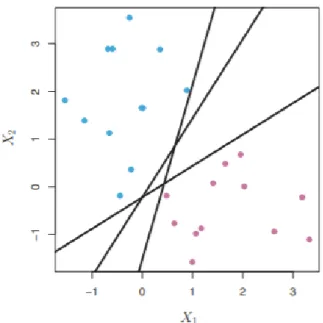
Figure 7. Separating hyperplanes (James et al. 2013). ... 40
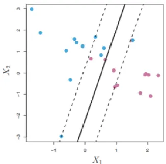
Figure 8. The maximal margin hyperplane (James et al. 2013). ... 41
Figure 9. A soft margin classifier (James et al. 2013). ... 42
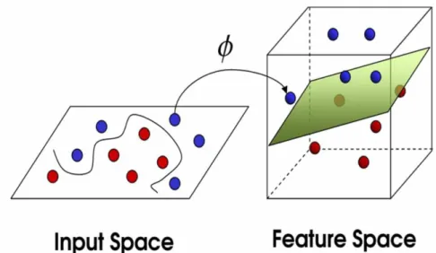
Figure 10. Mapping input vectors into feature space using kernel (Kaundal et al. 2006)…. ... 43
Figure 11. Binary classification performed with polynomial and radial kernels (James et al. 2013). ... 45
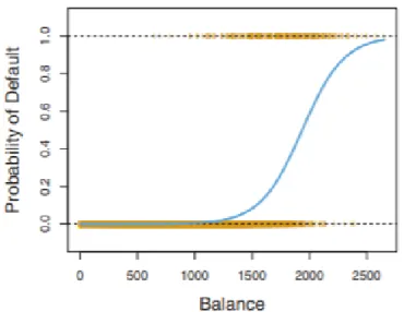
Figure 12. An example of a sigmoidal function (James et al. 2013). ... 47
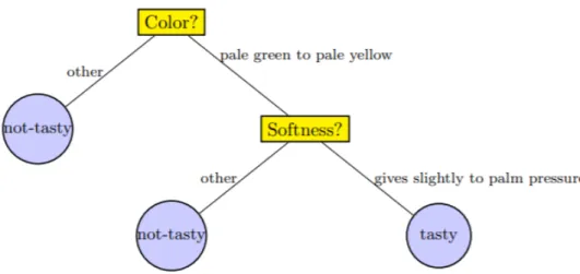
Figure 13. Binary classification tree model (Shai & Shai 2014). ... 48
LIST OF TABLES
Table 1. Used datasets ... 36
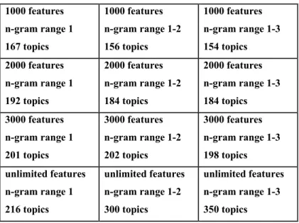
Table 2. Optimal number of topics for each dataset. ... 38
Table 3. SVM classification results (BOW). ... 56
Table 4. SVM confusion matrices (BOW). ... 56
Table 5. Logistic regression classification results (BOW)... 57
Table 6. Logistic regression confusion matrices (BOW). ... 58
Table 7. Optimal hyperparameter values for decision tree (BOW). ... 59
Table 8. Decision tree classification results (BOW). ... 59
Table 9. Decision tree confusion matrices (BOW). ... 60
Table 10. Optimal hyperparameter values for random forest (BOW). ... 61
Table 11. Random forest classification results (BOW). ... 61
Table 12. Random forest confusion matrices (BOW). ... 62
Table 13. MNB classification results (BOW). ... 63
Table 14. MNB confusion matrices (BOW). ... 63
Table 15. SVM classification results (topic modeling). ... 64
Table 16. SVM confusion matrices (topic modeling). ... 65
Table 17. Logistic regression classification results (topic modeling). ... 66
Table 18. Logistic regression confusion matrices (topic modeling). ... 67
Table 19. Optimal hyperparameters for decision tree (topic modeling). ... 68
Table 20. Decision tree classification results (topic modeling). ... 68
Table 21. Decision tree confusion matrices (topic modeling). ... 69
Table 22. Optimal hyperparameters for random forest (topic modeling). ... 70
Table 23. Random forest classification results (topic modeling). ... 70
Table 24. Random forest confusion matrices (topic modeling). ... 71
Table 25. MNB classification results (topic modeling). ... 72
LIST OF ABBREVIATIONS
ML Machine learning
NLP Natural language processing
BOW Bag-of-words
SMOTE Synthetic Minority Over-sampling Technique
ROC Receiver operator characteristics
AUC Area under the curve
POS Part-of-speech
TD Term-document
TF-IDF Term Frequency – Inverse Document Frequency
LSA Latent semantic analysis
SVD Singular value decomposition
SVM Support vector machine
KNN K-nearest neighbors
ANN Artificial neural network
SEC U.S. Securities and Exchange Commission IBDR Integrated binary discriminant rule
1
INTRODUCTION
Over the last few years, there has been a growing interest in implementing machine learn-ing (ML) methods for financial forecastlearn-ing purposes. Numerous studies have been con-ducted on the prediction capabilities of ML methods, for example, in stock price move-ments and corporate bankruptcies. Another popular prediction task concerning the finan-cial sector is corporate credit ratings. Credit rating represents the creditworthiness1 of a
company. Thus, it provides crucial information to the company’s stakeholders. The ability to predict credit ratings makes it possible to detect the problems of the company of interest at an early stage.
Credit ratings are issued by credit rating agencies. These agencies openly report on their websites the factors on the basis of which they issue the ratings. However, the re-ported factors include only those that can be measured quantitatively. Among the variety of information, financial ratios available in financial statements are the most important
factors determining a company’s credit rating. Therefore, credit ratings can be predicted quite accurately based on them alone. Nevertheless, it is known that qualitative factors are also considered in the process. The exact methods used by credit rating agencies to utilize qualitative information from textual data published by companies are not publicly known.
Hajek et al. (2016) developed a methodology to address this issue. They extracted topical content from form 10-k annual reports and examined how it could be utilized to predict credit ratings, using some popular ML algorithms. Therefore, the task at hand was solved as a multi-class prediction problem. The obtained predictions were combined with the more traditional approach, where financial ratios are used as predictor variables. The study suggested that in the 10-k reports, there might be some hidden information useful for credit rating prediction. Chen et al. (2017), in turn, used topical content of 10-k reports to predict bank failures. They implemented the prediction as a binary classification task to try to determine whether the bank will default in the next period or not.
Utilizing ideas from both of these studies, the aim of this thesis is to develop a meth-odology to predict credit rating changes as a binary classification problem. First, using 10-k reports and credit ratings from corresponding years (from Standard & Poor’s), the
1 Creditworthiness means the company’s ability to meet its payable commitments (Hajek et al., 2016).
ability to predict a change in credit rating is examined using a bag-of-words (BOW) ap-proach. The BOW is a widely used natural language processing (NLP) method, in which individual words and combinations of words in text documents are used as predictor var-iables. After the examination of the BOW approach, it is examined whether the use of topic modeling improves the prediction performance or not. Both Hajek et al. (2016) and Chen et al. (2017) state that the BOW approach tends to overfit the data, yielding therefore a limited prediction performance. Thus, one could assume that the prediction results can be improved utilizing the topic modeling methods used by Hajek et al. (2016) and Chen et al. (2017).
A total of five widely used ML algorithms are trained for the prediction task, and their performances are compared. This way, a predictive model, designed to add value to another model outside of this work, is construct. Ultimately, the constructed model is able to output the probability that the credit rating of the company under consideration will either decrease or increase. The prediction model constructed in this study can be applied to any 10-k report that has not been used to train the model. In this way, the possible credit rating change of a company of interest can be assessed on the basis of a 10-k report.
Thus, the constructed model provides an estimate of the development of the company’s
financial condition in the near future.
At a more general level, this thesis answers the following research questions:
1. To what extent can a company’s credit rating change be predicted utilizing the
textual data of the previous period’s form 10-k annual report? 2. Can the prediction performance be improved using topic modeling?
The theoretical framework of this study provides first a quick overview of corporate credit ratings; what they are and why they are important. After that, a more detailed re-view of ML is given in section 2.2. It includes a theoretical definition of ML in general, a breakdown of the similarities and differences between ML and statistics, an overview of the more practical features of ML and some metrics to evaluate the learning process. In addition to ML, another important theoretical entity regarding this thesis is natural language processing (NLP). A few essential NLP methods are described in section 2.3. After these a bit more technical sections, some previous studies related to this thesis are reviewed in section 3.
Section 4 gives a description of the data and methods that were utilized in this thesis. The section explains what kind of data was used, and how it was processed before use. A total of five different ML algorithms are used in this thesis to predict corporate credit ratings. Their basic characteristics are described in section 4.7.
The results, obtained using the theoretical framework and methods described in sec-tions 2 and 4, are presented in section 5. The last section concludes the findings of the study and proposes recommendations for future research on this topic.
2
THEORETICAL BACKGROUND
2.1 Corporate credit rating
The purpose of credit rating is to provide standardized, forward-looking third-party infor-mation for market participants. They comprehensively increase trust and thus efficiency in the market. Credit ratings are used by issuers, intermediaries and investors. For issuers, for example companies, credit ratings allow the company to provide reliable information about its own creditworthiness and financial strength to the market. This is an effective way to increase operational transparency and reliability to current investors, and also to widen the pool of potential future investors, which may reduce the cost of funding.
Gen-erally, for a company’s stakeholders, credit rating indicates the financial condition of the company. Credit ratings play an important role in, for example, the decisions concerning
a company’s capital structure. Credit ratings also allow companies to obtain more favor-able terms of financing. Similarly, the financiers of a company can monitor a company's solvency through loan covenants in which a credit rating acts as a trigger. In addition to companies, credit ratings are assigned also for other issuers of specific types debt, for example nations and local governments. (Spglobal.com, Shin et al. 2012.)
For intermediaries, for example investment banks, credit ratings improve the flow of money from investors to issuers. They can be used to benchmark the relative credit risk of different debt issues; to compare the creditworthiness of companies in an objective fashion. The initial pricing for individual debt issues and the interest rate they pay can be set on the basis of credit ratings. (Spglobal.com.)
Credit ratings provide a third-party opinion of credit quality for investors. Investors, for example pension funds, can use credit ratings to assess credit risk. Credit ratings allow comparing different issuers and debt issues, when making investment decisions and man-aging portfolios. Credit ratings also provide information and metrics to make informed decisions. For investors, this may be supplementing their own credit analysis or estab-lishing thresholds for credit risk and investment guideline. (Spglobal.com.)
Credit ratings vary usually on a scale from Aaa/AAA to D, where Aaa/AAA repre-sents the highest possible creditworthiness and D (default) is assigned in the case of bank-ruptcy. Figure 1. shows the credit rating classes of Standard & Poor’s. The figure demon-strates how the creditworthiness of a company decreases, as the rating class approaches the bottom of the table. Rating classes from AAA to BBB- are often considered as the
investment classes and rating classes from BB+ to D as the non-investment classes, indi-cating how trustworthy a company is as an investment. (Spglobal.com, Hajek et al. 2016.)
Figure 1. Standard & Poor’s credit rating classes (Adapted from Spglobal.com). Credit ratings are issued mainly in two types, short-term and long-term ratings. As the names imply, short-term ratings describe short-term solvency and long-term ratings describe long-term solvency. The credit ratings used in this study are long-term ratings. (Moodys.com.)
Credit ratings are provided by credit rating agencies (eg. Standard & Poor’s, Moody’s
or Fitch), who require a variety of company-related information to complete the rating process. Among the factors affecting the credit rating are, for example, financial state-ments, conference calls, management interviews, corporate annual & quarterly reports etc. As stated in the introduction, quantitatively measurable credit rating determinants are openly reported by credit rating agencies, and they are usually the most important factors, when determining a credit rating. For example, certain values of financial ratios are al-ways associated with certain probabilities of bankruptcy, and thus certain credit ratings. However, a variety of textual data is also considered in the process. This company-related qualitative information is evaluated carefully by the credit rating agencies, for it is as-sumed to contain important information about the financial condition of the company and
Rating AAA AA+ AA AA-A+ investment classes A A-BBB+ BBB+ BBB-BB+ BB BB-B+ B B-CCC+ CCC+ CCC-CC C D non-investment classes cr ed it w o rt h in es s d ec re as es
its future. All in all, the corporate credit rating process is very expertise and time-demand-ing, which for its part explains the growing interest in simulating the process through ML methods. (Hajek et al. 2016.)
2.2 Machine learning
Machine learning is a subfield of artificial intelligence examining intelligent systems that learn. A specific feature of ML, just like of human intelligence, is the ability to learn independently based on experience. As learning enables an artificial agent to become in-dependent of its creator, it can be considered the most fundamental aspect of intelligence. In many occasions, the designer of the agent does not have complete knowledge of the environment where a desirable task is performed. Therefore, the autonomy provided by learning is essential, as it releases the agent from the limited knowledge of the designer and the assumptions built into its original settings. This is one of the relevant differences between traditional programming and ML; an ML model is not dependent on built-in logic. In many implementations, the most successful systems are not constructed by tra-ditional programming, but by a learning process. (Boden 1996.)
Successful actions are what make an agent intelligent (Boden 1996). Thus, an agent cannot be considered intelligent, if it is not able to learn from its mistakes, without being explicitly programmed2. Learning from mistakes decreases both the probability of
corre-sponding occasions and the severity of the consequences caused by these mistakes. This is the essence of ML; the ability of an artificial agent to perform tasks successfully in a changing environment. (Russell & Norvig 2009.)
More practically speaking, ML can be defined as a field, which aims to develop al-gorithms that adapt to exogenous alterations in a desirable way by means of empirical data, experience and training (Kapitanova et al. 2012) or according to Alpaydin (2014), the use of example data or past experience to program a computer to optimize perfor-mance criteria. The basic idea of ML is that the machine gradually learns from input data. As the learning process progresses, the ML model improves its performance and auto-matically learns to make more accurate predictions (if the model is predictive) or to gain better knowledge from data (if the model is descriptive) or both. In an ML model, some
2 Artificial Intelligence pioneer Arthur Samuel defined in 1959 machine learning as a field of study that gives computers the ability to learn without explicit programming (Samuel 1959).
parameters are predefined, and the actual learning process is in practical terms the execu-tion of a computer program and the optimizaexecu-tion of the predefined parameters, using past experience or training data. (Alpaydin 2014.)
ML has a lot in common with optimization. In fact, ML problems are often formed as an optimization problem of a loss function on training data. In this case, a loss function points out the difference between the final predicted values of the chosen ML model and the actual problem instances. Classic optimization theory is however utilized only to train the algorithm; to find the parameters that minimize the loss function on training data, whereas in ML, the main focus is in the performance of the model on unseen test data. This is the crucial difference between optimization and ML. (Le Roux et al. 2012.)
2.2.1 The relationship between ML and statistics
ML and statistics are nowadays somewhat overlapping terms, yet they are not the same thing. However, there would be no ML without statistics, because the models used in ML are based on statistical theories. (Alpaydin, 2014). The principal goal is what practically makes the difference between ML and statistics. Statistics is traditionally used to make inferences from a sample and to detect causal relationships, while ML is heavily focused on recognizing patterns for forecasting purposes and to achieve forecasting results as good as possible. Generally, statistical methods can be utilized in prediction tasks as well, but predictive accuracy is not their strength. Likewise, some ML models may be inter-pretable, but the best predictions are obtained with non-interpretable models. (Bzdok et al. 2018.)
To detect some latent mechanism or to find causal connections in data usually re-quires statistical methods, and these cases tend to be the domain of statistics. However, ML methods enable making accurate predictions, without the need to understand the un-derlying mechanisms. Hence, the model can be learned from data and the explicit struc-ture of the learning process does not need to be known3; the exact way to transform the
known input into the desired output may remain hidden. In ML, the real shape of the function is often thought to be so complex that it cannot be defined beforehand. (Bzdok et al. 2018, Breiman 2001.)
Although their purpose is what makes the major difference, ML and statistics are separated also by other factors. The use of statistical models in ML tasks often causes confusion. For example, why is a simple linear regression sometimes perceived as ML? In ML, a linear regressor can be trained to obtain the same outcome as a statistical regres-sion model, minimizing the squared error between data points, would yield. The answer lies in the way the performance of the model is evaluated. In ML, the performance is
evaluated using a separate subset of data as a “test set4”, whereas the performance of a
statistical model would be determined by the significance and robustness of the model parameters. (Boelaert & Ollion 2018.)
The use of statistical models usually has a strong theoretical basis, whereas the reason why one chooses to use a particular ML method lies primarily in the empirical results. The mechanics of ML algorithms are based on statistical theories, but in practice, algo-rithms that produce the best prediction results are used. Therefore, ML can be said to be very result-oriented. (Boelaert & Ollion 2018.)
The structure and quantity of the data in use has an influence on which one, statistical or ML method, suits best for the concerning case. When the data is considered “wide”
(more input variables than subjects), ML methods are usually effective, whereas statisti-cal methods tend to be more useful, when one is dealing with “long” data (more subjects
than input variables). (Bzdok et al. 2018.)
2.2.2 Types of learning
There are many types of ML algorithms. They have different approaches and are intended to solve different kinds of tasks or problems. They also use different input data and output different results. These learning methods can be roughly divided into two main groups based on their goal and the data available: supervised learning and unsupervised learning. (James et al. 2013.) Their principal characteristics are described in this section.
The purpose in supervised learning is to create a model that predicts the value of a response variable (output) using explanatory variables (input). In ML vocabulary, explan-atory variables are often called features or predictors whereas response variables are called targets or responses. In supervised learning, the required training data is referred
as labeled data. This means that for each predictor in the data, a known response is pro-vided. Supervised learning algorithms can predict the labels of new, unseen observations, based on the information learned from the labeled training data. (James et al. 2013.)
Generalization is what makes supervised ML methods useful. Because of it, the trained algorithm provides reasonable responses for inputs that the algorithm has not en-countered before. This also makes the algorithm capable of dealing with noise (minor discrepancies in the data). (Marsland 2014.)
Supervised ML methods are most commonly used in classification (categorical pre-dicted value) and regression (continuous prepre-dicted value) tasks (James et al. 2013).
In unsupervised learning tasks, there are no labeled training and test data sets. In-stead, the learner identifies similarities between the input variables without any training data. The goal is to find structure and provide a summarized or compressed version of the input data. A typical unsupervised learning task is clustering data into smaller subsets consisting of similar objects. (Marsland 2014.)
The results obtained from unsupervised learning tasks are often utilized in increasing the interpretability of the data for further analysis. Two examples of widely used unsu-pervised learning tasks are dimensionality reduction and grouping. Summaries or com-pressed versions of the data can be obtained with dimensionality reduction techniques. Feature grouping allows labeling the groups based on their content and then the use of supervised learning methods, or the detection of new relationships between features. (James et al. 2013.)
Supervised and unsupervised learning methods are only the most common types of learning and the ones that are relevant to this thesis. Besides them, there are several other types of ML, for example semi-supervised and reinforcement learning. These methods are mixtures of both supervised and unsupervised learning, and are also widely used, but they are not examined in this thesis. (Marsland 2014.)
2.2.3 Train-test -split
In supervised learning, to evaluate the quality of the learning process, the predictions provided by the trained algorithm need to be compared with the known target labels. However, the algorithm needs to generalize to unseen examples, which the algorithm has not encountered in the training data. A separate test set is therefore required to
success-fully evaluate the performance of the algorithm. Practically, this is carried out by detach-ing some predictor-target pairs from the data and thus formdetach-ing a new separate dataset. The predicted outputs, that are based on unseen predictors, can thereafter be compared with the known targets. If the algorithm would be tested on the training data, the results would likely be very (positively) biased. The train-test split unfortunately reduces the amount of training data in use, but one just has to accept it, in order to successfully eval-uate the learning process. (Marsland 2014.)
2.2.4 Overfitting and validation
Overfitting occurs, when an ML model fits the training set “too well”. Besides
learn-ing the actual function, an overfittlearn-ing model also learns the noise and inaccuracies from the data. As a result, the model’s ability to generalize to unseen data decreases and
there-fore the prediction accuracy of an overfitting model is usually poor. An overfitting model has high statistical variance. (Kuhn & Johnson 2013.) Boelaert & Ollion (2018) parallel an overfitting model to a student, who learns perfectly all the exact answers given in class but does not understand the actual reasoning behind them, when preparing for a math exam. This strategy would be successful only in the unlikely case that the exam consists of exactly the same exercises seen already in class. If the teacher changes any numbers in the exercises, the student would fail.
Figure 2. shows two different stages of a simplified learning process. The left-hand side of the figure presents a model that fits the training data well. The training error is small, but not zero, since the curve (learned function) goes near the training data points, but not through them. The right-hand side presents, in turn, a situation, where the model becomes too complex as the learning process continues. The model is now matching the training data perfectly, including the inaccuracies and noise in it, instead of only finding the underlying function. The training error of this kind of model is very close to zero; it is overfitting and not able to generalize to unseen examples. (Marsland 2014.)
Figure 2. An example of overfitting (Marsland 2014).
Along with the training and test sets, a third data set, called the validation set, is required to detect overfitting. As its name suggests, the validation set is used to validate the learning process so far. In other words, validation set is utilized to find out how well the model is generalizing at each moment and to stop the learning process early enough to avoid overfitting. (Marsland 2014.)
If the available data were large enough, it could be divided randomly into k parts and each part could be further divided randomly into two parts. Then, half of each k part could be used for training and half for the model validation. In real world tasks, the data is however rarely sufficient for this. In order to successfully validate the learning process with smaller datasets, a process called cross-validation can be implemented. When using it, the insufficiency of data is compensated by repeatedly splitting the data in a different way. (Alpaydin 2014.)
More specifically, the cross-validation process is commonly carried out using a k-fold cross-validation. In a k-k-fold cross-validation, the training data is divided into k roughly equal-sized subsets (k is usually 5, 10 or 30). After that, the model is fitted and validated k times, using all the subsets alternately for fitting and validation. For example, if a 30-fold cross-validation was performed, the data would first be divided into 30 sets. The model would then be fitted using 29 subsets for learning, and the excluded sub-set would be used as the validation sub-set (to calculate the prediction error). In the next step, the same would be repeated using the second subset as the validation set. This is continued until all 30 subsets have been used as validation sets. This way, the whole data is used for both training and validating the model; to understand how well the model performs the task of learning from some data and predicting some new data. The final performance estimate is obtained from the average of these 30 validations. The validation process is
actually just a way to ensure that the model performs well enough. After the model has been validated, it is trained using all the available training data. An overfitting model typically performs well on the training data but fails when using the test data. (Alpaydin 2014.)
When implementing the k-fold cross-validation technique, in vital importance is to keep the class representations balanced. For example, if class A represents 20 percent of the whole dataset, the subsets drawn from the data as validation sets must also contain approximately 20 percent class A. This is called stratification in ML literature. (Alpaydin 2014, Kuhn & Johnson 2013.)
2.2.5 Bias-variance (complexity) trade-off
As stated above, ML models with high complexity may result in overfitting. But what about a model that is too simple for a given task? According to Marsland (2014), too simple model that is not accurate and does not match the training data well, is said to be biased. For example, a simple linear line fitted to the data in Figure 2. would have a very high bias. This kind of model would have no variance at all, but due to the bad fit to the data, bias would in contrast be very high. A highly biased model does not therefore detect the important connections between the input and output variables (the connections are too complex for the model). A model with a high bias is said to underfit the data (Alpaydin 2014). Overfitting and underfitting are hence the two main reasons, why an ML model may in some cases be unsuccessful.
Generally speaking, bias can be decreased by increasing the complexity of the model, and vice versa. Thus, it is easy to train a very biased, or a very complex model. A well-functioning ML model would however have both low enough bias and low enough com-plexity. This forms a fundamental problem in supervised ML tasks; finding the optimal level of complexity for the model to obtain good results. (James et al. 2013.) The problem is often referred to as the bias-complexity or the bias-variance trade-off.
Hyperparameters are tools that are used to tune the complexity of the model. They are used in almost all modern supervised learning models, and thus they are used also in the empirical part of this thesis. (Probst et al. 2019.)
2.2.6 Prediction accuracy and model interpretability trade-off
The level of complexity is closely linked to the prediction capabilities and interpretability of the model. As noted in chapter 2.2.1., ML algorithms are often unable to detect the exact causal connections between input and output variables. Instead, they tend to be so complex, that the explicit learning process is practically unknown. James et al. (2013) state that there is a trade-off between the prediction accuracy and the interpretability of the model. That is, if the prediction accuracy of a model is preferable in a given task, the interpretability in such a case decreases (e.g. support vector machines (SVM), random forests), and vice versa. Of course, besides “black box” algorithms, there are also simpler ML methods that are easier to interpret (e.g. regression models), but as stated, their pre-diction capabilities tend to be more restricted. Therefore, the right type of algorithm must be chosen based on the intended use.
2.2.7 Handling imbalanced classes
A case, where the (training) data consists of precisely balanced classes (e.g. the targets are either positive or negative, and appear in even proportions in the data), is quite rare. This may possibly cause problems in the learning process. (Marsland 2014.) An efficient predictive model would predict both classes5 accurately, but data imbalance often causes
the model to excessively predict the majority class. This results in a relatively large num-ber of minority class misclassifications. (Vluymans 2019.) Therefore, the results obtained using an imbalanced training data tend to be very skewed (Kuhn & Johnson 2013).
There are many ways to handle the class imbalance. These include for example
tun-ing the model to predict the minority class more sensitively; to lower the model’s minority class predicting threshold. In addition, sampling methods are widely used and effective (e.g. Van Hulse et al. 2007, Burez & Van den Poel 2009, Jeatrakul et al. 2010) for han-dling this problem. Instead of tuning the model to deal with imbalance, the idea of sam-pling methods is to fix the imbalance in the training data. After the training data is bal-anced, the learning process can be performed normally. (Kuhn & Johnson 2013.)
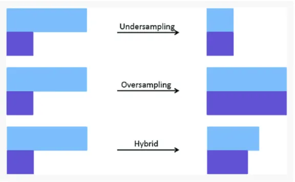
Sampling methods can be further categorized into oversampling and undersampling techniques and hybrid versions of them. Figure 3. illustrates their fundamental principles. On the left-hand side in Figure 3., the light blue bar represents the majority class, and the
dark blue the minority class. Undersampling techniques reduce the size of the majority class to the level of the minority class to fix the imbalance. Oversampling techniques take the opposite approach; the size of the minority class is increased. In oversampling tech-niques, new elements are added to the minority class based either on duplication or inter-polation. Hybrid solutions combine features from both undersampling and oversampling techniques. (Vluymans 2019.) If the training set is resampled to fix the imbalance, the test set should however be more nature-like to obtain reliable results. This means that if there is naturally a class imbalance in the data, the imbalance should not be fixed in the test data. (Kuhn & Johnson 2013.)
Figure 3. Sampling techniques (Vluymans 2019).
Synthetic Minority Oversampling Technique (SMOTE) is the most popular oversampling technique. It reinforces the minority class by generating new synthetic instances using linear interpolation between existing minority class instances and their nearest neighbors. Nearest neighbors mean in this case the data points, that are most similar with a given data point, measured with given features. (Vluymans 2019, Chawla et al. 2002.)
As stated above, sampling methods have been proven to be an effective way to handle the class imbalance. However, according to Kuhn & Johnson (2013), there is no one-above-others approach when it comes to sampling techniques. Being the most popular and easy to implement and interpret, SMOTE was chosen to be used in this thesis.
2.2.8 Evaluation metrics
There is a wide range of different ML models, designed to solve a variety of problems. Their functioning and characteristics often differ significantly, making it sometimes hard to evaluate, which one is performing best. In order to objectively evaluate the perfor-mance of a model, a consistent set of evaluation tools is required. In this section, some widely used tools for evaluating the performance of binary classification models are in-troduced6.
Accuracy is the simplest and perhaps the most used performance metrics. To calcu-late the accuracy score, the labels predicted by the trained model are compared to the known labels in the test data. Accuracy is thus the percentage of correct predictions made. The simplicity however brings some problems with it. Firstly, accuracy does not tell an-ything about the type or errors made during the process. In some tasks, this would be an important attribute, for some errors may be more severe than others. Secondly, accuracy does not take class imbalance into account. For example, if there are 50 instances of neg-ative class and 5000 instances of positive class in the data, the model would perform almost perfectly, if measuring only with accuracy. This happens, because almost all in-stances represent the positive class in the data. The model would then predict almost all of them to be positive, and therefore predict almost all of them correctly. Accuracy score would be high in this case, but little would be known about the performance on predicting the negative class. (Kuhn & Johnson 2013.) Thus, more versatile metrics are needed.
Figure 4. Confusion matrix (Adapted from Alpaydin 2014).
Confusion matrix (illustrated in Figure 4.) is a simple chart, where the observed classes can be arranged. It gives an overall picture of the performance of the model. In the matrix, a true positive (TP) is an observation correctly classified into the positive class, a false
6 The empirical part of this thesis focuses on binary classification. Therefore, it is reasonable to introduce only the evaluation metrics concerning it.
True class
Total
Positive
p
Negative
n
Total
N
Positive
TP: true positive
FP: false positive
p´
Predicted class
Negative
FN: false negative
TN: true negative
n´
positive (FP) an observation incorrectly classified into the positive class, a true negative (TN) an observation correctly classified into the negative class and a false negative (FN) an observation incorrectly classified into the negative class. P and n represent the total quantities of the true class instances, while p´ and n´ stand for the total quantities of cor-responding predictions. N is the total quantity of data. (Marsland 2014.)
Based on the results in the confusion matrix, following measurements can further be determined to help interpreting the performance of the model. Recall (also known as sen-sitivity and the true positive rate, equation 1) shows the amount of true positive instances, divided by all the positive instances in the data, while precision (equation 2) is the ratio of true positive instances divided by the quantity of all positive predictions made. To-gether, precision and recall give more information about the performance than accuracy. F1-score (equation 3) can be calculated as the harmonic mean of precision and recall. It gives a more holistic view on the performance of the model; such as accuracy, it does not make a distinction between the error types. (Marsland 2014.)
𝑅𝑒𝑐𝑎𝑙𝑙 = 𝑇𝑃 𝑇𝑃+𝐹𝑁 (1) 𝑃𝑟𝑒𝑐𝑖𝑠𝑖𝑜𝑛 = 𝑇𝑃 𝑇𝑃+𝐹𝑃
(2) 𝐹1 = 2 × 𝑝𝑟𝑒𝑐𝑖𝑠𝑖𝑜𝑛×𝑟𝑒𝑐𝑎𝑙𝑙 𝑝𝑟𝑒𝑐𝑖𝑠𝑖𝑜𝑛+𝑟𝑒𝑐𝑎𝑙𝑙 (3) Using the knowledge from the confusion matrix enables also a visual performance analysis. ROC (receiver operator characteristics) curve, illustrated in Figure 5., consists of true positive rate – false positive rate combinations. It describes the types of errors the classifier makes using different probability thresholds. The probability threshold means how sure the classifier needs to be to predict a certain class. Using different probability thresholds yields data points in the ROC space, and the ROC curve can then be specified through these points. Using the ROC curve analysis, it is possible to detect the types of errors the classifier is prone to make, and hence to tune the classifier to avoid the more severe types of errors. (Kuhn & Johnson 2013). The ideal classification model would draw a ROC curve, that goes through the point (0,1) (0% false positives, 100% true pos-itives). In contrast, the worst possible classifier would have a linear ROC-curve going through point (0,0) and (1,1). (James et al. 2013.) In order to wrap up the ROC curve
analysis to a single number, the AUC (area under the curve) can be calculated. An ideal classifier would have an AUC of 1.0, while the worst possible classifier would have an AUC of 0.5. Generally speaking, the closer the ROC curve is to the upper left corner of the plot in Figure 5., the better the performance of the model. (Alpaydin 2014.)
Figure 5. ROC-curve (James et al. 2013).
2.3 Natural language processing
NLP is a field concerned with technologies that enable computers to work efficiently with human language data. NLP is an interdisciplinary field; it combines techniques of linguis-tics, artificial intelligence, information engineering and computer science. NLP tasks in-clude enabling computers to understand human language, improving communication be-tween humans and other useful human speech or text processing tasks. The main objective in NLP applications is usually either understanding or producing human language. The focus of this thesis is in the former. (Hirschberg & Manning 2015, Cady 2017, Jurafsky & Martin 2018.)
To enable a computer to understand and analyze human language, the task needs to be split into smaller subtasks, that can be performed using special techniques. Various techniques can be implemented in NLP tasks. The relevant ones to this thesis are intro-duced in the following sections. An NLP analysis usually starts with text preprocessing.
2.3.1 Text preprocessing techniques
Tokenization is usually among the very first steps in most NLP tasks. Basically, tokeni-zation is separating a piece of text into smaller pieces (tokens), that are usually individual words. The separation is carried out using some predefined rules concerning for example spaces and certain punctuation marks. (Cady 2017.) Typically, in English language, a space separates two words from each other. There are however many exceptions (e.g. New York), where two consecutive words need to be treated as one entity (one token), in order the capture the correct meaning. In turn, sometimes an entity containing no spaces, needs to be separated into two tokens (e.g. I’m → I am). It is therefore crucial and some-times challenging to develop suitable rules for tokenization. (Jurafsky & Martin 2018.)
After the input text has been tokenized, a process called part-of-speech tagging (POS tagging) can be performed. In this process, a POS marker is assigned for each tokenized word in the corpus7. Since for most words the POS depends on the situation (e.g. “book”
can be a noun or a verb), the POS tagging process can be seen as a disambiguation pro-cess; the goal is to find the correct POS in a given context. Depending on the task, POS tagging is yet not always needed. It can be computationally expensive and thus its unnec-essary use should be avoided. (Jurafsky & Martin 2018.)
Techniques called stemming and lemmatization can be applied in order to unite dif-ferent variations of the same word. Their principal goal is similar, but they provide both different approaches and results. In lemmatization, the “lemma” of the word is its base
form. For example, “running”, “ran” and “runs” are all variations of the lemma “run”.
Thus, if the text in question is lemmatized, all the aforementioned words are turned into
“run”. The downside of lemmatization is its computational expense. In order to extract the lemma of the word, one also needs to define the POS for the word. This, as stated above, requires knowledge of the whole sentence surrounding the word. (Cady 2017.)
Stemming, in turn, is a more straightforward technique. It is computationally cheaper and easier to perform, but as a consequence, is usually less precise. The “stem” of the
word is simply a part of the word, obtained using predefined rules. Usually these rules strip off certain endings from words (e.g. “er” or “ing”). For example, the stem for words “producer”, “producing”, “product” and “production”, could be for example “produc-“.
In the “run” example used above, the words “running” and “ran” would be treated as separate words, if stemming was used. (Cady 2017.)
Along with stemming and lemmatization, the words are usually converted into low-ercase letters. For example, a word in the beginning of the sentence has its first letter written in uppercase. In further NLP analysis, this word, and the same word with all letters written lowercase, are treated as completely different words, regardless of the fact that they have the exact same meaning. (Uysal & Gunal 2014.) It is also common to remove certain punctuation marks from the text, sometimes all of them (Igual & Seguí 2017).
The removal of “stop words” is often a part of the preprocessing stage. One cannot unambiguously define which words are considered stop words, but generally words that do not contain much information themselves, are considered stop words. In English
lan-guage, for example, words “and”, “a”, “the”, “it” and “as” are usually treated as stop words, when preprocessing a piece of text. In many implementations, stop words are con-sidered as unnecessary noise only complicating the task, which justifies their removal. The implementer of an NLP analysis can define a list of stop words manually, or use a more general, pre-assembled list. In some occasions, certain words that are often consid-ered stop words, can be very meaningful. The removal of this kind of words will have a negative impact on the analysis. (Cady 2017.)
One preprocessing method worth consideration is the detection of synonyms and similar words. In the data, there usually appears several different words, that have a very similar meaning. Sometimes the analysis can be improved by collapsing all these words into a single identifier, a synset. This method is however problematic, because the mean-ing of the word often depends on the context, and therefore it can belong to many synsets. (Cady 2017.)
The goal of the above-mentioned techniques is, in essence, to convert the text into a more standard form; to normalize it. These techniques help to get rid of unnecessary and duplicate information. Appropriately used, they simplify the analysis and improve the results. (Jurafsky & Martin 2018). Their use always depends on the final objective of the analysis and the available data. Therefore, there is no exact guideline specifying when and how to use these techniques; usually the optimal solution must be found by experi-mentation. (Igual & Seguí 2017.)
2.3.2 Bag-of-words (BOW) and vectorization
After the textual data has been normalized using the above-introduced techniques, it can be turned into numerical vectors. In a vector form, the textual data is finally ready to be used as an input for an ML algorithm. In most NLP tasks, text documents are represented in a BOW format. This means that the positions of the words are ignored; only their fre-quency within the text is of interest. Basically, in the vectorization process, the dimension of the document vector is equal to the amount of individual words (or tokens) occurring in the entire corpus. Depending on their frequency, a weight is assigned for each word in the document. Hence, in the BOW concept, the text document can be represented as a vector in a (usually) high-dimensional word-space. Similarly, each word can be seen as a combination of relations to each document. (Jurafsky & Martin 2018, Cady 2017.)
The vectorization process can be visualized as a term-document (TD) matrix (Figure 13.). In Figure 6., the rows represent individual words, and how often they appear in
certain documents (columns). For instance, in the document “Julius Caesar”, the word
“battle” appears 7 times. These vectors are said to be count vectors; the vectors are created
simply by counting the word occurrences. Therefore, the weight for each word is obtained by counting its occurrences in the document. (Jurafsky & Martin 2018.)
Figure 6. A simple TD matrix (Jurafsky & Martin 2018).
This approach is however very limited. In most cases, some words are considered more important than others, and usually the most important words are not the most common ones. The count vector approach considers the most common words as the most im-portant, as their weights are the highest. A widely-used approach called TF-IDF (Term Frequency – Inverse Document Frequency) provides a solution for this problem. It basi-cally highlights rare words but lowers the weights for common words. (Cady 2017.) TF-IDF score 𝑤 for word 𝑡 in document 𝑑 is calculated the following way:
Where 𝑡𝑓𝑡,𝑑 is simply the frequency of the word in the document. It is usually weighted down by taking 𝑙𝑜𝑔10 of the frequency. Formally, 𝑡𝑓𝑡,𝑑 is given by:
𝑡𝑓𝑡,𝑑 = {1 + 𝑙𝑜𝑔10𝑐𝑜𝑢𝑛𝑡(𝑡, 𝑑) 𝑖𝑓 𝑐𝑜𝑢𝑛𝑡(𝑡, 𝑑) > 0
0 𝑜𝑡ℎ𝑒𝑟𝑤𝑖𝑠𝑒 (25)
𝑖𝑑𝑓𝑡, the inverse document frequency, is given by:
𝑖𝑑𝑓𝑡 = 𝑙𝑜𝑔10(𝑁
𝑑𝑓𝑡) (26)
Where N is the total number of documents in the corpus and 𝑑𝑓𝑡 tells how many docu-ments the word t occurs in. Thus, words that occur only in a few docudocu-ments are given a higher weight. To conclude, TF-IDF method assigns high importance for words that occur frequently in one document, but rarely in others. (Jurafsky & Martin 2018.)
Usually in a TF-IDF matrix, a minimum frequency constraint is applied. If a word occurs only very few times in a large document, its importance (TF-IDF score) gets inap-propriately high. Thus, only the words that occur at least, for example, five times in a document are included in the matrix. Even a minimum frequency constraint of two usu-ally excludes a lot of noise, for example typos, from the matrix. (Cady 2017.)
Instead of using only individual words, the above-mentioned techniques can be ap-plied also for so-called n-grams. An n-gram is a sequence of words, containing n words (n is the number of words). Often, words together construct a completely different ing comparing to individual words. The use of n-grams enables the capture of these mean-ings. In an NLP analysis, an n-gram is treated in the same way as an individual word. (Cady 2017.) Usually only two (bigram) or three (trigram) words long n-grams are used, because longer n-grams would form too large a TD matrix (Jurafsky & Martin 2018).
More generally, the text vectorization process is called feature extraction. That is, because the main goal of the vectorization process is to produce the features, that can be utilized as input data for a selected ML algorithm in the classification process. Usually, the vectors obtained in the vectorization process tend to be very sparse. The sparsity de-rives from the fact that usually a large number of words are involved in the corpus, but only a small fraction of the words appear in a single document. Therefore, most of the words in a document vector are assigned a weight of zero. A word, that is assigned a
weight of zero in many documents, is however not considered redundant or irrelevant, often quite the contrary. The goal of the above-introduced text preprocessing techniques can be seen as the removal of the redundant and irrelevant features from the analysis; to reduce the dimensionality of the TD matrix. (Elakiya & Rajkumar 2017.)
Even after careful preprocessing, lots of useless features typically remain in the TD matrix. A process called feature selection is implemented to select only the most informa-tive features for the classification stage. A basic approach to feature selection is to define some informativeness measure, rank all the features according to it, and eliminate some fixed amount of the most useless features. (Jurafsky & Martin 2018.)
2.3.3 Topic modeling
The dimensionality reduction of the TD matrix can be taken even further using a method called topic modeling. Topic modeling methods are a good example of unsupervised ML. The goal of topic modeling is to group all the words in the corpus into clusters of words, that occur frequently together. The formed clusters are intended to represent semantic or meaningful topics, giving an insight into the topical content of the corpus. In topic mod-eling, under the BOW assumption, the documents can be seen as a mixture of topics, where a topic is defined as a probability distribution over words. A topic model hence detects similar words in a document, groups them together into topics and outputs a dis-tribution over topics for the document. The topics can be further used as features in an ML model. (Steyvers & Griffiths 2007.)
According to Hajek et al. (2016) there are two general approaches to perform the dimensionality reduction of the TD matrix: latent semantic analysis (LSA) and probabil-istic topic models, for example latent dirichlet allocation. Both of these reduce the dimen-sionality of the TD matrix significantly, and therefore the number of features in the ML model. LSA is not officially an actual topic modeling technique, but it yields a functional and easy-to-interpret topical content analysis (Steyvers & Griffiths 2007, Hajek et al. 2016).
LSA constructs a semantic space of the TD matrix using singular value decomposi-tion (SVD). This allows the detecdecomposi-tion of the documents that contain similar topics, but different terms8. The SVD decomposes the TD matrix 𝐴 (m x n dimension) into a matrix
8 The above-introduced text preprocessing technique of removing synonyms and polysemy is partly an overlapping technique with LSA.
of document vectors 𝑉𝑇, a matrix of word vectors 𝑈 and Σ, a matrix of the singular values of 𝐴. The matrix factorization can be expressed by:
𝐴 = 𝑈 𝛴 𝑉𝑇 (27)
where 𝑈 (m x m dimension, m is the number of terms) and 𝑉𝑇 (n x n dimension, n is the number of documents) are orthogonal matrices and Σ (m x n dimension) is a diagonal matrix, where the singular values of the matrix 𝐴 are the diagonal values. The first r col-umns of the matrix 𝑈 (here r is the rank of the matrix) consist of r orthonormal eigenvec-tors determined by the r nonzero eigenvalues of 𝐴𝐴𝑇. The first r columns of the matrix V consist of r orthonormal eigenvectors determined by the r nonzero eigenvalues of 𝐴𝑇𝐴. So, in order to compute the SVD, the eigenvalues and eigenvectors of 𝐴𝐴𝑇 and 𝐴𝑇𝐴 have to be found. Here, the columns of 𝑈 are the eigenvectors of 𝐴𝐴𝑇 and the columns of 𝑉
are the eigenvectors of 𝐴𝑇𝐴. The common positive eigenvalues of 𝐴𝐴𝑇 and 𝐴𝑇𝐴 are the diagonal values of matrix Σ, and thus the singular values of 𝐴. Selecting the k largest singular values, and their corresponding singular vectors from 𝑈 and V yields a best rank k approximation to 𝐴. As a result, the dimensionality reduction from r to k removes the noise from the original matrix 𝐴 and captures the latent semantic structures in the data. The topics can be now determined by comparing the cosine similarities between the terms. Terms, that are near each other (have a high similarity) in the reduced k-dimen-sional space, have a similar meaning. Accordingly, documents, that are near each other share common topics. (Martin & Berry 2007, Hajek et al. 2016.)
3
RELATED LITERATURE
Machine learning has received a lot of attention during the last years, when it comes to forecasting purposes in finance. Numerous studies have been conducted on the prediction capabilities of ML methods, for example, in stock price movements and corporate bank-ruptcies. A state-of-art approach is to pick a few ML algorithms, implement them in the prediction task and compare the obtained results.
For instance, Shynkevich et al. (2017) used SVMs, artificial neural networks (ANN) and K-nearest neighbors (KNN) to predict stock price movements in the short term. The SVM model performed best with an accuracy of 75%, while accuracy obtained with the ANN model was slightly worse, 73%. Clearly the worst-performing model in the study was the KNN, with an accuracy of 60%. In turn, Barboza et al. (2017) achieved an accu-racy of 87% in predicting corporate bankruptcies, using a random forest model. It
outper-formed a more “traditional” logistic regression model, which achieved 69% accuracy.
Another popular prediction task in the financial sector is corporate credit ratings. The effect of financial ratios on credit ratings has been studied quite thoroughly. For example, Wu et al. (2014) used bagging combined with decision trees to achieve a credit rate clas-sification accuracy of 83%, using corporate financial statements as data. In addition, pop-ular methods for this kind of prediction task are, for example, SVMs (Kim & Ahn 2012, Chen & Li 2014), random forests (Yeh et al. 2012) and ANNs (Huang et al. 2004, Wallis et al. 2019).
In contrast to the above-mentioned approaches, the use of hidden information in com-pany-related textual content as predictor variables for credit rating classification is yet a relatively new and little researched concept. Hajek et al. (2016) combined the more tra-ditional approach, where only the financial ratios are used as predictor variables, with textual, topical content extracted from annual reports of U.S. companies (10-k form), for a credit rating classification task. They used TF-IDF to create a TD matrix and LSA to extract the hidden topics from it. Classification was performed using naïve Bayesian net-work, decision tree, random forest, SVM, multilayer perceptron, logistic regression and KNN. All of these classifiers were implemented on both the financial and the textual indicators, after which their results were combined. Without the financial indicators, the best-performing classifiers were logistic regression (AUC 0.907), SVM (AUC 0.862), multilayer perceptron (AUC 0.761) and naïve Bayesian network (AUC 0.728). Without the textual indicators, the best-performing classifiers were naïve Bayesian network (AUC
0.922), logistic regression (AUC 0.920), random forest (AUC 0.919) and multilayer per-ceptron (AUC 0.911). When the financial and textual indicators were combined, best classifiers were random forest (AUC 0.925), naïve Bayesian network (AUC 0.924), mul-tilayer perceptron (AUC 0.875) and SVM (AUC 0.870).
Without the financial indicators, the performance of the best-performing classifiers decreased significantly. This demonstrates their importance on credit rating classification tasks. The performance on only the financial indicators is almost as good as with all in-dicators. However, random forest and naïve Bayesian network, the best-performing clas-sifiers on all indicators decreased in performance, when the textual indicators were not used. This suggests that in the form 10-k annual reports, there might be some latent in-formation, useful for credit rating prediction.
Chen et al. (2017) compared the performance of different topic models and their abil-ities to predict bank failures. They used annual reports of U.S. companies in 8-k and 10-k forms as data. Ban10-k failure prediction performance on 10-10-k data was significantly worse than on 8-k data. They state that this derives from the high similarity of companies’ re-ports between consecutive years; the content within a 10-k report is typically mostly
cop-ied from the previous years’ corresponding document. A two-layer neural network was constructed for classification, achieving its best performance with latent dirichlet alloca-tion and 8-k data.
4
DATA AND METHODS USED IN THE STUDY
4.1 Form 10-k annual reports
The textual data used in this thesis is form 10-k annual reports of public U.S. companies from years 2000-2018. The U.S. Securities and Exchange Commission (SEC) requires all public U.S. companies to submit annual reports in form 10-k, after the company’s fiscal
year has ended. The deadline varies depending on the amount of the company’s public
float (60-90 days after the end of the fiscal year). Form 10-k reports contain plenty of
detailed information about the company’s latest fiscal year, allowing investors to be aware
of the company’s financial condition, before investing in it. (Sec.gov.)
The report is standardized and consists of four main sections, divided further into 20 subsections. Being a comprehensive report, a form 10-k is often very large, containing possibly hundreds of pages. (Sec.gov). Because of this, only three subsections, Item 1A (Risk factors), Item 7 (Management's discussion and analysis of financial condition and results of operations) and Item 7A (Quantitative and qualitative disclosures about market risks) were included in the data. These subsections are assumed to contain crucial infor-mation about the near future of the company. Therefore, it is assumed that one could predict a possible change in the company’s credit rating in the near future, on the basis of this information. In addition, according to Cohen et al. (2020), the content of 10-k annual reports generally varies very little between consecutive years. Chen et al. (2017) state this too; the cosine similarities between 10-k reports of consecutive years were very high. In Cohen et al. (2020), items 1A, 7 and 7A were found to have the most variation between consecutive years. Thus, they could be expected to contain the most predictive value, justifying their selection for this study. Chen et al. (2017) found also that another type of mandatory SEC filing, the form 8-k report, varies much more from year to year. As a consequence, predictions using 8-k data were also better. The use of 8-k data was consid-ered, but in a more standard format, 10-k data was found to be more suitable for this study.
4.2 Data preparation
The chosen subsections of form 10-k reports were downloaded from SEC’s EDGAR
da-tabase. Some companies submitted the desired subsections in a particular exhibit file. These files were also included in the data. The data was transferred to a Jupyter notebook,
where the data preparation and ML processes were convenient to perform, using Python programming language. The data preparation was started by deleting pure duplicate rows. Then, if there were two or more instances of the same subsection for a given company for a given year, the shorter one was deleted. Cases, where the content of the subsection referred to another document, was in a form of a data table or was non-informative in some other way, were also deleted. All the subsections for a given company for a given year were then merged, so that for a given company on a given year, the text data included all the available subsections.
The next step was to download public U.S. companies’ credit ratings for all those years, when the credit ratings had changed. First, if a company had received two or more ratings during one year, only the last rating of the year was included in the data, assuming that it represents the true creditworthiness of the company on that given year. After that, the rating values written in letters (e.g. AA+, CCC-), were replaced with numbers. Now, the direction of the credit rating change for a company could be determined with a simple subtraction. The credit rating change was then turned into a dummy variable, 1 represent-ing an increase in credit ratrepresent-ing and 0 representrepresent-ing a decrease.
After both tables had been prepared, one containing the text documents and other the credit ratings, the two tables were merged. The resulting table consisted of document-rating pairs for a given company for a given year (e.g. Microsoft’s documents for year 2004 and Microsoft’s credit rating for year 2004). For those documents that could not be
“matched” this way, a match was sought from the next years’ ratings, assuming that the information in the 10-k report could possible implicate a change in credit rating also one year after the corresponding 10-k report had been submitted. The total number of docu-ment-credit rating pairs construct this way was 1337.
4.3 Data limitations
After the above-mentioned preparations, the final quantities of the form 10-k subsections were: Item 1A: 1651, Item 7: 13406, Item 7A: 17163 and Exhibits: 2484. The number of
Item 1A’s is remarkably low, because only the biggest companies are required to submit
it. Thus, there are very few rows in the data, where all the subsections are included for a given company for a given year. The study could have been conducted using data
includ-ing, for example, only item 7A’s, but that would have shrunk the already limited data