A generic data representation for
predicting player behaviours
Hanting Xie
PhD
University of York
Computer Science
September, 2017
Abstract
A common use of predictive models in game analytics is to predict the behaviours of players so that pre-emptive measures can be taken before they make undesired decisions. A stan-dard data pre-processing step in predictive modelling includes both data representation and category definition.
Data representation extracts features from the raw dataset to represent the whole dataset. Much research has been done towards predicting important player behaviours with game-specific data representations. Some of the resulting efforts have achieved competitive perfor-mance; however, due to the game-specific data representations they apply, game companies need to spend extra efforts to reuse the proposed methods in more than one products. This work proposes an event-frequency-based data representation that is generally applica-ble to games. This method of data representation relies only on counts of in-game events instead of prior knowledge of the game. To verify the generality and performance of this data-representation, it was applied to three different genres of games for predicting player first-purchasing, disengagement and churn behaviours. Experiments show that this data-representation method can provide a competitive performance across different games.
Category definition is another essential component of classification problems. As labelling method that relies on some specific contions to distribut players into classes can often lead to imbalanced classification problems, this work applied two commonly used appraoches, i.e., random undersampling and Synthetic Minority Over-Sampling Technique (SMOTE), for rebalancing the imbalanced tasks. Results suggested that undersampling is able to provide better performance in the cases where the quantity of data is sufficient whereas the SMOTE has more chances when the dataset is too small to be balanced with the undersampling approach. Besides, this work also proposes a new category-definition method which can maintain a distribution of the resultant classes that is closer to balanced. In addition, the parameters used in this method can also be used to gain insight into the health of the game. Preliminary experimental results show that this method of category definition is able to improve the balance of the class distribution when it is applied to different games and provide significantly better performance than random classifiers.
Contents
1 Introduction 14
1.1 Motivations and Hypotheses . . . 14
1.2 Contributions . . . 16
1.2.1 Main Research Hypotheses . . . 16
1.2.2 Contribution Summary . . . 16
1.3 Outline . . . 17
2 Modelling with Data Mining 18 2.1 The ‘Data’ in Data Mining . . . 18
2.1.1 Game Telemetry . . . 19
2.1.2 Game Metrics . . . 19
2.1.3 Data Storage . . . 21
2.1.4 Data Attributes . . . 21
2.1.5 Data Cleaning . . . 22
2.1.6 Data Reduction and Data Representation . . . 23
2.2 Machine-learning based Data Mining . . . 26
2.2.1 Supervised Learning . . . 26
2.2.2 Unsupervised Learning . . . 28
2.2.3 Mining Association Rules . . . 28
2.3 Summary . . . 29
3 Game Data Mining 30 3.1 Modelling for Anomalous-behaviour detection . . . 31
3.2 Player Style Modelling . . . 32
3.3 Player Style-based AI . . . 33
3.4 Player Preference Learning and PCG (Procedure Content Generation) . . . . 34
3.5 Player Disengagement Modelling . . . 35
3.6 Player-purchase Modelling . . . 38
3.7 Generic Feature Extraction . . . 39
3.8 Summary . . . 42
4 Player Modelling with Data Mining 43 4.1 A Glance at The Research . . . 43
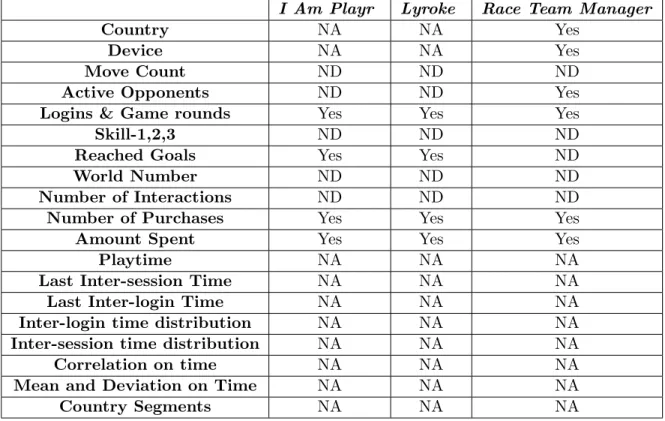
4.2 Game-data Sources . . . 44
4.2.1 I Am Playr . . . 44
4.2.2 Lyroke . . . 46
4.2.3 Race Team Manager . . . 47
4.3 Labelling Methods . . . 48 3
4.4 Balancing Methods . . . 48
4.5 Data Representation . . . 48
4.5.1 Event Frequency-based data representation . . . 48
4.5.2 Game Specific Data Representation . . . 50
4.6 Feature Selection . . . 51
4.7 Classification Algorithms . . . 51
4.8 Evaluation Methods . . . 52
4.8.1 Confusion Matrix . . . 52
4.8.2 Top-level Measurements . . . 53
4.9 Overfitting and K-fold Cross-validation . . . 56
4.10 Summary . . . 58
5 Predicting First Purchase 61 5.1 First Purchase . . . 61
5.2 First-purchase prediction . . . 62
5.2.1 Experiment Information . . . 62
5.2.2 Experiment Details and Results . . . 65
5.2.3 Discussion . . . 68
5.3 First-purchase Prediction with Feature Selection . . . 71
5.3.1 Experiment Information . . . 73
5.3.2 Experiment Details and Results . . . 73
5.3.3 Discussion . . . 76
5.4 Conclusion . . . 77
6 Predicting Disengagement 78 6.1 Disengagement Prediction with Event-frequency-based Data Representation . 79 6.1.1 Experiment Information . . . 79
6.1.2 Experiment Details and Results . . . 81
6.1.3 Summary . . . 83
6.2 Disengagement Prediction with Event-frequency-based Data Representation with Feature Selection . . . 84
6.2.1 Experiment Information . . . 84
6.2.2 Experiment Details and Results . . . 86
6.2.3 Summary . . . 89
6.3 Disengagement Prediction with Event-frequency-based and Game-specific Data Representation . . . 89
6.3.1 Experiment Information . . . 90
6.3.2 Experiment Details and Results . . . 91
6.3.3 Summary . . . 94
6.4 Churn Prediction . . . 94
6.4.1 Experiment Information . . . 95
6.4.2 Experiment Details and Results . . . 97
6.4.3 Summary . . . 102
CONTENTS 5
7 Biased Player Behaviour Modelling 105
7.1 Bias in Data Mining . . . 105
7.2 Disengagement prediction – Biased . . . 106
7.2.1 Experiment Information . . . 106
7.2.2 Experiment Details and Results . . . 107
7.2.3 Summary . . . 110
7.3 First-purchase prediction – Biased . . . 111
7.3.1 Experiment Information . . . 111
7.3.2 Experiment Details and Results . . . 111
7.3.3 Summary . . . 114
7.4 Churn prediction – Biased . . . 114
7.4.1 Experiment Information . . . 115
7.4.2 Experiment Details and Results . . . 115
7.4.3 Summary . . . 117
7.5 SMOTE Balancing . . . 118
7.6 Disengagement Prediction – SMOTE . . . 121
7.6.1 Summary . . . 125
7.7 Churn Prediction – SMOTE . . . 125
7.7.1 Summary . . . 129
7.8 Conclusion . . . 131
8 Conclusion 133 8.1 Contributions . . . 133
8.1.1 Main Research Hypothesis . . . 133
8.1.2 Contribution Summary . . . 133
8.2 Limitations . . . 135
8.3 Future Work . . . 136
8.4 Closing Remarks . . . 137
Appendices 138 A Disengagement Over Varying Dates 139 A.1 Definition . . . 139
A.2 Insights from parameters . . . 139
A.3 Experiment Details and Results . . . 140
List of Tables
2.1 Types of Attributes . . . 22
2.2 Example of item set . . . 29
4.1 I Am Playr Data Example . . . 45
4.2 Lyroker Data Example . . . 46
4.3 Race Team Manager Data Example . . . 47
4.4 Example event explanation . . . 50
4.5 Event Frequency Data Representation . . . 50
4.6 Parameter Selection Ranges for Algorithms Applied . . . 52
4.7 Confusion Table . . . 53
4.8 A brief summary of measurements being applied in this work . . . 57
5.1 The availability of the game-specific features used in the study by Sifa et al. (2015) in the three games of this research . . . 63
5.2 Performance for predicting first-purchase behaviours with event-frequency-based data representation of the dataset ofI Am Playr (balanced by random undersampling) . . . 66
5.3 Performance for predicting first purchase behaviours with event frequency based data representation on the dataset ofLyroke (Balanced by the random undersampling method) . . . 67
5.4 Performance for predicting first purchase behaviours with event frequency based data representation on the dataset of Race Team Manager (Balanced by the random undersampling method) . . . 68
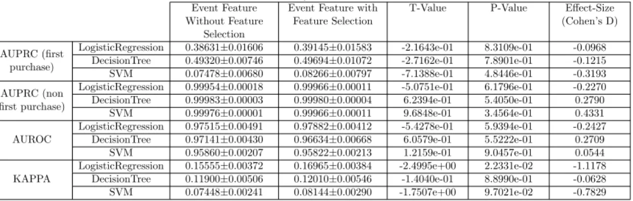
5.5 Performance for predicting first-purchase behaviours with event-frequency-based data representation (with and without feature selection) on the dataset ofI Am Playr (balanced by the random-undersampling method) . . . 73
5.6 Equivalence testing on the performance for predicting first-purchase behaviours with event-frequency-based data representation (with and without feature se-lection) on the dataset ofI Am Playr (balanced by the random-undersampling method) . . . 74
5.7 Performance for predicting first-purchase behaviours with event-frequency-based data representation (with and without feature selection) on the dataset ofLyroke (balanced by the random-undersampling method) . . . 75
5.8 Equivalence testing on the performance for predicting first-purchase behaviours with event-frequency-based data representation (with and without feature se-lection) on the dataset of Lyroke (balanced by the random-undersampling method) . . . 75
LIST OF TABLES 7
5.9 Performance for predicting first-purchase behaviours with event-frequency-based data representation (with and without feature selection) on the dataset ofRace Team Manager (balanced by the random-undersampling method) . . 76 5.10 Equivalence testing on the performance for predicting first-purchase behaviours
with event-frequency-based data representation (with and without feature se-lection) on the dataset of Race Team Manager (balanced by the random-undersampling method) . . . 77 6.1 Performance for predicting disengagement behaviours with
event-frequency-based data representation on the dataset ofI Am Playr (balanced by random undersampling) . . . 81 6.2 Performance for predicting disengagement behaviours with
event-frequency-based data representation on the dataset ofLyroke (balanced by random un-dersampling) . . . 82 6.3 Performance for predicting disengagement behaviours with
event-frequency-based data representation on the dataset of Race Team Manager (balanced by random undersampling) . . . 83 6.4 Performance for predicting disengagement behaviours with
event-frequency-based data representation (with and without feature selection) on the dataset ofI Am Playr (balanced by random undersampling) . . . 86 6.5 Equivalence testing on the performance for predicting disengagement behaviours
with event-frequency-based data representation (with and without feature se-lection) on the dataset ofI Am Playr (balanced by the random-undersampling method) . . . 87 6.6 Performance for predicting disengagement behaviours with
event-frequency-based data representation (with and without feature selection) on the dataset ofLyroke (balanced by random undersampling) . . . 88 6.7 Equivalence testing on the performance for predicting disengagement behaviours
with event-frequency-based data representation (with and without feature se-lection) on the dataset of Lyroke (balanced by the random-undersampling method) . . . 88 6.8 Performance for predicting disengagement behaviours with
event-frequency-based data representation (with and without feature selection) on the dataset ofRace Team Manager (balanced by random undersampling) . . . 89 6.9 Equivalence testing on the performance for predicting disengagement behaviours
with event-frequency-based data representation (with and without feature se-lection) on the dataset of Race Team Manager (balanced by the random-undersampling method) . . . 90 6.10 The availability of the game-specific features used in the study by Runge et al.
(2014) . . . 91 6.11 Performance for predicting disengagement behaviours with both
event-frequency-based and a game-specific data representation on the dataset of I Am Playr (balanced by random undersampling) . . . 92 6.12 Performance for predicting disengagement behaviours with
event-frequency-based and game-specific data-representation methods on the dataset ofLyroke (balanced by random undersampling) . . . 93
6.13 Performance for predicting disengagement behaviours with event-frequency-based and game-specific data-representation methods on the dataset of Race Team Manager (balanced by random undersampling) . . . 94 6.14 Performance for predicting churn behaviours with both event-frequency-based
and a game-specific data-representation methods for the dataset ofI Am Playr (balanced by random undersampling) . . . 98 6.15 Performance for predicting churn behaviours using both event-frequency-based
data representation (balanced by random undersampling) and a random guess on the dataset of I Am Playr . . . 98 6.16 Performance for predicting churn behaviours using both game-specific data
representation (Balanced by random undersampling) and a random guess on the dataset ofI Am Playr . . . 99 6.17 Performance for predicting churn behaviours with event-frequency-based and
a game-specific data representation on the dataset of Lyroke (balanced by random undersampling) . . . 100 6.18 Performance for predicting churn behaviours with both event-frequency-based
data representation (balanced by random undersampling) and a random guess at the dataset ofLyroke . . . 100 6.19 Performance for predicting churn behaviours with both the game-specific data
representation (balanced by random undersampling) and a random guess on the dataset ofLyroke . . . 101 6.20 Performance for predicting churn behaviours using event-frequency-based and
game-specific data representations on the dataset ofRace Team Manager (bal-anced by random undersampling) . . . 101 6.21 Performance for predicting churn behaviours with both the event data
repre-sentation (balanced by random undersampling) and a random guess on the dataset ofRace Team Manager . . . 102 6.22 Performance for predicting churn behaviours using both event-data
repre-sentation (balanced by random undersampling) and a random guess on the dataset ofRace Team Manager . . . 102 7.1 Performance for predicting disengagement behaviours with
event-frequency-based data representation on the dataset of I Am Playr (with and without balancing) . . . 107 7.2 Performance for predicting disengagement behaviours with
event-frequency-based data representation on the dataset ofLyroke(with and without balancing)108 7.3 Performance for predicting disengagement behaviours with
event-frequency-based data representation on the dataset of Race Team Manager (with and without balancing) . . . 109 7.4 Performance for predicting first-purchasing behaviours with
event-frequency-based data representation on the dataset of I Am Playr (with and without balancing) . . . 112 7.5 Performance for predicting first-purchasing behaviours with event
frequency-based data representation on the dataset ofLyroke(with and without balancing)113 7.6 Performance for predicting first-purchasing behaviours with
event-frequency-based data representation on the dataset of Race Team Manager (with and without balancing) . . . 114
LIST OF TABLES 9
7.7 Performance for predicting churn behaviours with event-frequency-based data representation on the dataset of I Am Playr (with and without balancing) . . 116 7.8 Performance for predicting churn behaviours with event-frequency-based data
representation on the dataset of Lyroke (with and without balancing) . . . . 117 7.9 Performance for predicting churn behaviours with event-frequency-based data
representation on the dataset ofRace Team Manager (with and without bal-ancing) . . . 118 7.10 The specifications of the server for running the experiments . . . 120 7.11 Performance for prediction disengagement with SMOTE on the dataset of I
Am Playr . . . 122 7.12 Performance for prediction disengagement with SMOTE or undersampling on
the dataset ofI Am Playr . . . 122 7.13 Performance for prediction disengagement with SMOTE on the dataset of
Lyroke . . . 123 7.14 Performance for prediction disengagement with SMOTE or undersampling on
the dataset ofLyroke . . . 123 7.15 Performance for prediction disengagement with SMOTE on the dataset of
Race Team Manager . . . 124 7.16 Performance for prediction disengagement with SMOTE or undersampling on
the dataset ofRace Team Manager . . . 124 7.17 Performance for prediction churn with SMOTE on the dataset of I Am Playr 127 7.18 Performance for prediction churn with SMOTE or undersampling on the
dataset ofI Am Playr . . . 127 7.19 Performance for prediction churn with SMOTE on the dataset of Lyroke . . 128 7.20 Performance for prediction churn with SMOTE or undersampling on the
dataset ofLyroke . . . 128 7.21 Performance for prediction churn with SMOTE on the dataset ofRace Team
Manager . . . 129 7.22 Performance for prediction churn with SMOTE or undersampling on the
dataset ofRace Team Manager . . . 129 A.1 Performance for Comparisons on Disengagement Over Varying Dates on the
dataset ofI Am Playr . . . 141 A.2 Performance for Comparisons on Disengagement Over Varying Dates on the
dataset ofLyroke . . . 142 A.3 Performance for Comparisons on Disengagement Over Varying Dates on the
List of Figures
2.1 The Subcategories in Player Metrics (Drachen et al., 2013) . . . 20
2.2 The idea of SVD (Barbar’a et al., 1997) . . . 25
2.3 Supervised Learning . . . 27
2.4 Unsupervised Learning . . . 28
4.1 Structure of research experiments . . . 44
4.2 Screenshot of I Am Playr . . . 45
4.3 Screenshot of Lyroke . . . 46
4.4 Screenshot of Race Team Manager . . . 47
4.5 Problem for calculating session length . . . 49
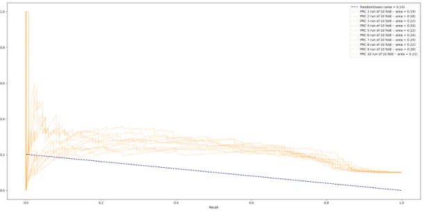
4.6 PRC curves for 10-fold cross validation while predicting disengagement with the event frequency based data representation . . . 55
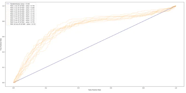
4.7 ROC curve for 10-fold cross validation while predicting disengagement with the event frequency based data representation . . . 56
4.8 Overfitting Problem . . . 57
5.1 Experiment of First Purchase Prediction . . . 62
5.2 Examples of Players in Making First Purchase Class . . . 64
5.3 Examples of Players in Non First Purchase Class . . . 65
5.4 The number of cases where methods achieve significantly better performance and the number of cases where there is no difference found for predicting first purchasing behaviours . . . 69
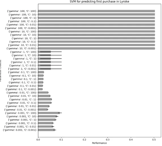
5.5 Investigation of SVM in I Am Playr for Predicting First Purchase . . . 70
5.6 Investigation of SVM in Lyroke for Predicting First Purchase . . . 71
5.7 Investigation of SVM in Race Team Manager for Predicting First Purchase . 72 5.8 Experiment of First-purchase prediction . . . 72
6.1 Experiment of First-purchase prediction . . . 79
6.2 The number of cases where methods achieve significantly better performance and the number of cases where there is no difference found for predicting disengagement behaviours . . . 84
6.3 The number of cases where methods achieve significantly better performance and the number of cases where there is no difference found for predicting churn behaviours . . . 85
6.4 Experiment of First Purchase Prediction . . . 85
6.5 Experiment of Disengagement Prediction . . . 91
LIST OF FIGURES 11
6.6 The number of cases where methods achieve significantly better performance and the number of cases where there is no difference found for predicting disengagement behaviours . . . 95 6.7 Experiment of First-purchase prediction . . . 96 6.8 Churn Definition by Runge et al. (2014) . . . 97 6.9 The number of cases where methods achieve significantly better performance
and the number of cases where there is no difference found for predicting churn behaviours . . . 103 7.1 Balancing Investigation Experiment of Disengagement Prediction . . . 107 7.2 The number of cases where methods achieve significantly better performance
and the number of cases where there is no difference found for predicting disengagement behaviours with undersampling . . . 110 7.3 Balancing Investigation Experiment of First Purchase Prediction . . . 111 7.4 The number of cases where methods achieve significantly better performance
and the number of cases where there is no difference found for predicting first purchase behaviours with undersampling . . . 115 7.5 Balancing Investigation Experiment of Churn Prediction . . . 116 7.6 The number of cases where methods achieve significantly better performance
and the number of cases where there is no difference found for predicting churn behaviours with undersampling . . . 119 7.7 On the left, when the classes can be linearly separated, SMOTE is able to
generate new synthetic data in the right place. However, when the classes can only be split by a non-linear classifier, SMOTE may create new synthetic data on the wrong side. . . 120 7.8 SMOTE Investigation Experiment of Disengagement Prediction . . . 122 7.9 The number of cases where methods achieve significantly better performance
and the number of cases where there is no difference found for predicting disengagement behaviours with SMOTE . . . 125 7.10 The number of cases where methods achieve significantly better performance
and the number of cases where there is no difference found for predicting disengagement behaviours with SMOTE and undersampling . . . 126 7.11 SMOTE Investigation Experiment of Churn Prediction . . . 127 7.12 The number of cases where methods achieve significantly better performance
and the number of cases where there is no difference found for predicting churn behaviours with SMOTE . . . 130 7.13 The number of cases where methods achieve significantly better performance
and the number of cases where there is no difference found for predicting churn behaviours with SMOTE and undersampling . . . 131 A.1 Experiment of Disengagement Over Varying Dates Prediction . . . 140
Acknowledgements
I would first like to thank my thesis supervisor Prof. Daniel Kudenko and Dr. Sam Devlin of the University of York. They helped me so much not only on my research but also constantly giving me tons of suggestions to my PhD life and career skill development.
I would also like to thank Prof. Peter Cowling who gave me lots of helpful advices on my first publication during my PhD.
I would also like to acknowledge Mr. Alex Whittaker at Inspired Gaming Ltd. who gave me permissions to the data of their games for finishing my PhD Research. Similarly, Mr. Neil Hutchinson at Bigbit Ltd. who granted me permissions to work with the data of their games, too.
Finally, I must express my very profound gratitude to my wife and my parents for pro-viding me with continuous encouragement throughout my years of study and through the process of researching and writing this thesis. This accomplishment would not have been possible without them. Thank you.
Declaration
I declare that this thesis is a presentation of original work and I am the sole author. This work has not previously been presented for an award at this, or any other, University. All sources are acknowledged as References.
Introduction
1.1
Motivations and Hypotheses
The digital-game industry is one of the fastest growing industries in the world, with over 1500 new products published annually (Bauckhage et al., 2012). Due to the limitations of past technologies, data analytics was not commonly involved in the process of developing games. Most games were played off-line, such that their data could hardly be collected. This fact, however, has dramatically changed in recent decades because of the rapid spread of the Internet. Nowadays, because most games are played with the Internet connected across a variety of devices, an enormous number of player behaviours can be collected via telemetry methods. However, since the raw data collected is often noisy and massive, it is hard to extract useful information.
Data analytics has been heavily used in recent years to address this issue. Instead of providing only statistical descriptions of players to inform better decision making, data mining, an important element of data analytics, can make forecasts of important behavioural trends such that risks (e.g., the disengaging trends of some players) and opportunities (e.g., the trend that some players will become paying users) may be noted in advance (Yannakakis et al., 2013).
With the rapid growth of both data-driven game development and data-mining tech-nology, several works have applied data-mining approaches to such tasks as anomalous be-haviour detection (Ahmad et al., 2009; Kang et al., 2012; Laurens et al., 2007; Mitterhofer et al., 2009; Woo et al., 2012), player preference modelling (Charles and Black, 2004; Hu-nicke and Chapman, 2004; Missura and G¨artner, 2009; Pedersen et al., 2010; Shaker et al., 2010; Togelius et al., 2007, 2011; Yannakakis and Togelius, 2011), player-preference based AI characters (Aiolli and Palazzi, 2008; Bakkes et al., 2009; Bauckhage et al., 2003; Cowling et al., 2015), player-disengagement prediction (Borbora et al., 2011; Borbora and Srivastava, 2012; Debeauvais et al., 2014; Drachen et al., 2016; Hadiji et al., 2014; Kawale et al., 2009; Runge et al., 2014; Tarng et al., 2009) and player-purchasing prediction (Pluskal and ˇSediv´y, 2014; Sifa et al., 2015). Approaches introduced in these works effectively predict the targets in the games in which they conducted the experiments; however, the common problem is the data-representation methods applied in these works can hardly be made generic. In the process of data mining, the data-representation stage aims to transform the raw dataset into a vectorised information format which is ready for training machine-learning models. In this format, each vector (also referred to as afeaturein data mining) represents one or a combina-tion of more attributes in the original unprocessed dataset. Therefore, decisions concerning how to construct these features are often important and can affect the performance of
CHAPTER 1. INTRODUCTION 15
tant classifiers. In most of the methods proposed in these works, the limitation of generality on data representation comes either from the game-specific vectors selected or from a lack of availability of some features in new games. Specifically, this happens when predictions are made based on game-specific data representations which use game events that appear only in a specific type of game (e.g., how many enemies killed in a war game), whereas the latter issue arises when some features are general enough but are not tracked in some games.
To solve the generality issue of the existing methods, this work introduces (as the main contribution) a generic data-representation method called event-frequency-based data rep-resentation, which can be migrated to build feature spaces in different games without any prior knowledge of them. Instead of extracting specific information from the game dataset for each player, this approach takes counts of all of the in-game events that happen to (or are generated by) this player as the data representation. In this way, the actual meanings of the events become less important. This is also why this data-representation method can be seamlessly migrated to different game products with minor modifications.
Apart from this issue, which exists in the stage of creating the data representation for training classifiers, another common issue that can be found in many existing works is the imbalanced dataset. Because the predictions of players’ future behaviours is a classification task in machine learning (e.g., whether a player will be leaving the game in the near future or not), a labelling method is needed to describe the task and to distribute players into their corresponding classes for predictive purposes. While labelling methods often use some specific conditions to distinguish players, an imbalanced class distribution can easily be created if the majority of players can satisfy the defined conditions. Unfortunately, an imbalanced classification task may lead to imbalanced classifiers.
In this work, two existing approaches are used to solve the imbalance issues found in three commercial games. Experiments show that both methods are able to help only in some cases. This suggests that, when a dataset is biased by some labelling method, a balancing method might help but that stable improvement is not guaranteed. In addition, some labelling methods might sometimes also lead to small datasets which can hardly be used for training higher-dimensional classifiers. In this study, when the predictive purpose is to forecast churn behaviours, the dataset labelled by the churn-labelling method is not only small (lacking data samples); it also shows a distribution bias in some games. To deal with this type of issue, this work applied two existed balancing methods and reviewed their abilities for dealing with the bias issues in this research. This work also offers a new labelling method called disengagement over varying dates. This labelling method is close to the concept of churn, which also aims to predict players’ disengagement behaviours, but it can maintain an approximately balanced distribution while labelling. In addition, this method also comes with two parameters that can be used to provide insight into the health of a game. Preliminary results for investigating the ability of this research can be found in Appendix A.
This section explains the current status of this research area and the challenges it faces. A basic introduction has been given of the research motivations and main contributions of this study. To investigate and verify the main contributions, several experiments were conducted that made extra contributions in different parts of the study. The next section identifies all the contributions made by this work.
1.2
Contributions
1.2.1 Main Research Hypotheses
As introduced in Section 1.1, this study offers a generic data-representation method for pre-dicting player behaviours that is designed to work across different games. To investigate its utility, the following research hypothesis was proposed: Event-frequency-based data representation can be used to predict player behaviour with supervised learning to provide a significantly better performance than random guess and competi-tive performance while being compared to other state-of-the-art methods, where applicable. Detailed explanations of this hypothesis can be found in Section 4.5.1.
1.2.2 Contribution Summary
To test both of the main research hypotheses proposed in Section 1.2.1, several contributions have been made during this research. A summary is given in this section to introduce their content.
Event Frequency-based data Representation
As the main contribution of this work, a generic data-representation method is proposed which can form the feature space only on the counts of events created (or experienced) by players. Because counts of events are content irrelevant, this data-representation method can be smoothly migrated to a wide range of different game products for predicting player behaviours. This corresponds to first main research hypothesis stated in Section 1.2.1. Details of it can be found in Section 4.5.1.
Player First Purchase Behaviour Prediction
To test the hypothesis, this work applies event-frequency-based data representation to predict players’ first-purchase behaviours in three different commercial games. It achieved significantly better performance than a random classifier. Details of this experiment can be found in Chapter 5.
Disengagement Labelling Method A new labelling method named ‘disengagement’ is proposed in this study which represents the disengaging behaviour of players. Unlike the commonly applied labelling method called ‘churn’, this method focuses on predict-ing players’ disengagpredict-ing trends instead of their exact leavpredict-ing actions. Developers would have more time to retain players by using extra care because the player has not yet decided to leave the game. Further details of this labelling method can be found in Section 6.1.1.
Player Disengagement/Churn Behaviour Prediction
The event-frequency-based data-representation method are used to predict the play-ers’ disengagement and churn behaviours to verify the hypothesis. Experiments show comparisons of classifiers trained with this data-representation method and another state- of-the-art game-specific data-representation method. Further information about the experiments is offered in Chapter 6.
An Evaluation of Two Popular Class Balancing Methods
Imbalanced class distribution is another issue that is often seen not only in game data-mining problems but also in other data-data-mining research areas. This work discusses the general causes of imbalanced class distribution using two methods that are commonly
CHAPTER 1. INTRODUCTION 17
used to solve this type of issue: random undersampling andSMOTE (synthetic minority over-sampling technique). Statistical comparisons are given to show that the random undersampling and SMOTE methods would help improve the performance of classifiers. Details of these comparisons can be found in Chapter 7
Disengagement Over Varying Dates Labelling method
Based on experiments in which datasets labelled with the churn definition are not large enough and are sometimes biased for training higher-dimensional data representation, this work proposes a new, alternative labelling method that aims to use all data sam-ples while maintaining an approximately balanced dataset. This alternative can help to solve two common issues discovered in this research: imbalanced and small data samples. In addition, parameters optimised for balancing in this method can be used as indicators of the game’s health. Preliminary results have shown classifiers trained in tasks balanced by this method can perform significantly better than random classifiers. Further details of it are covered in Appendix A.
1.3
Outline
This thesis is organised as follows:
1. First,a basic introduction to machine learning and data mining is given. At the same time, several types of metrics are explained that are collected in the game context. 2. Next, a literature review is given of several studies that have attempted to predict
various player behaviours. The data-representation methods applied in these works are discussed in detail.
3. Afterwards, before diving into experiments, the research methods are discussed. This section includes a global view of all the consequent experiments.
4. To investigate the utility of event-frequency-based data-representation methods for predictive tasks, it is first used to predict decisions regarding first purchases in three commercial games of different genres.
5. In addition, this data-representation method is utilised to predict players’ disengage-ment. During this experiment, some limitations of the event-frequency-based data-representation methods are discussed.
6. After the event-frequency-based data-representation method has been tested, another common issue–the imbalanced dataset, which was discovered while conducting these experiments–is introduced. Some explanations are given that will enable us to work out the possible cause of it, and some existing methods are applied to rebalance the dataset. A possible solution called disengagement over varying dates is also introduced as an alternative to deal with this type of problem. Experiments show that classifiers trained under balanced datasets can perform significantly better than a random classifier. 7. Finally, the conclusion is given to summarise the contribution of this work. Based
on some limitations introduced earlier, further work that may be conducted is also introduced.
Modelling with Data Mining
From games (Mahlmann et al., 2010) and films (Saraee et al., 2004) to serious areas like earthquake prediction (Otari and Kulkarni, 2012) and medical diagnosis (Soni et al., 2011), an increasing number of areas have entered the century of fast growing information. A very large amount of data is generated every second. According to Hilbert (Hilbert, 2013), in an average minute in 2012, around 2,000 search queries were received by Google, nearly 700,000 pieces of content were shared by Facebook users and almost 100,000 tweets were produced by Twitter users. Although data generated in these areas can occur in different formats, a common problem they face is that the data has been grown so massive that cannot be easily analysed. As mentioned in Chapter 1, data mining is considered as one of the most reliable ways for digging meaningful patterns from a very large amount of data.
This chapter offers an introduction to how and what type of game data is commonly collected in state-of-the-art methods. Next, the basics of data mining (including machine learning) are reviewed. This introduction covers most important aspects of how data is processed before and during analysis. Main points in this chapter:
u an overview of the data in games,
u descriptions about data cleaning,
u review of the dimensional reduction methods, and
u review of the machine learning based data mining process.
2.1
The ‘Data’ in Data Mining
As discussed above, since databases have become extremely large, it has never been more difficult to extract valid information from them. Data mining, also referred to as knowl-edge discovery from data (KDD), is a promising technology that aims to summarize latent patterns/models and discover unsuspecting relationships in databases by applying both sta-tistical approaches and machine-learning algorithms (Han and Kamber, 2011; Hand et al., 2001). As datasets have become increasingly massive, it is important to make sure that the data quality is good enough before a data-mining method is applied. This section dis-cusses the data types that are generally collected and used for behaviour modelling. Next, it discusses basic data-relevant concepts and how data can be cleaned and simplified.
CHAPTER 2. MODELLING WITH DATA MINING 19
2.1.1 Game Telemetry
This section offers a basic explanation is given of what data types are generally used for player behaviour-predictive modelling. According to Drachen (Drachen et al., 2013), game telemetry is a method whereby developers can collect game data from player clients over a distance. In the modern game industry, it has become the most widely used method for collecting game data (Zoeller, 2013) from free-to-play games and even ‘AAA’ titled games. This is because a game-telemetry system can help a game company not only track the real-time performance of a game but also record players’ historical behaviours to storage databases. As introduced by Weber (Weber et al., 2011a), the conventional way to implement the system is to integrate a client or basic collection logical codes into games and transmit data to a collection server. Depending on the preferences of different companies, the data collected might be either formatted or kept raw in the server for the convenience of further analysis. While transmitting data to collection servers, because exhaustively recording player behaviours’ in every frame could easily lead to very large cost and heavy transition pressures, the widely used approach (e.g, used by Google Analytics, Yahoo Flurry, Game Analytics, Unity, Upsight and Game Sparks) is to transmit data based on the firings of in-game events. In other words, the game data is only be transmitted in accord with pre-defined, in-game events. Generally, these events are in-game actions or behaviours, chosen by developers, which should be able to reflect any update on the status of games and milestones players achieved. Therefore, it is crucial to design an optimal and informative game-telemetry system. In most cases, the development of a game-telemetry system is comprised of at least two elements: game metrics, data storage.
2.1.2 Game Metrics
To perform game analysis, data collected from telemetry would normally be transformed into a more interpretable format defined asgame metrics. For example, in a shooting game, some samples of game metrics are logs of a player’s shootings behaviours, hitting rate, weapon preferences, average number of bullets used for killing an enemy and so on. This can be different in a racing game in which metrics can include players’ movements, final positions, items used, etc. In other words, game metrics can vary based on game type and game content. Therefore, generic game data that can be found in all types of games is generally limited.
As introduced by Drachen (Drachen et al., 2013), game metrics can include three types: player metrics, process metrics and performance metrics. Of these, process metrics and performance metrics are more beneficial for adjusting system development and performing bug fixes than for game-analytics purposes. Player metrics stands for all data related to players’ behaviours and gameplay tracks. This is the main sort of metric that game analytics is applied to. The definitions ofplayer metricscan be further split into subcategories (shown in Figure 2.1). The definitions are as follows:
Customer Metrics
Transactions are commonly seen in modern free-to-play games, and it is necessary to track the details of each transaction. Associated with player identity, this type of log could include in-game/out-game payments for game time, products and any items in the game. An example application of this can be found in the work of (Lim and Harrell, 2013) which uses players’ preferences for hats (an item) in the game, Team Fortress 2 (Valve, 2007), to investigate taste performances.
Figure 2.1: The Subcategories in Player Metrics (Drachen et al., 2013)
Community Metrics
This type of metric is able to reflect social interactions among players in a game. It is common for modern games to integrate some social networks, whether third-party platforms (e.g., Facebook and Twitter) or game-specific platforms (e.g., guilds inWorld of Warcraft). These metrics help researchers/developers gain a better understanding of the behaviours in a social group rather than of individuals. For example, Thurau and Bauckhage (2010) investigated the evolution patterns of guilds (a form of community) in the game, World of Warcraft (Blizzard, 2004). At the same time, these metrics can also be used to find similar styles among players in games. As an example of this, Kirman and Lawson (2009) discuss how social communities in online games could be utilised for identifying play styles.
Gameplay Metrics
Gameplay metrics is an important sub-category which represents most general in-game behaviours. This can be further broken down into interface metrics, in-game metrics and system metrics.
Interface metrics describe how players interact with the interfaces of a game. For example, in the main menu of games, metrics are collected concerning which options are used most by players and what purposes they use them for.
In-game metrics show how players behave in a game. This category is comprised of any metrics that are related to players’ behaviours during gameplay. It can help to reflect players’ skills, activities and preferences. For example, Pederson studied how to model players’ experience in Infinite Mario Bros (Markus-Persson, 2008) by using in-game metrics such as death rate, jump times and so on (Pedersen et al., 2009). System metrics record the system status corresponding to operations by players. Level settings provide an example. Shaker et al. (2010) looked into how to generate game levels dynamically. He relies on a model which maps the level designs of games into player experiences.
Game metrics collected could be analysed directly by simple visualisation and basic statistical methods (Tychsen, 2008). However, to gain a deeper understanding of those metrics, the preferable way is to apply data-mining methods on them to discover latent patterns and build predictive models.
CHAPTER 2. MODELLING WITH DATA MINING 21
2.1.3 Data Storage
Game metrics collected can be transmitted either to local servers or to some third-party services. In recent years, several third-party services such as Google Analytics, Yahoo Flurry, Game Analytics, Unity and Game Sparks have come to provide an easy way to store data on their servers. The benefits of this storage method are that some basic data visualisations can be done through these services for quickly gaining initial knowledge of game metrics. But, to achieve predictive purposes, the data has to be further analysed using data-mining approaches.
2.1.4 Data Attributes
This section explains one of the most basic concepts in data mining: the ‘attribute’. Accord-ing to Han and Kamber (2011), data attributes are data fields, each of which represents a single characteristic/feature of the dataset. A dataset is comprised of data instances (points), and each data instance has a corresponding value for every data attribute. For example, to describe the features of a dataset of balls, radius, weight, colour and shape are generally used as data attributes. In this case, a football would be a data instance the properties of which can be described with these attributes.
Although data attributes can be very different in varying datasets, they can mainly be categorised into four types: nominal, ordinal, interval-scaled and ratio-scaled (Stevens, 1946). Nominal
A nominal data attribute can be considered a categorical variable in which there is no order among options. For example, the class a student belongs to is a nominal attribute, because a class name is a choice from all classes and it is meaningless to compare the name ‘Class A’ to ‘Class B’. A binary data attribute is a special case of a nominal variable which is sometimes considered a separate type. It is merely a nominal variable with two choices–for instance, gender (male or female).
Ordinal
An ordinal data attribute is also a categorical variable but relationships exist among the choices. For example, to answer the question, ‘Are you happy with your salary?’, the answers could be A) Excellent, B) Good, C) Ok, D) Bad. These four options are choices/categories, but it is meaningful to say that Option A is more positive than B. Interval-Scaled
An interval-scaled data attribute is a general numerical variable. There are only two constraints on this type of value. First, it is meaningless to calculate the division between two interval-scaled values. Temperature is a good example of this. It is meaningful to state the difference between 40◦C and 20◦C is 20◦C; however, it is confusing to claim that 40◦C is twice 20◦C, as it is not true that 40◦C is two times warmer than 20◦C. In addition, a zero value for an interval-scaled variable is nothing special relative to other values; e.g., 0◦C is a valid temperature, and it is warmer than -1◦C.
Ratio-Scaled
A ration-scaled variable is similar to an interval-scaled one except that it is meaningful for divisional calculation; zero value means the attribute does not exist. Height is a good example of ratio-scaled measurement. It is not only meaningful to compare two
Type Example
Nominal Equal Choices: ‘Class A’ and ‘Class B’, ‘Apple’ and ‘Banana’ Ordinal Grades: ‘A+, A, A-, B+’, ‘Very Low, Low, Medium, High, Very High’ Interval-Scaled Temperature: 110◦C’ and 120◦C’, Time on the clock: ‘1:30’ and ‘2:15’
Ratio-Scaled Weight: 20 kg and 10 kg, Height: 50 cm and 10 cm Table 2.1: Types of Attributes
heights but also reasonable to state that 100 m is twice 50 m. For instance, a building of 100m is exactly two times taller than one of 50 m. When it is said that the height of something is zero, it means it has no height.
Table 2.1 gives examples of every single data attribute which can help to further explain the differences.
2.1.5 Data Cleaning
To reach an acceptable efficiency of collection during runtime, most data is stored in informal formats along with unpredictable coincidences and random errors. For this reason, metrics from game telemetry can be both noisy and incomplete. These problems can be introduced at any time during either the process of data generation or collection. Thus, a cleaning process is sometimes needed before the analysis to ensure that the data can achieve a certain standard of reliability. In general, the process of data cleaning is about detecting outliers and missing values in the database. This section introduces some basics about data cleaning will be introduced.
Outlier Detection
As a common start for cleaning data, outlier detection is often needed to filter out data points that do not follow the data distribution. Outliers are outlying observations which might be generated by coincidence or error during data collection.
Several methods are used for outlier detection. The easiest to implement and most widely used method for univariate outlier (single dimensional outliers) detection is to use ktimes the standard deviation distance from the mean as a criterion (Seo, 2006). This can be referred to simply as the standard-deviation method. It tries to label a data point as an outlier if the point is located outside of the region [mean−k∗std,
mean+k∗std].
However, this criterion assumes that the data follows a normal distribution, which is not feasible for many practical problems. A modification method which works on data with any distributions is called a boxplot. It was produced by John Tukey in 1977 (Tukey, 1977). Instead of using mean as the centre of the data space, it splits the dataset into three quartiles (Q1, Q2, Q3) and uses (Q1+Q3)/2 as the centre. Thus,
an outlier is called an extreme outlier if it lies outside of the region [Q1−3∗IQR,
Q3+ 3∗IQR]. It is called amild outlier if it lies outside of the region [Q1−1.5∗IQR,
Q3+ 1.5∗IQR], where IQRis called interquartile range which equals to Q3−Q1.
Although these easy-to-implement methods work well for a univariate situation, they are not reliable for multivariate outlier detections. This type of outlier detection is necessary when an analysis depends on more than one independent variable. In this case, even if a data point is not an outlier in each dimension of a dataset individually,
CHAPTER 2. MODELLING WITH DATA MINING 23
the combination of several dimensions may change the situation (Acu˜na and Rodriguez, 2004). To solve it, two approaches are typically applied: a minimum-volume ellipsoid (MVE) estimator and aminimum-covariance determinant (MCD) estimator.
The MVE estimator is fairly easy to understand, as it aims merely to minimise the area of an ellipsoid which can cover h points out ofn(all points) wheren/26h < n. The h stands for the final inlier points (Van Aelst and Rousseeuw, 2009). The MCD estimator looks for h inlier points whose classical covariance matrix shows the lowest determinant. It is claimed by Rousseeuw and Driessen (1999) that MCD is a good replacement MVE as it can not only provide a better statistical performance that MVE while being calculated but also gives more precise robust distances (Butler et al., 1993).
Missing Value Imputation
In practical data analysis, it is common to encounter missing values (Little, 1992). Several approaches have been invented to handle this problem. Generally, methods for missing value imputation can be considered in two branches: single imputation and multiple imputation (Donders et al., 2006).
The most commonly used single-imputation methods include themissing indicator and overall sample mean. Missing indicator methods utilise a separate column of dummy numbers (0/1) to indicate whether the current line of data is missing or not. This column is taken into consideration as an individual data attribute during statistical modelling (Groenwold et al., 2012). However, this method has been proven to lead to biased estimates of the correlations between independent variables and outcomes (dependent variables) (Donders et al., 2006; Groenwold et al., 2012). Different from it, the overall sample mean replaces the missing value simply with the mean of the values in the same column (data attribute). However, like the missing-indicator method, this method has been claimed to provide biased correlation (Donders et al., 2006).
Due to the limitations of these simple methods, multiple imputation has become in-creasingly popular and is claimed to be a good approach which can help to decrease the effects brought by missing data (Fox-Wasylyshyn and El-Masri, 2005; Yuan, 2010). The problem with single imputation (i.e., normal method for filling in blanks) is that it achieves final analytics purposes by assuming that the numbers are ‘true’ or similar to ‘true’. This may easily lead to a problem if the estimated values vary considerably from the actual values. To solve it, multiple-imputation method first uses several different estimation methods to form many ‘possible’ datasets. The final analytical result is an average of analyses from these ‘possible’ datasets. This tries to reduce the variances caused by value imputations and provides a more reliable result.
2.1.6 Data Reduction and Data Representation
Data collected from practical spaces is often of large quantity and large dimension, which can cause plenty of time spent or mislead an analysis. To solve this problem, in the area of data mining, data reduction is an indispensable tool that is needed before any analysis (Han and Kamber, 2011; Wei, 2010). Data reduction is a technique which aims to reduce the complexity of data while keeping the result of the analysis almost unchanged. A series of data-reduction processes is also sometimes referred to as the data representation method, after these data reduction processes have been applied, the ready-to-use data is now a representation of the
original dataset. In data mining, the main strategies used to perform data reduction are dimensional reduction and numerous reduction.
Dimensional Reduction
The dimension of the raw dataset is generally high, which may lead to very large consumption of computing resources while performing any data analysis. In data mining, three main branches of approaches can be used in this situation: attribute subset selection,attribute constructionanddata compression(Han and Kamber, 2011). The idea of attribute-subset selection is simple. The method is often used when the an-alytical objective is more likely to be correlated only with a subset of all data attributes. For example, when predicting the winning rate of a player, it is more reasonable to consider behaviours of the player rather than his/her name though the name is also a valid attribute in the dataset. However, sometimes the relationships between the independent variable and the analytical purpose are rather complex. To deal with this issue, a branch referred to as feature selection is more helpful, as it utilises vari-ous machine-learning algorithms (e.g., linear regression, support vector machine, etc.) for estimating the relationship factors (e.g., coefficients) between each independent variable and the analytics purposes. Based on the estimations, variables with higher estimated relationships can be considered more important factors while lower ones may be dismissed accordingly (Barbar’a et al., 1997).
Attribute construction aims at generating new and replacing old attributes based sev-eral raw attributes. For the same example of predicting the winning rate, while observ-ing players’ behaviours, rather than focusobserv-ing on their total health reduction and the number of levels played during the last day, it is probably more meaningful to combine them and observe the average health reduction over levels (which equals the division of these raw attributes) during the last day.
When the number of data attributes is much larger than the number of observations (data points) and a subset or combination of attributes cannot be easily decided (which happens when the relationships are complicated), a more advanced approach called data compression is needed. Rather than using the original data attributes, data-compression methods aim to discover new attributes/features which can form new data spaces and perform analysis in the new data space instead. The new data space generated is mostly a transformation of the original data space. The most commonly used approaches arePrincipal Components Analysis (PCA)(Sammut and Webb, 2011) and Discrete Wavelet Transform (DWT) (Barbar’a et al., 1997; Qu et al., 2003). The idea of PCA is based onsingular value decomposition (SVD), which tries to project the original raw data matrix into the direction that maximises the data-projection vari-ances. It can also be considered rotating the axis of the original data in the direction in which the data is spreading most broadly. After the rotation, data is represented in new attributes (axis) in the new data matrix, where these new attributes are com-binations of the original ones. A simplified situation can be seen in Figure 2.2, where the y0 and x0 are the new attributes discovered.
Like PCA, the DWT method also performs rotations on the original axis (attributes); however, the direction now is not decided by the data-projection variance. In PCA, the rotation is done via calculations over the whole dataset. Different from it, in DWT, the transform is first calculated by decompressing data (by splitting signals to ‘main trends’ and ‘details’) along each axis (column/attribute) into orthogonal wavelets and
CHAPTER 2. MODELLING WITH DATA MINING 25
Figure 2.2: The idea of SVD (Barbar’a et al., 1997)
then find the common optimal transformations with the best wavelet coefficients along each direction. Since the calculation is done on each data axis separately, the efficiency is faster than PCA (Qu et al., 2003).
Numerosity Reduction
Numerosity reduction is most needed when a dataset is too large to be processed with limited storage resources and computation time. To decrease the size of the database, it simply tries to use a smaller set of data to represent the original dataset. Two categories of methods are being used in this case: parametric methods and non-parametric methods (Han et al., 2006)
Parametric methods generally try to fit the original data into some models (keep out-liers at the same time) and then only store a combination of the parameters of the best-fitted model for representing the dataset. Regression and Log-Linear models are most commonly used. The regression method is a set of methods which aims to find correlations between one (or more) independent variable(s) (x1, x2, ..., xn) and a
depen-dent numerical variable (y).In the simplest version, which is called linear regression, the fitted model can be mathematically shown as in Formula 2.1 where thebstands for the coefficients andcrepresents a constant number. Based on the regression result, the parameters of the model can be used as a representation of the whole dataset (Barbar’a et al., 1997; Han et al., 2006). The log-linear models work at estimating parameters that can provide the maximum probabilities that can reconstruct the original, high-dimensional data points from some smaller subset of lower-high-dimensional attributes (Han et al., 2006; Smith, 2004). These parameters are mostly estimated using max-likelihood methods. Thus, this method can be used for numerosity and dimensional reduction at the same time (Barbar’a et al., 1997). These parameters can finally be used for representing the original dataset.
y =b1∗x1+b2∗x2+...+bn∗xn+c (2.1)
clus-ters and use cluster information to represent the original large-volume dataset. The most widely used methods areHistogram,Clustering andSampling. A histogram shows the distribution of data by binning together data points with the same values along a selected attribute. As a result, each bin in a histogram represents multiple original data points. Similar to this, clustering randomly generates centres which merge all data points around them into clusters by unsupervised machine-learning algorithms (details are introduced in Section 2.2). In this case, each cluster corresponds to several original, similar data points. Similarly, the sampling approach tries to utilise a smaller sample set or subset to represent the original dataset without changing its distribution. It generally picks out data points by some random algorithms, including random pick with replacement (take out), random without replacement, random pick from clusters andstratified random pick. These methods are suitable for different situations. The ob-jective in applying them is to ensure that every data point shares the same probability to be selected.
2.2
Machine-learning based Data Mining
After being transformed by several pre-processing methods, the data becomes actionable for various analyses. As mentioned before, among many data-analysis approaches, data mining plays a key role in uncovering hidden patterns from data in depth. While basic data-visualisation methods and statistical tests work on describing the transformed data itself, data mining is specialised at extracting models from hidden correlations among attributes, which can be used for multiple purposes.
Working as the core engine of data mining, machine learning is a popular artificial-intelligence (AI) branch which has been widely used in multiple fields. From spam-email filtering to online shopping recommendations, NPC controlling in games and transaction prediction in economics, machine learning has shown its power across many areas. Machine learning can be described as a collection of algorithms or systems that can enhance their knowledge and performance with experience (Flach, 2012). From the perspective of use, it can also be explained as a set of methods that can automatically detect patterns in data and then predict the future or perform other decision making based on the pattern recognised (Murphy, 2012). It is so-called ‘machine learning’ because the process of its experience-based training is similar to the learning behaviour of humans. Based on the types of tasks that can be solved, machine-learning algorithms can mainly be categorised into four classes: supervised learning, unsupervised learning, learning association rules and reinforcement learning (Alpaydin, 2004; Flach, 2012; Hua et al., 2009; Murphy, 2012). Among them, the first three areas are directly related to data mining, thereby, their definitions will be briefly introduced in the following sections.
2.2.1 Supervised Learning
A typical supervised learning problem aims to work out correlations between several indepen-dent data attributes and a labelled target-depenindepen-dent variable. The problem can be further split into two subcategories based on how the target is labelled. A problem with a categorical variable as the target is called classification, whereas it is called regression when the target is a number to be estimated (Caruana and Niculescu-Mizil, 2006). Figure 2.3 shows the basic structure of the whole process of supervised learning. Practically, supervised learning is usually applied for predictive modelling situations. For example, predicting the weather
CHAPTER 2. MODELLING WITH DATA MINING 27
Figure 2.3: Supervised Learning
tomorrow based on the recent climate conditions is a classification problem (Olaiya and Adeyemo, 2012) and foreseeing the price of a specific stock based on its transaction history is a regression purpose (Kannan et al., 2010).
Since this study is based on supervised learning, classical algorithms such as Decision Tree,Logistic Regression and Support Vector Machine are briefly introduced here.
Decision Tree
A decision tree is a model for supervised-learning problems. A standard decision tree is a hierarchical tree-like data structure following a divide-and-conquer strategy (Al-paydin, 2010). It is one of the most interpretable models in data mining. It is helpful for understanding what features could lead to which terminal nodes (categories) (Apt´e and Weiss, 1997).
Logistic Regression
Logistic regression is an important statistical-modelling method. According to Hosmer and Lemeshow (Hosmer and Lemeshow, 2004), it aims at discovering the best-fitting parametric model which could correctly describe the relationship between multiple independent variables (also referred to as covariates) and a dependent variable (cate-gories in supervised learning). It is similar to a linear-regression algorithm in which the difference is the output of a logistic regression model is dichotomous rather than con-tinuous. A logistic regression model is useful for solving many classification problems but cannot be easily interpreted.
Support Vector Machine
Support vector machine is a widely used algorithm for solving both classification and regression problems. As introduced by Campbell and Ying (Campbell and Ying, 2011), it first uses bounded-data instances in each class as support vectors and then maps them into a higher dimension via some kernel functions (e.g., Gaussian kernel). Afterwards, the algorithm looks for a hyperplane which can separate all canonical hyperplanes formed by support vectors. Although an SVM model can be used to achieve a promising accuracy, it can only be used as a black box because the resultant model is not easily interpretable.
Figure 2.4: Unsupervised Learning
Besides the algorithms introduced above, another algorithm that is also widely applied in Machine Learning is theNeural Networks. This algorithm has been developed dramatically recently and shows its potential to be used across many applications. However, the limitation of this method is that its performance is correlated not only with the choices of its parameters, but also with the topology of the network. As Admuthe et al. (2009) discussed in their work, working out both choices is crucial to a success of a network. Thereby, this research did not include it as one of the methods to avoid possible topology sensitive results.
2.2.2 Unsupervised Learning
In data mining, another general purpose is to work out some potential patterns or intrinsic similarities from a dataset. In this case, the algorithm aims at gathering similar data points into clusters so that each of them represents a specific type of style or behaviour pattern (Ghahramani, 2004). The situation of unsupervised learning is shown in Figure 2.4. Because this type of problem is not for prediction, no labelled targets are needed for the training (i.e., it is unsupervised). Algorithms including k-means, DBSCAN (density-based spatial clustering of applications with noise), affinity propagation (etc.) are available for processing data under different situations. An example of an unsupervised learning problem is one that finds play styles of players in games by their behaviours (Bauckhage et al., 2015).
2.2.3 Mining Association Rules
Another challenging task of data mining is to discover rules (patterns) that are frequently followed in datasets. Generally, a rule follows the format of ‘A happened, thenB happens’ whereAandB could be single items or sets of items (Agrawal et al., 1993). This idea sounds simple, but it requires a very large amount of computing resources when a large dataset is given. The Apriori algorithm is commonly used for efficiently generating rules from large datasets. An example of a learning-association rules problem is the recommendation system. This type of system has become increasingly important in the last few decades because it is able to discover specific purchasing rules. For example, in Table 2.2, it is easy to see that there is a strong relationship between ‘mobile phone’ and ‘protection case’; thus, a rule like ‘customer bought mobile phone, then will buy protection case’ will be possibly true if it covers at least a specific ratio (threshold) of the whole dataset. Based on rules like
CHAPTER 2. MODELLING WITH DATA MINING 29
Customers Item A Item B Item C
Customer A Mobile Phone Protection Case
Customer B Earphone Protection Case Mobile Phone Customer C Mobile Phone Mobile Charger Protection Case
Table 2.2: Example of item set
this, individual recommendations can be made to different customers by their transaction histories (Sarwar et al., 2000).
2.3
Summary
This chapter discussed how data can be traced using game-telemetry methods. Afterwards, the types of game metrics were introduced to show that it is important to cover the types based on data-analytics objectives. Subsequently, the pre-processing of data–including de-noising and reduction–was covered. This part includes several methods for both dimensional and numerosity reduction. Finally, the basic idea of how data mining (with the core of machine learning) can be used to solve different types of problems was reviewed.
The next chapter covers the important literature that has been generated so far on the subject of game data mining. At the same time, the contributions and possible limitations are discussed in detail.
Game Data Mining
Although the history of applying data mining to games is not as long as it is in other industries (Yannakakis, 2012), thanks to the development of data-mining technologies, several successful works have achieved promising results for a variety of specific purposes in different stages of developing a modern game. The area is nowadays calledgame data mining(Drachen et al., 2013).
Main points in this chapter:
u introduction to literature related to anomaly behaviour detection,
u introduction to literature related to player-style modelling,
u introduction to literature related to player-style based AI,
u introduction to literature related to player preference learning and procedure content generation,
u introduction to literature related to player disengagement prediction, and
u introduction to literature related to player purchasing prediction.
Of all research topics in game data mining, player behaviour modelling is one of the most basic and important concepts. It aims to detect or summarise patterns of actions that players have performed in games to achieve a better lifetime value (LTV) and to improve game development. These models can be either descriptive (for visualising the status of the dataset) or predictive models. This work is focused on the latter sort. By applying machine-learning techniques, predictive models can generally help to predict possible trends (e.g., player engagement, purchase decisions, etc.). Based on the predictive results, some pre-emptive measurements can be made for enhancing some expected trends and preventing some unexpected trends. If interpretable algorithms such as decision trees are applied, the resultant model might also be able to provide the developers with some insights of their players.
Since the purposes of this study is to come up with a generic data representation that can achieve competitive results for predicting both disengagement and first-purchase prob-lems, data representations that have been used in relevant work is introduced in detail in the literature review. Via discussion, some limitations of the current selection of data represen-tation in game data mining may become clearer. Grouped by different predictive purposes, research from the five main commonly researched areas is covered: modelling for anomalous-behaviour detection, player-style modelling, player-preference learning, preference-based AI,