UNSUPERVISED ANOMALY DETECTION OF HIGH DIMENSIONAL DATA WITH LOW DIMENSIONAL EMBEDDED MANIFOLD
A Dissertation by
IMTIAZ AHMED
Submitted to the Office of Graduate and Professional Studies of Texas A&M University
in partial fulfillment of the requirements for the degree of DOCTOR OF PHILOSOPHY
Chair of Committee, Yu Ding
Committee Members, Satish Bukkapatnam Xia Hu
Li Zeng Interim Head of Department, Lewis Ntaimo
August 2020
Major Subject: Industrial Engineering
ABSTRACT
Anomaly detection techniques are supposed to identify anomalies from loads of seemingly ho-mogeneous data and being able to do so can lead us to timely, pivotal and actionable decisions, saving us from potential human, financial and informational loss. In anomaly detection, an often encountered situation is the absence of prior knowledge about the nature of anomalies. Such cir-cumstances advocate for ‘unsupervised’ learning-based anomaly detection techniques. Compared to its ‘supervised’ counterpart, which possesses the luxury to utilize a labeled training dataset con-taining both normal and anomalous samples, unsupervised problems are far more difficult. More-over, high dimensional streaming data from tons of interconnected sensors present in modern day industries makes the task more challenging. To carry out an investigative effort to address these challenges is the overarching theme of this dissertation.
In this dissertation, the fundamental issue of similarity measure among observations, which is a central piece in any anomaly detection technique, is reassessed. Manifold hypotheses suggest the possibility of low dimensional manifold structure embedded in high dimensional data. In the presence of such structured space, traditional similarity measures fail to measure the true intrinsic similarity. In light of this revelation, reevaluating the notion of similarity measure seems more pressing rather than providing incremental improvements over any of the existing techniques.
A graph theoretic similarity measure is proposed to differentiate and thus identify the anoma-lies from normal observations. Specifically, the minimum spanning tree (MST), a graph-based approach is proposed to approximate the similarities among data points in the presence of high dimensional structured space. It can track the structure of the embedded manifold better than the existing measures and help to distinguish the anomalies from normal observations. This disser-tation investigates further three different aspects of the anomaly detection problem and develops three sets of solution approaches with all of them revolving around the newly proposed MST based
similarity measure.
In the first part of the dissertation, a local MST (LoMST) based anomaly detection approach is proposed to detect anomalies using the data in the original space. A two-step procedure is de-veloped to detect both cluster and point anomalies. The next two sets of methods are proposed in the subsequent two parts of the dissertation, for anomaly detection in reduced data space. In the second part of the dissertation, a neighborhood structure assisted version of the nonnegative ma-trix factorization approach (NS-NMF) is proposed. To detect anomalies, it uses the neighborhood information captured by a sparse MST similarity matrix along with the original attribute infor-mation. To meet the industry demands, the online version of both LoMST and NS-NMF is also developed for real-time anomaly detection. In the last part of the dissertation, a graph regularized autoencoder is proposed which uses an MST regularizer in addition to the original loss function and is thus capable of maintaining the local invariance property. All of the approaches proposed in the dissertation are tested on 20 benchmark datasets and one real-life hydropower dataset. When compared with the state-of-the-art approaches, all three approaches produce statistically significant better outcomes.
“Industry 4.0” is a reality now and it calls for anomaly detection techniques capable of process-ing a large amount of high dimensional data generated in real-time. The proposed MST based sim-ilarity measure followed by the individual techniques developed in this dissertation are equipped to tackle each of these issues and provide an effective and reliable real-time anomaly identification platform.
DEDICATION
To My Lovely Wife Ineen Sultana
To My Dear Parents Umme Kulsum and Jafar Ahmed
ACKNOWLEDGMENTS
Obtaining a Ph.D. is a long journey. No doubt, it requires an inquisitive mindset, strong determi-nation and passionate pursuit of uncovering new knowledge. However, at the same time, it takes a lot of support, inspiration and dedication to complete one. My Ph.D. journey is no different. In this section, I would like to express my gratitude to all those people who helped me to climb this steep hill.
At first, I would like to thank Professor Yu Ding, my Ph.D. advisor. I consider myself very lucky to have him as my advisor. He takes very good care of his Ph.D. students. To me, his best part is his highly organized, timeliness and attention to detail nature. Whenever he hires a Ph.D. student, he sets a specific plan for the student over the next five years and makes sure that the student is always on track. He spends a big portion of his busy schedule behind his students. Initially, I was progressing very slowly in my research, absolutely sloppy in writing and used to make many small mistakes. He keeps his faith in me and relentlessly tried to correct all of these mistakes by going through each one of them.
Next, I would like to thank my dissertation committee members, Dr. Xia (Ben) Hu from the Department of Computer Science and Engineering. He helped in my research by providing ideas and necessary directions. I would also like to thank Dr. Satish Bukkapatnam and Dr. Li Zeng for their constant support and directions in all phases of my research work.
I would like to thank the industrial collaborators of my research work, Aldo Dagnino, Mithun P. Acharya and Travis Galoppo from ABB Inc. for providing me the industrial angle of the research problem and constant guidance to solve these problems. I would like to mention the former and current members of our research group: Dr. Hoon Hwangbo (now an assistant professor at UTK), Dr. Yanjun Qian (now an assistant professor at VCU), Erika Sy (now at Dow Chemical Company), Dr. Ahmed Aziz Ezzat (now an assistant professor at Rutgers), Shilan Jin, Abhinav Prakash,
Adaiyibo Kio, Jiaxi Xu, David Perez and Jason Lawley. It is always fun to discuss a wide variety of topics with them which includes all the way from research problems to Netflix movies!
I would like to express my gratitude to my parents for all the little sacrifices they made along the way to bring me up and help me to reach this stage of life. I would also like to mention my brother Jamil Ahmed who always keeps me in his prayers and wish me success. I would like to mention my undergraduate and M.Sc. thesis supervisor Dr. Abdullahil Azeem and my former colleague Dr. Sanjoy Kumar Paul for guiding me during the initial phase of my research career.
Lastly, I would like to express my heartfelt gratitude and love to the most important person of my life, my wife, Ineen Sultana. Being a Ph.D. student herself in the same department, she understands me in a way that no one does. Obtaining a Ph.D. is a stressful journey. Very often, you can doubt yourself and become depressed. But it was not that difficult for me as I had the privilege to have the most encouraging and jolly person on my side. She has the power to cheer me up in any situation whether it is academic or non-academic. I wish her the best for her Ph.D. as she is planning to defend her dissertation by the end of this year.
CONTRIBUTORS AND FUNDING SOURCES
This work was supported by a dissertation committee consisting of Professors Yu Ding, Satish Bukkapatnam and Li Zeng of the Department of Industrial & Systems Engineering and Professor Xia (Ben) Hu of the Department of Computer Science & Engineering.
All work conducted for the dissertation was completed by the student independently.
Graduate study was partially supported by the grants from NSF under grant no. CMMI-1545038, IIS-1849085 and ABB project contract no. M1801386.
TABLE OF CONTENTS
Page
ABSTRACT . . . ii
DEDICATION . . . iv
ACKNOWLEDGMENTS . . . v
CONTRIBUTORS AND FUNDING SOURCES . . . vii
TABLE OF CONTENTS . . . viii
LIST OF FIGURES . . . xi LIST OF TABLES. . . xii 1. INTRODUCTION AND LITERATURE REVIEW . . . 1
1.1 Anomaly detection: An overview . . . 1
1.2 Motivation . . . 3
1.3 Problem with embedded manifold and a new solution . . . 4
1.4 Related works . . . 8
1.4.1 Anomaly detection in original data space . . . 8
1.4.1.1 Distance-based methods . . . 8
1.4.1.2 Density-based methods . . . 9
1.4.1.3 Clustering-based methods. . . 11
1.4.1.4 Angle-based methods . . . 11
1.4.2 Anomaly detection in reduced data space . . . 12
1.4.2.1 Subspace based methods . . . 12
1.4.2.2 Matrix factorization based methods . . . 14
1.5 Performance metric . . . 15
1.6 Benchmark datasets . . . 16
1.7 Hydropower dataset . . . 17
1.8 Organization of this dissertation . . . 18
2. LOMST: A LOCAL MST BASED ANOMALY DETECTION APPROACH AND ITS APPLICATION TO HYDROPOWER TURBINES . . . 20
2.1 Introduction. . . 20
2.2 MST-based anomaly detection method . . . 22
2.3 Performance comparisons . . . 29
2.4.1 O-LoMST algorithm . . . 38
2.5 Application to the hydropower plant data . . . 41
2.6 Summary . . . 47
3. NS-NMF: A NEIGHBORHOOD STRUCTURE ASSISTED NONNEGATIVE MATRIX FACTORIZATION APPROACH FOR UNSUPERVISED POINT ANOMALY DETEC-TION . . . 49
3.1 Introduction. . . 49
3.2 Neighborhood structure assisted NMF and its application in anomaly detection . . . 52
3.2.1 Basic NMF framework . . . 53
3.2.2 Capturing neighborhood structure using MST . . . 54
3.2.3 Proposed NS-NMF formulation . . . 55
3.2.4 Local anomaly detection . . . 56
3.3 NS-NMF relative to other NMFs . . . 57
3.4 Algorithmic implementation of NS-NMF . . . 61
3.4.1 Accelerated offline implementation . . . 62
3.4.2 Online implementation . . . 63
3.5 Comparative performance analysis of NS-NMF. . . 69
3.5.1 Performance comparison using publicly available datasets . . . 70
3.5.2 Application to a power plant example . . . 74
3.6 Summary . . . 77
4. GRAPH REGULARIZED AUTOENCODER FOR ANOMALY DETECTION . . . 78
4.1 Introduction. . . 78
4.2 Autoencoder framework . . . 82
4.2.1 Basic setup . . . 82
4.2.2 Embedding loss function . . . 84
4.3 Graph regularized autoencoder . . . 86
4.3.1 Proposed graph regularized autoencoder . . . 86
4.3.2 Anomaly detection . . . 87
4.3.3 Design of graph regularized autoencoder framework . . . 89
4.3.3.1 Hidden layer dimension . . . 89
4.3.3.2 Additional components and hyperparameters . . . 90
4.3.3.3 Denoising graph regularized autoencoder . . . 91
4.3.4 Conceptual difference with other autoencoder frameworks . . . 92
4.4 Performance analysis of graph regularized autoencoder . . . 94
4.4.1 Performance comparison . . . 95
4.4.2 Influence of the MST based graph regularizer . . . 98
4.5 Summary . . . 101
5. SUMMARY AND CONCLUSIONS . . . 102
5.1 Summary of contributions . . . 102
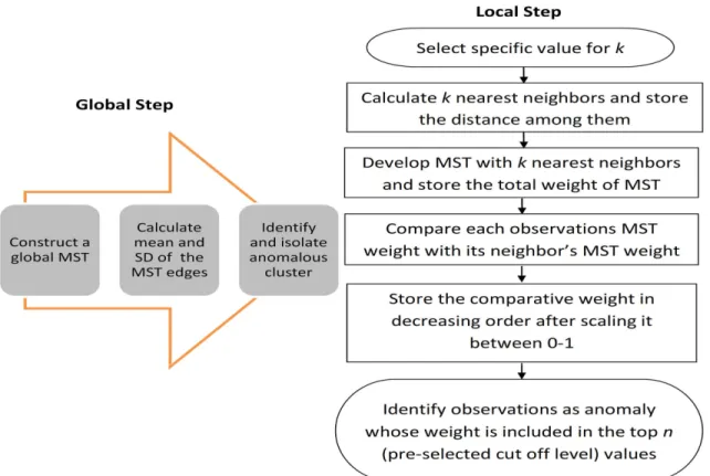
LIST OF FIGURES
FIGURE Page
1.1 Types of anomalies. (Reprinted from [1]) . . . 2
1.2 Shortcoming of Euclidean distance in a data space embedding complicated struc-tures and a possible solution. . . 6
1.3 Formation of an MST: the left panel is the initial graph. In the right panel, the dark black edges form the minimum spanning tree. The total MST weight is109. . . 7
1.4 Major categorizations of anomaly detection methods. . . 9
2.1 Anomaly detection using the proposed framework . . . 23
2.2 Flowchart of the proposed method. . . 28
2.3 Select the range ofkvalues. . . 29
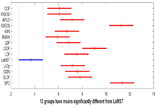
2.4 Post hoc analysis on the ranking data obtained by the Friedman test. This analysis is under the practicalksetting. . . 34
2.5 Anomaly detection in a streaming batch . . . 44
2.6 Decision tree based on the anomalies identified by LoMST method. . . 48
3.1 Post hoc analysis on the ranking data obtained by the Friedman test. . . 72
4.1 Autoencoder framework using feed-forward neural networks. Blue circles repre-sent nodes/neurons and dotted lines reprerepre-sent neuron connections. . . 79
4.2 MST regularized autoencoder can maintain the structural similarity in low dimen-sional representation.. . . 94
LIST OF TABLES
TABLE Page
1.1 Public benchmark datasets used in the performance evaluation study. . . 17
2.1 qselection policy for theArrhythmiadata set . . . 24
2.2 Performance comparison based on the bestk value . . . 31
2.3 Performance comparison based on the practicalkchosen according to our selection policy . . . 31
2.4 Number of true positive detections of the 14 methods in the bestksetting . . . 32
2.5 Performance comparison based on bestkvalue for alternative neighborhood com-parison statistic . . . 32
2.6 Performance comparison based on ourkselection policy for alternative neighbor-hood comparison statistic . . . 33
2.7 P-values of pairwise comparison of LoMST method with the competing methods. . . . 35
2.8 Performance of the LoMST method. . . 36
2.9 Summary of the top 100 anomalies returned by the four approaches. . . 46
2.10 Most anomaly prone days according to the four methods. . . 47
3.1 Parameter values and settings used for NS-NMF, GNMF and SNMF. . . 70
3.2 Performance comparison among the NMF approaches. . . 71
3.3 The p-values of pairwise comparisons between the NS-NMF method with each of the three competing methods. . . 73
3.4 Number of true positive detections of the competing NMF methods. Bold entries represent the best detection performance in a respective dataset. . . 74
3.5 Summary of the top 100 anomalies. . . 75
3.6 Most anomaly prone days identified by the three methods. . . 77
4.1 Strategy adopted regarding parameters and components of the graph regularized framework. . . 91
4.2 Summary of autoencoder models. Here (X) indicates the model includes the criteria. 93 4.3 Performance comparison of the autoencoder approaches. . . 95 4.4 Number of true positive detections of the competing autoencoder methods. Bold
entries represent the best detection performance in a respective dataset.. . . 97 4.5 Comparison between reconstruction loss based detection and those using an
exist-ing anomaly detection methods after the MST-regularizer. . . 98 4.6 Change in detection outcomes using the new denoising approach under the MDS
formulation. . . 99 4.7 Performance of GAN-based anomaly detection with and without the MST regularizer.100
1. INTRODUCTION AND LITERATURE REVIEW
1.1 Anomaly detection: An overview
Anomalies, also referred to as outliers, are loosely defined as data points or a cluster of data points which lie away from the neighboring points or clusters and are inconsistent with the overall pattern of the data. It is difficult to come up with a universal definition of anomalies as it often depends on the context.
Anomalies could be categorized into many different types [1, 2]. They can be global and distant from the majority of data points or can belocaland homogeneously mixed with the regular data points unless properly separated. In Fig. 1.1, pointA1 and A2 are referred to as the global point anomalies as they are far away from all of the existing clusters (C1, C2, and C3) and data points. PointA3 is referred to as a local point anomaly. At first look, it seems like a legitimate point as it lies close to the points in data cluster C1. But, if we magnify the local neighborhood and compare its position only with respect to the points from cluster C1, pointA3 becomes more visible as an anomaly. Anomalies can also form a cluster. In Fig. 1.1, for example, we can identify clusterC3as an anomalous cluster as it is different from the other clusters in size.
There are three broad categories of anomaly detection approaches, depending on the labels of the data in a training set. Supervised anomaly detection comes into play when we have appropri-ately labeled training data in advance (both normal and abnormal) so that we can train a model based on these labeled data and use it to decide the labels of future data. Support Vector Machine (SVM) [3] or Artificial Neural Network (ANN) [4] are the examples of this approach. But, when we have only normal instances and no anomalous data, we can still use the normal data to train a model and classify future observations as anomalies if they deviate from the normalcy. This normal-data-only approach is known assemi-supervised anomaly detection. One-class SVM [5]
Figure 1.1:Types of anomalies. (Reprinted from [1])
falls under this category. The most difficult scenario is the absence of any label of the data. As a result, it is not possible to conduct a supervised training. One, therefore, has to rely entirely on the structure of the dataset and detect the anomalies, if any, in an unsupervised manner. This last category is known asunsupervised anomaly detection. Throughout this dissertation, we are going to work with anomaly detection problems falling into this latest category.
1.2 Motivation
Anomaly detection problem arises in many real-life applications including but not limited to credit card fraud detection, cybersecurity, medical image analysis, surveillance, and industrial process safety. In the current industrial setting, various multi-platform devices, sensors converge into one centralized, interconnected network and lead to the burst in the availability of unlabeled stream-ing data points. As a natural consequence, it creates the need for developstream-ing suitable analytic techniques to analyze these high dimensional data stream in an unsupervised fashion and detect unusual, anomalous behaviors in real-time.
To detect anomalies, using unlabeled data streams pushes us to the territory of unsupervised learning. Consider the example of a hydropower plant which works as a motivation behind this dissertation. It operates with turbine systems that are instrumented with dozens of sensors. Each turbine has subcomponents or functional areas such as several bearing systems, a generator, etc. Sensors collect various types of data in real-time such as the temperature of oil inside the bearing systems, vibrations in each functional area, a variety of harmonics in functional areas, and many more. In total, each turbine collects more than 200 attributes from its sensors. The sensor data is then stored in a central control system and kept as time stamped historical data points. Anomaly can be triggered from various sources and can cause a range of problems.
When a service/maintenance engineer suspects that there is a malfunction in a turbine, she/he extracts a dataset from the control system that contains the collected sensor data for that turbine for the selected period of time (few weeks to few months), and then stores this data in a rela-tional database or simply in a .csv file for further analysis. Staring at a spreadsheet of data, a service/maintenance engineer often wonders if there is an automated, efficient way to distinguish the anomalies in the turbines. This problem falls under unsupervised anomaly detection because the historical dataset in the spreadsheet almost surely has both normal data and anomalies. It is just that the service/maintenance engineers do not know which is what. What makes this problem
more challenging is the number of attributes in the data space, amounting to a few hundreds and making a low-dimensional visualization difficult to carry out. An efficient offline anomaly detec-tion approach can surely help a lot but still not enough to identify anomalies as they appear which is vital to protect the health of components. Equally important is to look at the streaming nature of the data. As data streams arrive in real-time for analysis, examining them one by one manually is not a practical approach. A pressing need is to have an automatic detection technique that could provide a list of potential anomalies by evaluating the stored high dimensional data points in small batches.
1.3 Problem with embedded manifold and a new solution
Now, as we have already laid out the motivation behind our work by illustrating the practical industrial need, let us move into the technical challenges of an unsupervised anomaly detection approach that we need to solve.
A fundamental issue in any anomaly detection approach is deciding on the similarity metric which will be used to distinguish the anomalous observations from the normal ones. Though a variety of approaches have been proposed in all these years, the vast majority of them rely on the Euclidean distance and some of its statistical variants. The concept is pretty straightforward: if
||A −B||2 > ||A −C||2, it implies that A and C are more similar. When a minority of data points are dissimilar from a majority of data points, then the minority of data points are considered anomalies. However, in high dimensional spaces, pairwise Euclidean distances become similar and as a result Euclidean distance-based discriminative methods may not be able to differentiate among the relative position of data points accurately [6].
In a higher dimensional space, data points are also more likely to embed a complicated struc-ture thus leading to a nonlinear manifold. A manifold is a topological space that locally resembles Euclidean space near each point but globally it may not. In the presence of such a complicated space structure, the direct Euclidean distance between two points does not represent their intrinsic
distance as it may no longer be possible to reach directly from one point to another point through a straight line. The later problem is more severe as it can occur even in a low dimension and we want to treat this issue first.
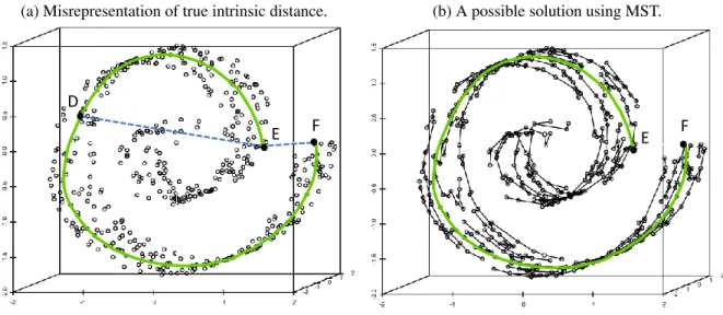
Let us elaborate on the problem of a structured data space and the embedded manifold through an example illustrated in Fig. 1.2. This example is inspired by the work of [7]. When the data forms a nonlinear structure in space, the distance measure between two data points on this structure is then constrained by such structure and should be accordingly construed. Consider the data points E, D, F in Fig. 1.2(a). With the structure, E-to-D is closer than E-to-F, meaning that E and D are more similar to each other than E and F. But if using the Euclidean distance, represented by the dotted lines, EF is shorter than ED, making the learning algorithm to believe E and F more similar to each other than E and D. Note that this example happens in a 3 dimensional space. It means that when the space structure exists, the Euclidean distance can break down even in a relatively low-dimensional space and lead us to the wrong conclusion. A similar real-life example illustrating a structured space is the flight route selection between two places on the earth’s surface. It is not the direct Euclidean distance that governs the route selection, but the distance constrained by earth shape; this space-constrained distance is known as geodesic distance. In Fig. 1.2(a), the solid green line highlights a geodesic path between E and F.
As it is arguably more difficult to ascertain a priori whether a data space embeds a structure, we think it is safe to assume the presence of a structured space. This assumption raises a related ques-tion concerning the computaques-tion of the true intrinsic distance among data points without knowing the shape of the structure beforehand. In this dissertation, we devise a new similarity measure based on the concept of the minimum spanning tree (MST). What motivates us to choose MST as a similarity measure is the fact that as the number of data instances increases, the shortest path distances among data instances provide a good approximation to the geodesic distances.
Before going into further details, let us first look how this MST based similarity concept works. Suppose that one has a connected edge weighted undirected graphG = (V, E), whereV denotes
(a) Misrepresentation of true intrinsic distance.
E F D
(b) A possible solution using MST.
E F
Figure 1.2:Shortcoming of Euclidean distance in a data space embedding complicated structures and a possible solution.
the collection of vertices and E represents the collection of edges with a real valued weight eij assigned to each of them, where i, j represent a pair of vertices fromV. A minimum spanning tree is a subset of the edges inEof graphGthat connects all the vertices inV, without any cycles and, with the minimum possible total edge weight. In other words, it is a spanning tree whose sum of edge weights is as small as possible. Let us defineDij as the distance (Euclidean) between vertexiand vertexj connected by an edge. The weight, however, does not always mean physical distances. For example, the weight could represent the amount of flow between a pair of vertices or sometimes the cost of constructing this edge.
Consider a simple example in Fig. 1.3, left panel, where there are 10 vertices and 16 edges. Each of the edges has a unique edge length, which is represented by a numeric value. If we want to connect all the nodes using a subset of the given edges without forming a cycle, there could be many such combinations, but the one(s) having the minimum total edge length is the MST. MST may not be unique, but for this example, it is unique and shown in the right panel of Fig. 1.3. The edges in black color represent the selected nine edges from the 16 in total, forming the MST.
Figure 1.3:Formation of an MST: the left panel is the initial graph. In the right panel, the dark black edges
form the minimum spanning tree. The total MST weight is109.
provide a new measure of distance between the vertices. Although the distance between a pair of immediately connected nodes is still Euclidean, the distance between a general pair of nodes (i.e., data points) is not. Rather, it is the summation of many small-step, localized Euclidean distances hopping from one data point to another point. For example, the new distance between the two colored vertices is12 + 11 + 13 + 10 + 9 = 55 (right panel), while their original distance in the left panel is23. We store inMij the new pairwise distance of vertices in the MST for future use instead of the typical Euclidean distances, Dij . As the MST reflects the connectedness among data points in a nonlinear manifold, the MST-based distance is the geodesic distance between two data points, which, according to [7], provides a better metric to differentiate them.
MST [8, 9] has the capability of approximating the geodesic distance in the presence of non-linear manifold. To achieve that it only uses the knowledge of neighboring points, nothing more than that. MST can be applied to any dataset after the data points are represented by a graph object. We can do so by considering each observation as a vertex and the pairwise Euclidean dis-tances among the vertices as the edge weights. Please refer to Fig. 1.2(b), where MST track the
geodesic path to provide an approximation of geodesic distance between E and F. There are three major algorithms [10, 11, 12] that can construct an MST for a given graph. The computational cost of constructing an MST isO(nlogm), wheren is the number of edges in the graph andmis the number of vertices. Here,n is m2 in our applications (one edge for every pair of vertices, i.e., a fully connected graph), which suggest a time complexity of O(m2)in constructing an MST, and because of this, an MST can be constructed efficiently even for a large dataset.
1.4 Related works
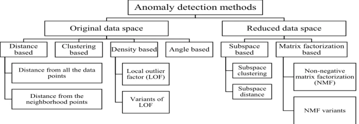
Anomaly detection methods in the literature can be categorized into some major domains depend-ing on the main theme of their detection mechanisms. The detection can be carried out both in the original data space and in a latent space or subspace. The number of variables in latent space or subspace is generally lower than the original data space. Whatever route we choose to follow, there are pros and cons associated with each of them which plays a significant role in the accuracy of the final detection outcomes. So, instead of grouping them based on their detection philosophy, we want to view the anomaly detection approaches from these two different perspectives as in our work we decide to contribute in both of these scenarios. For a more clear understanding of the flow of anomaly detection research, we summarize the major approaches accordingly in Fig. 1.4.
1.4.1 Anomaly detection in original data space
The commonality among the methods highlighted in this subsection is that they all detect anoma-lies using the original data points without transforming them into latent space or projecting into subspaces.
1.4.1.1 Distance-based methods
The first variant is the distance-based methods which consider a point as an anomaly if it lies further away from the majority of the data points [13]. The distance-based criterion entails a number of
Anomaly detection methods
Original data space
Distance based
Distance from all the data points
Distance from the neighborhood points
Clustering
based Density based
Local outlier factor (LOF)
Variants of LOF
Angle based
Reduced data space
Subspace based Subspace clustering Subspace distance Matrix factorization based Non-negative matrix factorization (NMF) NMF variants
Figure 1.4:Major categorizations of anomaly detection methods.
variants to handle the complexity in real life. For instance, thek-nearest neighbor (k-NN) based methods compare a candidate data point with itsknearest neighbors, rather than all the data points, because it was believed doing so enhances the detection capability [14, 15]. Anomaly scores are also defined as the ratio of the average of the distances from the test point to its k-NN’s and the average pairwise distance within thek-NN set [16]. One of the major downsides of these distance-based methods is: if the dataset has multiple clusters of varying density then they would not be able to separate local anomalies (i.e., anomalies only with respect to a single cluster) successfully.
1.4.1.2 Density-based methods
• Local outlier factor (LOF): The density-based approaches consider a point as an anomaly if the density around it is considerably lower than the density around its neighbors. The first of its kind and which is also by far the most popular method as well as the most cited work in the anomaly detection literature is known as local outlier factor (LOF) [17]. It is based on an idea calledlocal density which is estimated by the distance at which a point can be reached by its neighbors. By comparing the local density of an object to the local densities
of its neighbors, one can identify the anomalies. A drawback of this popular method is that it works pretty well in the presence of the spherical shaped cluster but fails to identify the irregular geometric shaped clusters especially when linearly correlated points form a cluster. Connectivity based anomaly factor (COF) [18] claimed to solve this problem by introducing a shortest path based chaining approach. The main argument behind COF is that ‘Low density does not always imply the anomalousness but the low connectivity to neighboring points surely does’. It differs from LOF by proposing a new incremental way of calculating the nearest neighbors.
• Variants of LOF: Due to the popularity of LOF method, variants of the LOF method was introduced within a short span of time to address the problems that could potentially limit the performance of the original LOF. Influenced outlierness (INFLO) [19] was proposed to compare the local density of an object to the average of its influence space. It is based on LOF, but it expands the neighborhood of the object to the influence space of the object and considers both the original neighborhood and the reverse neighborhood of an object. INFLO was introduced in order to handle the case where clusters with varying densities are in close proximity. Local density factor (LDF) [20] computes a kernel density estimation known as local density estimate (LDE), over a user-given number of k nearest neighbors. The LDF score is the comparison of LDE for an observation to its neighboring observations. Local outlier probabilities (LoOP) [21], was introduced which computes a local density based on the probabilistic set distance for observations, with a user given k nearest neighbors. The density is compared to the density of the respective nearest neighbors, resulting in the local outlier probability. The value ranges from 0 to 1, with 1 representing the greatest outlierness. The advantage of this probability based metric is that now anomaly scores are more interpretable and can be compared over datasets.
No matter what approach these methods adopt to calculate the local density, they all suffer from the problem of selecting a suitable value fork(number of nearest neighbors) like all otherk
-NN based models. As we are working in an unsupervised setting it would not be possible to apply method like cross-validation to estimate a suitablek. In the original paper introducing LOF, it was suggested to use a range of k values and then for each observation select thek value that results a maximum anomaly score. In the literature when comparing methods, it is a common practice to use either the bestk or the average result over a range of k values. However, in Section 2, we propose an adhoc policy for selecting the neighborhood sizek.
1.4.1.3 Clustering-based methods
The density-based methods provide a different perspective for identifying anomalies, which is to consider the data clustering tendency. There are clustering approaches which are specifically developed for anomaly detection. There are three categories of clustering-based anomaly detection algorithms. Methods in [22, 23] fall under the first category, which identifies instances that do not belong to any regular cluster as anomalies. The second group of clustering technique is a variation of the first group and uses a clustering algorithm to detect clusters and then calculate an anomaly score by taking the distance from a point to its nearest cluster center. Both of these groups do not take into account that anomalies can also form clusters and in those cases such methods will fail to detect these anomalous clusters. The third category of clustering based algorithms [24, 25] was introduced to tackle this problem which assumes that normal observations belong to large and dense clusters, whereas anomalous observations belong to small and sparse clusters or lie further away from the cluster centroid.
1.4.1.4 Angle-based methods
Angle-based methods were introduced with the consideration that angles are a more stable measure in high dimensions compared to distances [26]. One major limitation of this method is the high computational time it requires to calculate the angles.
but they are all similar in at least one aspect; which is the use of the Euclidean distance. We already argued that the use of Euclidean distance-based metric loses its effectiveness in a data space embedding inherent structures, which is most likely of high dimensionality. So, no matter what method we select to modify and develop further or even propose a new method, as long as we are using the Euclidean distance, we cannot capture the structure of the data and our detection would be wrong.
We believe that instead of making incremental improvements over any one of the existing methods, we need to rethink this fundamental issue of how we differentiate data instances in unsu-pervised learning settings. The current reliance on Euclidean distances appears to run out of steam. In Section 2, we develop a local MST (LoMST) based anomaly detection approach, capable of de-tecting anomalies by comparing the connectivity of each point to its neighbors.
1.4.2 Anomaly detection in reduced data space
As more and more high dimensional data comes into play, people start to realize the curse of dimensionality and how it reduces the effectiveness of the Euclidean metric. Consequently, the research effort in anomaly detection shifted towards evaluating data points in reduced dimensional space.
1.4.2.1 Subspace based methods
The key argument in favor of subspace based methods is that not all variables are relevant for discovering anomalies and it would be wiser to consider relevant subspaces rather than considering the entire feature set. One could devise different strategies in selecting the subspaces. For instance, principal components analysis (PCA) [27] renders the subspace that has the largest variances most relevant, while multidimensional scaling (MDS) [28] selects the subspace that preserves the interpoint distances in their low dimensional representation. They are both capable of preserving the original data space structure in linear vector spaces, but they tend to lose the data structure in
the presence of nonlinear manifolds [7].
A grid-based subspace clustering [29] was proposed for searching sparse, rather than dense, grid cells to report objects contained within those sparse grid cells as anomalies. High-dimensional outlying space (HOS) miner [30] ranks a point as an anomaly in any subspace if the sum of its distance from its k-nearest neighbors crosses a predetermined threshold. Subspace clustering [31] can be also helpful as anomalies are found in abnormally few clusters or low dimensional clusters. Subspace outlying degree (SOD) [32] detects an anomaly based on its deviation to the subspace spanned by a set of reference points. The subspace is formed with those features where the reference points vary very little. But the success of this method depends on the tuning of neighborhood parameters just like thek-NN method. HicS (High contrast Subspaces) [33] relies on finding those subspaces where attributes are correlated (statistically dependent). GLOSS [34] suggested that global neighborhoods should be considered when detecting anomalies locally in selected subspaces.
Subspace methods undoubtedly made progress in the unsupervised anomaly detection litera-ture. But fundamentally, finding out the right subspaces to explore and how to compare anomalies from different subspaces are still a difficult problem to solve. However, autoencoder [35, 36, 37] came out as a rescue to solve the problem of finding a proper low dimensional subspace. It does so by reconstructing the data again from the subspace by minimizing the difference between re-constructed and original data. So, now, the reduced data space coordinates can be utilized for unsupervised learning. But, again, it suffers from the problem of embedded manifold due to the use of Euclidean distance-based similarity measure. Therefore, in Section 4, we propose a new graph regularized autoencoder which can overcome the problem of a complicated manifold and thereby generate a low dimensional representation useful for anomaly detection.
1.4.2.2 Matrix factorization based methods
• NMF for anomaly detection: Matrix factorization based methods have been applied suc-cessfully for a long time to represent the data in a reduced dimensional space for better learning and hence achieve the clustering benefits. These methods essentially factorize the original data matrix into two low rank matrices. One helps us to obtain the mapping of orig-inal data points to latent space and another depicts how the latent space is created from the original attributes. These low rank matrices help us to obtain clustering assignments and the attribute distribution of the clusters. However, these approaches have not gained sufficient popularity in the anomaly detection community. This may be due to the fact that traditional matrix factorization like the principal component analysis (PCA) produces low rank matrices consisting of negative values and positive and negative weights, which tend to cancel each other in reconstructing the original matrix and hence provide no intuitive meaning, while on the other hand, one would like to know the ‘meaningful’ attribute distribution of these clusters for anomaly detection, so as to evaluate the suspicious observations against them. For this reason, the nonnegative matrix factorization [38, NMF] method, which imposes the non-negativity constraint in matrix factorization and only allows additive linear com-binations of components, comes across as a better candidate for the purpose of anomaly detection. NMF has the capability of generating both clustering assignments and meaning-ful attribute distribution in two separate matrices. Immediately after its introduction, NMF not only becomes a powerful tool for clustering [39], but it also shows enough potential as an anomaly detection approach [40, 41]. In the presence of complicated manifolds, however, researchers notice that NMF starts to lose its efficiency [42, 43] as it only tries to approxi-mate the data without trying to mimic the similarity among observations in the latent space. In other words, the shortcoming of the original NMF in anomaly detection is attributed to that it has no provision to include the neighborhood structure information during the calcu-lation of the factored matrices. So, we once again revisit the fundamental problem related to
capturing the inherent structure of the dataset.
• Variants of NMF: Two recent versions of NMF tried to tackle this problem. One of them is the graph regularized NMF [43, GNMF], which regularizes the original NMF formulation using a Laplacian matrix. But GNMF still constructs the neighborhood similarity matrix based on simple Euclidean distances. The second NMF variant is the symmetric NMF [42, SNMF], which uses only the similarity information while excluding the attribute informa-tion to generate the low rank matrices. In the absence of the attribute informainforma-tion, SNMF depends on a dense pairwise similarity measure which leads to a computational disadvan-tage. Also, by abandoning the original attribute information in its formulation, SNMF makes its detection outcomes less interpretable or ‘meaningful’ than NMF or GNMF. So, capturing and preserving the neighborhood structure in a computationally efficient way for meaningful anomaly detection in latent space is still an open problem to solve.
In Section 3, we propose a new neighborhood structure assisted NMF formulation for anomaly detection which takes into account the importance of neighborhood connectivity into account dur-ing factorization. To capture the neighborhood similarity, we make use of MST instead of the Euclidean distance-based similarity and thereby attain the advantage of geodesic similarity.
1.5 Performance metric
To evaluate the performance of the competing approaches in benchmark datasets, we use a pre-cision at N[44, P@N] criteria. This is a widely used performance metric in anomaly detection. When observations are sorted in descending order according to their anomaly scores, the P@N identifies the proportion of the correct anomalies in the top N ranks. In the circumstance where the true number of anomalies, |O| is known, like in the benchmark datasets to be described in Section 1.6, we use that value as our choice ofN and treat it as the same cut-off for all methods in comparison. When N is the number of true anomalies, the number of false alarms is implied once P@N is calculated, which is N −N ×P@N. That is why we only present P@N in the
benchmark studies. In reality, when the number of true anomalies is not known, the main objective in anomaly detection is still to increase P@N for a fixedN, i.e., to have a higher detection rate within the cut-off threshold.
For a datasetDB of sizem, consisting of anomaly setO ⊂DBand normal datasetsI⊆DB, such thatDB =O ∪I,P@N can be formulated as
P@N = #{o ∈O|rank(o)≤N}
N , where N =|O|. (1.1)
WhenN is unknown in practical settings, a good practice is to chooseN larger than the esti-mated number of anomalies but small enough so that it makes follow up identification operations feasible. The rationale behind this choice lies in the fact that the false positive rate for anomaly detection problems is generally high, especially compared to the standard used for supervised learning methods. Despite a relatively high proportion of false positives, anomaly detection meth-ods can still be useful, particularly used as a pre-screening tool. By narrowing down the candidate anomalies, it helps human experts a great deal to follow up with each circumstance and decide how to take proper action or deploy a countermeasure.
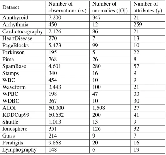
1.6 Benchmark datasets
In this study, we use 20 benchmark anomaly detection datasets from [44] for the purpose of per-formance comparison. In Table 1.1, we summarize the basic characteristics of these 20 datasets. For all of these benchmark datasets, we know the total number of anomalies and the label of the individual observation, i.e., whether it is an anomaly or not. There are several versions of these datasets available depending on the data cleaning and preprocessing steps involved. For our anal-ysis, we choose to use the normalized version of the datasets with all missing values removed and categorical variables converted into a numerical format.
Table 1.1: Public benchmark datasets used in the performance evaluation study.
Dataset Number of Number of Number of
observations (m) anomalies (|O|) attributes (p)
Annthyroid 7,200 347 21 Arrhythmia 450 12 259 Cardiotocography 2,126 86 21 HeartDisease 270 7 13 PageBlocks 5,473 99 10 Parkinson 195 5 22 Pima 768 26 8 SpamBase 4,601 280 57 Stamps 340 16 9 WBC 454 10 9 Waveform 3,443 100 21 WPBC 198 47 33 WDBC 367 10 30 ALOI 50,000 1,508 27 KDDCup99 60,632 200 41 Shuttle 1,013 13 9 Ionosphere 351 126 32 Glass 214 9 7 Pendigits 9,868 20 16 Lymphography 148 6 19 1.7 Hydropower dataset
Apart from the public benchmark datasets, a real-life dataset generated from a hydropower plant is also used in the performance comparison study. The hydropower data that was initially received was time-stamped (a total of seven months worth of data) and divided into different functional areas (turbines, generators, bearings etc.). The data was collected at 10-minute interval each day. But it was not always continuous and some days from each of these seven months were missing. After combining all data across all functional areas, there are 9,508 observations (rows in a data table) and 222 attribute variables (columns in a data table). Each row has a time stamp assigned to it. Attribute variables are primarily temperatures, vibrations, pressure, harmonic values, active power etc.
We conducted some basic preprocessing and statistical analysis [45] in order to clean the data. To maintain the similarity with the 20 benchmark datasets, we normalized the data, removed the duplicate rows as well as the rows with missing values. Additionally, we also did correlation analysis and plotted histogram, density and box plots. The data preprocessing did yield a small number of data records that are so far off from other data records. When confirming with the domain expert who provided the data, it was confirmed that those records were due to a recording mistake. After removing them, the total number of observations comes down to 9,219.
Here, different from the benchmark datasets, we no longer have the information of the number of true anomalies. After consulting the operating manager who provided this dataset, we are ad-vised to report top 100 anomalous time stamps to the manager. The manager would follow up and check the status of the operation in detail, for instance, by manually examining operational logs and physical conditions of components, and then confirm us about the validity of the findings.
1.8 Organization of this dissertation
The dissertation proposes three unsupervised anomaly detection algorithms all revolving around our newly developed MST based dissimilarity metric to capture the geodesic similarity among observations. These algorithms have the potential to tackle the problem of high dimensional data with manifold embedding property better than the simple Euclidean distance. In addition, the dissertation also proposes the online version of these algorithms to handle the streaming data and enable real-time detections. All of these algorithms are tested on 20 public benchmark datasets and the real-life hydropower dataset to prove their worth.
The rest of the dissertation is organized as following. Section 2 develops a local MST (LoMST) based anomaly detection algorithm which detects both local and global anomalies by adopting a two step procedure. When compared with a wide variety of neighborhood based anomaly de-tection algorithms, it achieves superior and significantly better dede-tection capability. Section 3 develops a neighborhood structure assisted NMF (NS-NMF) method to prove the fact that
neigh-borhood structure can essentially help the matrix factorization principles to achieve better anomaly detection capability and MST based similarity measure is an ideal candidate for such neighbor-hood approximation. It proposes a new NMF formulation by providing a detailed theoretical and empirical comparisons with some of the existing state of art formulations. Section 4 argues for the necessity of dimensionality reduction before applying any anomaly detection algorithm and the importance of autoencoder mechanism to do it in an unsupervised way. Then a graph regularized autoencoder is developed to deal with the nonlinear embedding problem which can be extended into today’s powerful deep learning frameworks and thus applicable to data of any size and type. Finally, Section 5 summarizes the key contributions and highlights potential extensions beyond this dissertation.
2. LOMST: A LOCAL MST BASED ANOMALY DETECTION APPROACH AND ITS APPLICATIONTOHYDROPOWERTURBINES*
In this chapter, we use the concept of MST on a local neighborhood level and develop a local MST (LoMST) based anomaly detection method. The merit of this method is that it provides a new distance measure among the observations in the local neighborhood which is capable of capturing the relative connectednessof data points/clusters in a complicatedmanifold. We also proposeastrategytodetectglobalanomaliesas apreprocessingstepbeforedetectinglocalpoint anomalies. The proposed method is compared with 13 popular anomaly detection methods on 20 benchmark datasets, demonstrating a considerable improvement in its ability of identifying anomalies. Furthermore,itisalsoappliedtothedatasetgeneratedfromahydropowerturbineand demonstratesremarkabledetectioncompetence.
2.1 Introduction
Ourproblemismotivatedbytheanomalydetectionproblemencounteredinahydropower gener-ationplantasdiscussedinSection1.7. Theproblemdemandsforananomalydetectionapproach thatcandealwithhighdimensionaldatainastreamingfashion. Itwasarguedin[7]thatthehigher adataspace’sdimension,themorelikelyitembedsaninherentstructureforminganonlinear man-ifold. As a result, geodesic distance mustbe used instead ofEuclidean distances ina nonlinear manifoldtoreflectaccuratelythedistancebetweendatapoints.Wewanttonotethatacomplicated structurecouldhappentolowdimensionalspaces,too,sothattheEuclidean-baseddistancemetric couldlose itseffectivenessin lowdimensionalspacesas well. Empirically,however, people
ob-*Reprintedwithpermissionfrom“UnsupervisedAnomalyDetectionBasedonMinimumSpanningTree Approx-imatedDistanceMeasuresanditsApplicationtoHydropowerTurbines”byImtiazAhmed,2019.IEEETransactions onAutomationScienceandEngineering,16(2),654-667,Copyright2019byIEEE.
*Reprinted withpermissionfrom “O-LoMST:AnOnlineAnomalyDetectionApproach AndItsApplicationIn AHydropowerGenerationPlant”byImtiazAhmed,2019.2019IEEE15thInternationalConferenceonAutomation ScienceandEngineering(CASE),762-767,Copyright2019byIEEE.
serve such instances happening more often in higher dimensional spaces and tend to associate the loss of effectiveness in Euclidean measures with the high dimensionality [46].
Geodesic distance is the minimum possible distance between two points in a curved surface like the surface of the earth. It was also shown [7] that as the number of data instances increases, the shortest path distances among data instances provide the best approximation to the geodesic distances. Driven by this insight, what we propose here is to use a minimum spanning tree (MST) to provide an approximation of geodesic distances in a structured space and then use it as the (dis)similarity metric. More specifically, we model the data observations as a network of nodes where edges represent the Euclidean distance from one another. An anomalous node would be the one which is less connected to its neighboring nodes. An MST is a measure that can capture the relative connectedness among nodes, while at the same time, approximates the geodesic dissimilar-ities among observations forming a nonlinear manifold. It has been shown in the literature [47, 9, 8] that MST is indeed a capable approximation of geodesic distances in a high dimensional data space embedding complicated structures.
There are several positive aspects associated with the proposed approach. First, the distance between any two nodes in an MST is no longer the direct Euclidean distance between them; rather it is the new dissimilarity metric which takes into account the overall connectivity among data points reflecting the complexity in a structured data space. So, the MST-based dissimilarity measure is a good candidate to approximate the geodesic distance and has the potential to overcome the limitation of direct Euclidean distance under such circumstances. Next, to take into account the presence of clusters of different shapes and densities, we develop MST locally and compare a node’s connectedness with its neighboring cluster only. Doing so enhances the detection ability of the local, point-wise anomalies.
We are aware that MST has been used to find anomalies [48, 49, 50, 51, 52]. The objective of most of them [48, 49, 50, 52] is to isolate the clustered anomalies by removing the links of the global MST one by one. Our attention in this chapter is more about local, point-wise anomalies.
What was done in [48, 49, 50, 52] is similar to Stage 1 of the proposed method (more details later), which is really a preprocessing step in our method. Our main attention is on Stage 2, the local anomaly detection. The concept of [51], is a bit different as the author proposed to label any new test observation as an anomaly by comparing them to the most concentrated subset of points in the training sample. To find out the most concentrated subsets the author chooses to apply the k-point MST. So, this approach is applicable for semi supervised anomaly detection/novelty detection scenario where we know beforehand that the training sample is free from anomalies and can utilize it to detect any abnormality in the test sample. This is fundamentally different from the unsupervised problem we are dealing with. In our case we do not have any information about the label of the training data. Apart from that our approach utilizes neighborhood-based local MST which is entirely different from the concept of k-point MST.
The rest of the chapter unfolds as follows: Section 2.2 describes the main idea of our pro-posed approach and the steps of the algorithm developed. Section 2.3 presents the comparative performance of our method with respect to other prevalent methods on 20 benchmark datasets. Section 2.4 describes the online version of the LoMST approach for streaming data. Section 2.5 analyzes the performance of the offline and online algorithms in hydropower dataset. Finally, we conclude the chapter in Section 2.6.
2.2 MST-based anomaly detection method
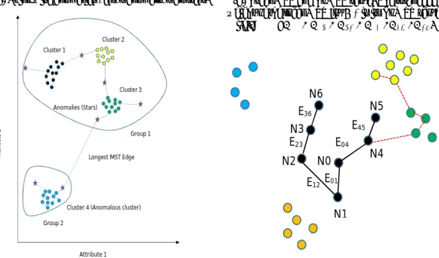
As mentioned earlier, our main focus is to come up with a minimum spanning tree-based distance metric which reflects the dissimilarity among anomalies and normal data points in structured data spaces. Please refer to 1.3 for a brief discussion of the MST’s role in manifold approximation. Using MST helps address another complexity often encountered in anomaly detection, which is to detect pointwise anomalies in the presence of anomalous clusters. Fig. 2.1(a) presents an illus-trating example in which there are well separated four clusters whose structures are not difficult to identify. The star shaped symbols represent the local anomalies relative to their nearest cluster.
Cluster 4 itself is an anomalous cluster whereas cluster 1, 2 and 3 are regular clusters. Existing anomaly detection methods such as LOF [17] adjust their view field on anomalies by setting differ-entk’s, the value of the nearest neighbors: when a smallkis used, the local anomalies are detected but the anomalous cluster 4 will be unidentified, while when a largekis used, all the instances can be separated into two parts, namely, Group 1 and Group 2, in which Group 2 contains cluster 4. Under that circumstance, one has to pay the price of not detecting the local anomalies in Group 1. The reason that using MST can help is because MST can be used as a clustering tool [50, 48] to isolate the anomalous clusters first. Then, it can be refined to define the dissimilarity distances in a local setting. This thought points to a two-stage procedure, which is to remove the global anomalous clusters first and then detect the local point-wise anomalies later; both stages use MST as the common methodological foundation.
(a) Point-wise anomalies versus anomalous clusters.
Cluster 1
Cluster 2
Cluster 3
Cluster 4 (Anomalous cluster) Anomalies (Stars) Longest MST Edge Attribute 1 At tr ib ut e 2 Group 1 Group 2
(b) Local MST and LoMST score. The total edge weight of the local MST forN0is its LoMST score,
i.e.,WN0=E01+E12+E23+E04+E45+E36. N1 N0 N5 N3 N6 N4 N2 E12 E23 E36 E01 E04 E45
Figure 2.1: Anomaly detection using the proposed framework
anomalous clusters if they exist. The procedure is similar to the existing work of how MST is used [48, 49, 50]. First, we build a global MST using all the data points. The specific MST construction algorithm we use is in [10]. The reason we choose the algorithm in [10] is because it handles dense graphs well, while the other two algorithms [11, 12] handle sparse graphs better. And our case is a dense graph.
After the formation of the global MST, we then look for a long edge and treat it as the connect-ing edge between the anomalous cluster and the rest of the MST. Once this edge is disconnected, it separates the MST into two groups, and the smaller group is considered an anomalous cluster. One of the problems of deleting such edges is, in the absence of distant anomalies, normal points could be isolated and tagged as anomalies instead. So, we have to create a lower bound so that we can only delete the longest edge that crosses the bound. We decide to useµ+q*σ as the threshold whereµrepresents the average of the edge weight andσrepresents their standard deviation. Now, the choice ofqentirely depends on the data set and the distribution of anomalies. If we use a high q, then there will be no candidate edges to be deleted, on the other hand, too small aqwill lead to a large chunk of points detected as anomalies. As we are not sure about the structure of the data set beforehand, it is not easy to specify the best value forq. In our case, we evaluate several candidate qvalues from 2-5 and we found thatq=3 works reasonably well for most of the data sets.
This edge deletion procedure will be then iterated on the larger remaining group and see if there is another, less dominating anomalous cluster, until there is no anomalous long edge detected. This procedure is equivalent to a Phase I analysis in statistical quality control [53]. We have summarized theqselection policy for theArrhythmiadata set in Table 2.1 as an example.
Table 2.1: qselection policy for theArrhythmiadata set
Possible options Number of iterations required Number of true anomalies detected Number of false detection
Mean + 3SD (q=3) 2 3 2
Mean + 4SD (q=4) 1 0 0
Once the clustering decomposition stops in the first stage, then we move on to the second stage of identifying pointwise anomalies which is also the main contribution of our work. In the second stage, we go into the neighborhood level for each data point to determine its possibility as an anomaly. The neighborhood is determined by the number of nearest neighbors and parameterized byk. We will come back later to discuss the procedure of selecting the value ofk but for now let us assume we have a predetermined value fork.
Denote by R the rest of the data points after the anomalous clusters are removed in Stage 1. For any given data point inR, first, isolate itsk nearest neighbors and treat them as this data point’s neighborhood. Then, build an MST in this neighborhood. Considering the nature of these neighborhood MSTs, they are referred to as local MSTs (LoMST). The total edge length of the LoMST associated with the original data point is called the LoMST score for this data point and is considered the metric measuring its connectedness with the rest of the points in the neighborhood as well as how far away it is from its neighbors. For this reason, the LoMST is used as the differentiating metric to signal the possibility that the said data point may be an anomaly.
Consider the illustrating example in Fig. 2.1(b). Suppose that we have chosenk = 6and start with data pointN0. Then, we can locate its neighbors asN1,N2,N3,N4,N5andN6. The MST construction algorithm connectsN0to its neighbors in the way as shown in Fig. 2.1(b). ForN0, the total edge weight is WN0 =E01 + E12 + E23+ E04 +E45 +E36, which is deemed the LoMST score forN0. This procedure will be repeated for other data points and Fig. 2.1(b) shows another MST, which is forN5in the dotted edges.
The LoMST score for a selected observation will be compared with its neighbor’s score. Com-parison can be done in two ways. We can either compareW with the mean of the neighbor’s scores or with the mean-to-standard deviation ratio of the neighbor’s scores. Our analysis suggests that both comparison approaches have their own advantages depending on the structure of the dataset. When there are numerous anomalies, almost forming an anomalous cluster within a neighbor-hood, it would be better to use the mean-to-standard deviation ratio, as the mean of the neighbor’s
LoMST scores are severely contaminated by other anomalies. But when the anomalies are very few, point-wise scattered around, the mean of the LoMST score works just fine. Considering that we have the first stage to remove some of the anomalous clusters, in this second stage, we then use the mean comparison of LoMST scores as our default approach.
The step of comparison will be repeated|R|times covering all the nodes inR. Then the com-parison score will be scaled between 0 and 1 using the maximum and minimum value of the scores. From now on, we call the normalized scores as the LoMST scores. After that, these LoMST scores will be sorted in a decreasing sequence, where a greater score implies a higher possibility to be an anomaly. To compile a complete list of anomalies, we follow theP@N approach as described in Section 1.6, which is to select a prescribed cut off valueN and flag the topN instances on our tank list as anomalies. One main reason behind such a detection procedure is that unsupervised detec-tion methods tend to have a lower detecdetec-tion capability and higher false alarm rate, as compared to general supervised learning algorithms. As a result, unsupervised detection methods are typically used as a screening tool, flagging potential anomalies to be further analyzed by either a human operator or some more expensive procedure. A cut-off is therefore used to ensure the subsequent, more expensive or time consuming step practical and feasible.
For better technical understanding, the algorithm steps are summarized below. In addition, a flowchart of the proposed method separated into two stages is also highlighted in Fig. 2.2.
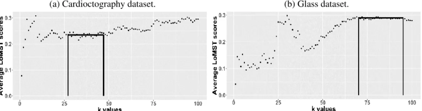
Now, to select an appropriate value for k, we adopt an approach based on the following ob-servations, illustrated in Fig. 2.3. When we plot the average LoMST scores for a broad range of k (here 1-100), we observe that at small k values, the average LoMST score tends to fluctuate, but as we keep increasingk, the average LoMST score will become stable at a certain point. Our understanding is that when a properkis chosen, the structure of the data is revealed and the label of the instances will become almost fixed, thus reflected in a less fluctuating LoMST score. If one keeps increasingk, there is the possibility that the data structure becomes mismatch with the as-signed number of clusters and the current assignments of anomalies and normal instances become
ALGORITHM 1:LoMST algorithm for anomaly detection
Input :Dataset (rows represent observations and columns represent attributes), number of nearest neighbors,kand cut-off level for identifying anomalies,N.
Output:Anomaly index set,T O
1 Develop set of verticesV, where each vertex represent a separate observation from the dataset;
2 Construct edges by calculating Euclidean distance between each pair of vertices and store them in
E;
3 Construct a global MST usingV andE, letSbe the set of edges of the resulting MST, whereS⊆
E;
4 Calculate the mean,µ, and the standard deviation,σof the edges inS; 5 InitializeR,O1,O2,T,N randLo=;
6 Calculate the longest edge fromSand store its length inLo;
7 ifLo≥µ+ 3σthen
8 Remove this edge from the MST tree formed by edges inS;
9 From the two disconnected trees, letA= {vertices contained in the smaller tree} andB=
{vertices contained in the larger tree};
10 SetS=B andO1=O1UA; 11 Go to step 6 ; 12 else 13 SetR=S; 14 Go to step 16 ; 15 end
16 foreach vertexri∈Rdo
17 Determine itsknearest neighbors and save them inN ri;
18 Construct a local MST using edges contained inEuv, whereu, v∈NiandEuv⊆E;
19 end
20 foreach vertexri∈Rdo
21 Calculate the total length ofri’s LoMST,Wri;
22 Calculate the mean (WN ri) of the total length of the LoMSTs associated with all vertices in
N ri;
23 Calculate the LoMST score forriasTi=Wri −WN ri;
24 end
25 Normalize the scores stored inT between 0 and 1 and rank them in decreasing order;
26 Identify the topN scores and store the corresponding observations as point anomalies inO2;
Figure 2.2:Flowchart of the proposed method.
destabilized again. Consequently, the average LoMST score could fluctuate once again. Based on this observation, our policy in choosingkis to select a range ofkwhere the average LoMST scores are stable. If there are more than one stable range, we will then select the first one. Here, for the Cardiotocographydataset, we can choose a k range from 27-47 and for theGlassdataset we can choose ak range from 70-95. Within the identified stable range, whichk to choose matters but matters less. What we suggest to select is thekvalue that returns the maximum standard deviation of the LoMST scores, because by maximizing the standard deviation among the LoMST scores, it increases the separation between the normal instances and anomaly instances and facilitates the detection mission.
(a) Cardioctography dataset. (b) Glass dataset.
Figure 2.3:Select the range ofkvalues.
2.3 Performance comparisons
In this section we wish to evaluate the performance of the MST-based method on a set of bench-mark testing datasets listed in Table 1.1 compared to an array of well established methods in the literature.
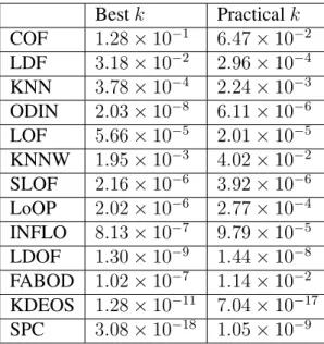
As our method is dependent on the parameterk, we mainly focus on the nearest neighborhood based approaches for a fair assessment. [44] provided detailed experimentation on 12 popular nearest neighborhood approaches based on the 20 aforementioned data sets. These 12 methods are Connectivity based Outlier Factor (COF), Local Density Factor (LDF), K-Nearest Neighbor (KNN), Outlier Detection using Indegree Number (ODIN), Local Outlier Factor (LOF), K-Nearest Neighbor Weight (KNNW), Simplified Local Outlier Factor (SLOF), Local Outlier Probabilities (LoOP), Influenced Outlierness (INFLO), Local Distance based Outlier Factor (LDOF) and Kernel Density Estimation Outlier Score (KDEOS). Traditional statistical process control (SPC) based approach could also be applied in the anomaly detection setting. We implemented one of the popular methods in SPC, the Hotelling T2 control chart [54]. We tested two versions while using the Hotelling T2 control chart: one with PCA that reduces the data dimension first and the other without PCA. It turned out that the T2 control chart without PCA performs slightly better than the PCA version. Hence, we only include the T2 result without PCA in the comparison tables to save space. In summary, we compare our MST-based approach with a total of 13 competing methods.
There is no guideline in the literature for how best to selectk. [44] simply tried a range ofk values (from 1 to 100) to obtain all the results and then choose the bestkvalue for each method. In the first comparison, we follow the same approach, labeled as the “bestk” comparison. The results are presented in Table 2.2. To better reflect the detection capability as they are compared to one another, we break down the comparative performance into four major categories, namely Better, Equal,CloseandWorse, as explained in the table. Please note that the “best”k value in Table 2.2 may be different for respective methods.
LoMST shows superior performance and clearly outperforms other methods. In 13 of the 20 data sets, LoMST either exhibits a uniquely best detection performance or is tied with some other methods to achieve the best detection capability. In only 2 data sets, LoMST performs in the worse category, meaning that its detection capability is 20% lower than the best alternative. If we rank each of the 14 methods in a scale of 1 to 14 according to its actual performance in relative to others, then the average rank for the LoMST method is 2.2, while some of the closest competitors areCOF(3.3),LDF(3.8),KNNW(4.5),KNN(5.0) andLOF(5.1).
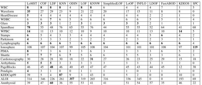
Understandably, the “bestk” is not practical, as in reality, people do not know the anomalies while selecting the bestk. Since we have come up with a strategy to select a practical value ofk, we use the samek value in the other 12 alternative methods that need thek (SPC does not need to knowk). The performance comparison based on the practicalk is presented in Table 2.3. We use the same performance breakdown as in Table 2.2. Our LoMST method continues to exhibit superior performance for being uniquely best in five of the 20 data sets and tieing other methods for achieving the best performance in another five data sets. The number of cases in the worse category is three. The average rank of the LoMST method is 2.8, slightly lower than that under the best k condition, while some of the closest competitors areCOF(4.2),KNNW(4.3),FBOD(4.9), KNN(5.3), andLDF(5.7). The mean ranks are included in the table, as the last row. Please find in Table 2.4 the number of true positive detections of 14 methods under the bestk setting, in which the best performance in every row is highlighted in boldface. To save space, we omit the same
Table 2.2:Performance comparison based on the bestkvalue `` ```` ```` ```` `` ```` ````
Performance (number of data sets)
Anomaly detection methods
LoMST COF LDF KNN ODIN LOF KNNW SimplifiedLOF LoOP INFLO LDOF FastABOD KDEOS SPC
Better (uniquely best result) 6 0 3 1 1 0 1 0 0 0 0 0 0 1 Equal (equal to the existing best result) 7 5 5 2 1 3 2 2 2 2 1 2 2 0 Close (within 20% of the existing best result) 5 10 6 7 8 8 7 6 6 5 7 5 1 1 Worse (not within 20% of the existing best result) 2 5 6 10 10 9 10 12 12 13 12 13 17 18 Mean relative rank 2.2 3.3 3.8 5.0 7.7 5.1 4.5 5.9 5.8 6.2 7.9 7.0 8.9 11.7
Table 2.3: Performance comparison based on the practicalk chosen according to our selection policy `` ```` ```` ```` `` ```` `
Performance (number of datasets) Anomaly detection methods
LoMST COF LDF KNN ODIN LOF KNNW SimplifiedLOF LoOP INFLO LDOF FastABOD KDEOS SPC
Better (uniquely best result) 5 2 1 1 2 0 0 0 0 0 0 2 0 1 Equal (achieving best result combinedly) 5 1 4 5 1 3 4 1 1 2 1 2 0 0 Close (within 20% of the best result) 7 11 4 6 8 7 9 8 7 7 6 6 3 3 Worse (not within 20% of the best result) 3 6 11 8 9 10 7 11 12 11 13 10 17 16 Mean Relative Rank 2.8 4.2 5.7 5.3 6.7 6.1 4.3 6.5 5.6 5.8 7.6 4.9 11.7 8.7
table under the practicalkas it conveys the same message.
In Section 2.2, we mentioned both the mean-based comparison statistic and the mean-to-standard deviation based comparison statistic. Tables 2.2 and 2.3 present the comparison results us-ing the mean-based statistic, which is our recommended default option. We also explore what if we use the mean-to-standard deviation ratio as the comparison statistic, and the results are presented in Ta
![Figure 1.1: Types of anomalies. (Reprinted from [1])](https://thumb-us.123doks.com/thumbv2/123dok_us/933844.2621070/15.918.194.734.182.642/figure-types-of-anomalies-reprinted-from.webp)