Abstract
The use of dynamic models and simulation environments in connection with software projects paved the way for tools that allow us to simulate the behaviour of the projects. The main advantage of a Software Project Simulator (SPS) is the possibility of experimenting with different decisions to be taken at no cost. In this paper, we present a new approach based on the combination of an SPS and Evolutionary Computation. The purpose is to provide accurate decision rules in order to help the project manager to take decisions at any time in the development. The SPS generates a database from the software project, which is provided as input to the evolutionary algorithm for producing the set of management rules. These rules will help the project manager to keep the project within the cost, quality and duration targets. The set of alternatives within the decision-making framework is therefore reduced to a quality set of decisions.q2001 Elsevier Science B.V. All rights reserved.
Keywords: Software development projects; Software Project Simulators (SPS); Machine learning; Evolutionary algorithms (EA)
1. Introduction
The use of dynamic models and simulation environments (Stella, Vensim, iThink, Powersim, etc.) in connection with software projects paved the way for tools that allow us to simulate the behaviour of such projects at the start of the 1990s. With these tools, which are named Software Project Simulators (SPS), the project manager could experiment with different management policies at no cost, in order to take a decision that might be the most suitable and accurate. Questions such as ªwhat would happen if¼?º or ªwhat is happening¼?º or ªwhat would have happened if ¼?º are sometimes crucial.
The achievement of the goals of a software project depends on three factors:
² The initial estimations of the necessary resources. ² The management policies to be applied.
² The characteristics of the organization: maturity level, experience, availability of resources, etc.
The dynamic models for software projects have a set of
initial parameters that de®ne the management policies to be applied. These policies are associated with the organization (maturity level, average delay, turnover of the project's work force, etc.) and the project (number of tasks, time, cost, number of technicians, software complexity, etc.). The use of an SPS [10] will be complex if the number of parameters is very large. For example, the dynamic model shown in Ref. [1] has about 60 parameters. Therefore, the impact on the project of 60 different features could be known. The more parameters the model has, the more complex the development of the project and the use of the model. If someone asked the project manager ªwhat will be the averaged dedication of the technicians?º, the answer would probably be ªfrom 70 to 80%º, or something like that. Greater precision is unlikely (for example, an answer like `76%'). The project manager usually adds contingency factors. Machine learning techniques avoid some of these problems by using intervals instead of simple values. In general, these techniques produce decision rules. When decision rules are used as management policies, they are called management rules.
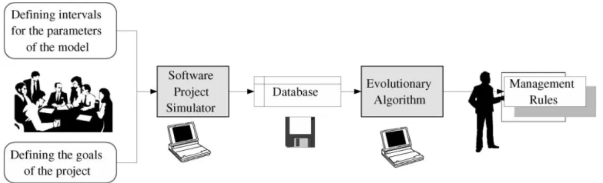
Management rules are obtained by following the steps shown in Fig. 1.
Decisions made in any organizational setting are based on what information is actually available to the decision-makers. The computer simulation tools of dynamical systems provide us with the possibility of changing one or several factors while the remaining ones are kept unchanged. The implications of managerial policies on the
0950-5849/01/$ - see front matterq2001 Elsevier Science B.V. All rights reserved. PII: S0950-5849(01)00193-8
qThe research was supported by the Spanish Research Agency CICYT
under grant TIC99-0351. * Corresponding author.
E-mail addresses: [email protected] (J.S. Aguilar-Ruiz), [email protected] (I. Ramos), [email protected] (J.C. Riquelme), [email protected] (M. Toro).
software development process could be analysed to infer the best decision.
However, a knowledge-based system might help us to determine a subset of decisions more accurately. The simulation of the project produces this knowledge with the database. Then, we only have to extract that knowledge in a comprehensible way, for example, decision lists or decision trees. In these data structures we can ®nd an easy-to-understand action to match the actual project results with the project estimations. The search for good decisions from the database generated by simulation is a highly complex task. Evolutionary algorithms provide us with a method for ®nding good solutions (in our case, decision rules) in a complex search space (database generated by an SPS) where parameters do not have an obvious relation-ship.
Other modelling techniques have been applied for estimating effort or cost of software projects: ordinary least-squares regression, analogy-based estimation [5,13,15], genetic programming [3].
2. Decision trees: C4.5
Decision trees are a particularly useful technique in the context of supervised learning. A decision tree is a classi®er with the structure of a tree, where each node is a leaf indi-cating a class, or an internal decision node that speci®es some test to be carried out on a single attribute value, and one branch and subtree for each possible outcome of the test. The main advantage of decision trees is their immediate conversion to rules easily meaningful by humans. However, classi®cation trees with univariate threshold decision boundaries might not be suitable for problems where the correct decision boundaries are non-linear multivariate functions.
The most commonly used tool is C4.5 [9], which basi-cally consists in a recursive algorithm with divide and conquer technique that optimises the tree construction on basis to gain information criterion. The program output is a graphic representation of the found tree, a confusion matrix from classi®cation results and an estimated error rate. C4.5 is very easy to set up and run; it only needs a declaration for
the types and range of attributes in a separate ®le of data and it is executed with UNIX commands with very few para-meters.
3. Evolutionary algorithm
Evolutionary algorithms (EA) are a family of computa-tional models inspired by the concept of evolution. These algorithms employ a randomised search method to ®nd solu-tions to a particular problem [6]. This search is quite differ-ent from the other learning methods. An EA is any population-based model that uses selection and recombina-tion operators to generate new sample examples in a search space. The main task in applying EAs to any problem consists in selecting an appropriate representation (coding) and an adequate evaluation function (®tness). In classical EA, the members of the population (typically maintaining a constant size) are represented as ®xed-length strings of binary digits. The length of the strings and the population sizePare completely dependent on the problem. The popu-lation simulates the natural behaviour, since the relatively `good' solutions produce offspring which replace the rela-tively `worse' ones, retaining many of the features of their parents. The estimate of the quality of a solution is based on a ®tness function, which determines how good an individual is within the population in each generation. New individuals (offspring) for the next generation are formed by using (normally) two genetic operators: crossover and mutation. Crossover combines the features of two individuals to create several (commonly two) individuals. Mutation operates by randomly changing several components of a selected indi-vidual.
Our system used an EA to search the best solutions and produced a hierarchical set of rules [11]. The hierarchy follows that an example will be classi®ed by theith rule if it does not match the conditions of the (i21)th precedent rules. The rules are sequentially obtained until the space is totally covered. The behaviour is similar to a decision list [12]. The structure of the set of rules will be as shown in Fig. 2.
As mentioned in Ref. [4], one of the primary motivations for using real-coded EAs is the precision to represent
3.1. Coding
In order to apply EAs to a learning problem, we need to select an internal representation of the space to be searched and de®ne an external function that assigns ®tness to candi-date solutions. Both components are critical for the success-ful application of the EAs to the problem of interest.
The representation of an individual takes the form shown in Fig. 3, wherelianduiare values representing an interval for the attribute. The last position (class) is the value for the class. The number of classes determines the set of values to which it belongs, i.e. if there are ®ve classes, the value will belong to the set 0, 1, 2, 3, 4.
Each rule will be obtained from this representation, but whenlimin aioruimax ai;whereaiis an attribute, the rule will not have that value. For example, in the ®rst case the rule would be [±,v] and in the second case [v,±],v being any value within the range of the attribute. If both values are equal to the boundaries, then the rule [±,±] arises for that attribute, which means that it is not relevant. Under these assumptions, some attributes might not appear in the set of rules.
3.2. Algorithm
The algorithm is a typical sequential covering EA [7]. It chooses the best individual of the evolutionary process, transforming it into a rule which is used to eliminate data from the training ®le [14]. In this way, the training ®le is reduced for the following iteration. A termination criterion could be reached when more examples to cover do not exist. The method of generating the initial population consists in randomly selecting an example from the training ®le for each individual of the population. Afterwards, an interval to which the example belongs is obtained by adding and subtracting a small random quantity from the values of the example.
3.3. Fitness function
The ®tness function must be able to discriminate between
correct and incorrect classi®cations of examples. Finding an appropriate function is not a trivial task, due to the noisy nature of most databases. The evolutionary algorithm maxi-mizes the ®tness functionffor each individual. It is given by Eq. (1)
f i 2 N2CE i1G i1coverage i 1
whereNis the number of examples being processed; CE(i) is the class error, which is produced when the example i belongs to the region de®ned by the rule but does not have the same class; G(i) is the number of examples correctly classi®ed by the rule; and the coverage of the ith rule is the proportion of the search space covered by such rule. Each rule can be quickly expanded to ®nd more examples, thanks to the coverage in the ®tness function.
4. Post-mortem analysis of a software project
The project selected for study in this paper is a personnel management system project which was carried out jointly by two local software companies. The data pertains to the design, coding and test phases. Therefore, the analysis phase and other ®nal activities are not considered. The data for initialising the parameters of the SPS were collected from the tracking documents of the original project and the experience of the project manager.
Initially, the effort expended on the project was estimated to require 208 man-days and the project was estimated to be
Fig. 3. Representation of an individual of the genetic population.
(dimensionless) MNHPXS (1±4) Most new hires per
experienced staff (tech./tech.) 1.5 MXSCDX (1±1E6) Maximum schedule
completion date extension (dim.)
5
TRNSDY (1±15) Time delay to transfer people out (days) 1 DLINCT (5±15) Average delay in incorporating
discovered tasks (days) 5 AVEMPT (500±1000) Average employment time
(days) 1000 TRPNHR (0.1±0.4) Number of trainers per new
employee (dimensionless) 0.15 UNDESM (0±50) Man-days underestimation
fraction (dimensionless) 48 UNDEST (0±50) Tasks underestimation fraction
completed in 101 days. The actual ®gures were 404 man-days and 141 days, respectively. Therefore, the underestimations of effort and time for this project were 48 and 28%, respectively. The average number of technicians involved in the project was six and the number of lines of code (LOC) was 67,800. The project manager de®ned a task as 270 LOC.
The real effort spent on the activities of development (design and coding) was 85% (404£0.85343), the rest being spent on tests. Assuming that the 10% of the effort expended on development (343£0.134) was used for revision activities, the total effort of development was 309 man-days (343234309).
Thus, the development productivity for this project was as follows:
software development productivity development effortsize in LOC 67309;800 219:4 LOC=man-days
Some interesting data from the project are shown in Table 1. Each row contains the name of the parameter in the model, the range of values it can assume, a brief description of its meaning and the estimated value at the beginning of the project. (This notation is the one used in the works of Abdel-Hamid [1].)
Several qualitative labels, which are illustrated in Table
2, were assigned to each parameter, depending on its range of numeric values. This information was provided by the project manager.
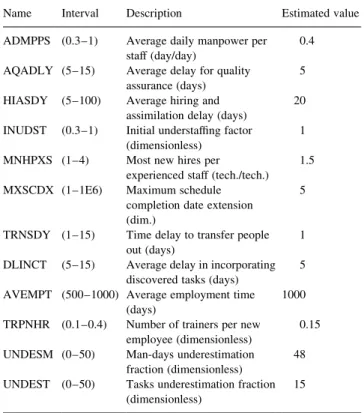
4.1. Project simulation
The evolution of the necessary effort, delivery time and pending tasks required in order to complete the personnel management system obtained by the SPS is illustrated in Fig. 4. If the results are compared with the real values, we can observe that, in the simulation the estimated delivery time is 151 days (instead of 141) and the estimated effort is 410 man-days (instead of 404). This means that the absolute percentage error was about 6.62 and 1.46%, respectively. If an SPS had been used at ®rst, we would have known the behaviour of the project, and the absolute percentage error might have been smaller. In addition, in Fig. 4 it is possible to note that the ®rst adjustments were made near the middle of the project (around 70 days) when it was detected that the number of pending tasks was greater than that expected. The decision coincided with the real evolution of the personnel management system, since more than half of the estimated time had been spent when more than half of the pending tasks remained un®nished. Time and ®nal effort might increase if the gradient of the pending tasks does not change. Two additional considerations can be observed in Fig. 4: ®rst, the estimated initial effort is modi®ed before the time, as is usual in the majority of the projects being devel-oped by the two local software-development companies; and second, the changes applied to effort and time are made simultaneously.
Data from the real evolution of the project were not collected by the companies. We only know the initial and ®nal data provided by the project manager. Therefore, if both simulated and real behaviours are compared (this was possible, thanks to the help of the project manager), we could only see that the ®nal estimated time and effort obtained by means of simulation are in agreement with the reality. This is especially true in two respects:
² The early revisions were done when half of the time had been spent.
Table 2
Qualitative description of the parameters
Name Numeric interval Qualitative description ADMPPS (0.3±0.5) Low (0.5±0.75) Average (0.75±1.0) High UNDESM (0±15) Low UNDEST (15±35) Average (35±50) High TRPNHR (0.1±0.15) Low (0.15±0.25) Average (0.25±0.40) High
² The revisions that were carried out to adjust the detected deviations affected both the time and the effort simulta-neously.
The utility of an SPS in analysing the evolution of projects carried out by our local software-development companies has been demonstrated, and generally any project could be analysed in the same way [1].
5. Management rules 5.1. The goals of the project
Two goals of the management rules that we are going to obtain are the following:
² We would wish that the values for effort were less than or equal to the value obtained by the simulation (410 man-days). These possible values are labelled as GOOD. The values greater than 410 man-days are labelled as BAD. ² We would wish that the development time were less than
or equal to the value obtained by the nominal simulation (151 days). These values are labelled as GOOD. The values greater than 151 are labelled as BAD.
5.2. Management rules from the evolutionary algorithm Management rules are obtained by the following steps (Fig. 1):
² De®ne the intervals of values for the parameters of the dynamic model (Table 1).
² De®ne the goals of the project (values for time and cost).
² Generate the database automatically. Each simulation
produces a record with the values of the parameters and
the values of the variables (cost and time) and this record is saved in a ®le.
² From the ®le generated in the preceding step, a set of management rules is provided automatically for the deci-sion-making task.
It is important to note that the ®rst two steps aforemen-tioned are performed by the project manager and the next two items are executed automatically. The management rules obtained by evolutionary algorithms for estimating simultaneously GOOD results for both time and effort are shown in Fig. 5. The number of the rule and the number of records from the database covered by the rule are shown respectively, in brackets.
The rules chosen to analyse the project are rules 1 and 2, since rule 1 covers more than half the cases forecast as GOOD and rule 2 has the smaller number of para-meters. Another good criterion for selecting the most adequate decision rule is choosing the rule having parameters which are easier to modify and control and, if possible, the rule involving the smallest number of parameters. Once the rule set is obtained, we have to select which parameters do not match the initial values. Observing Table 1, we could rewrite the management-rule set by eliminating the conditions that are matched with the initial values. The new management-rule set is illustrated in Fig. 6.
For example, in the rule 1 from Fig. 5 the values of the parameters TRP-NHR, UNDESM, UNDEST and HIASDY were initially estimated as belonging to the interval de®ned by the rule (Table 1), so that the parameters ADMPPS and INUDST must be the only ones to be modi®ed in order to obtain good results (Fig. 6), since the project is already ®nished.
Analysing the rules, we could state the following: ² Rule 1: if the average daily manpower per staff
(ADMPPS) was greater than 52% and the initial under-staf®ng factor (INUDST) was less than 96%, then the project tended to be towards GOOD.
² Rule 2: if the man-days underestimation fraction (UNDESM) was less than 37%, then the project tended to be towards GOOD (if the error in the initial necessary effort had been less than that estimated; in this project the value of UNDESM was 48%).
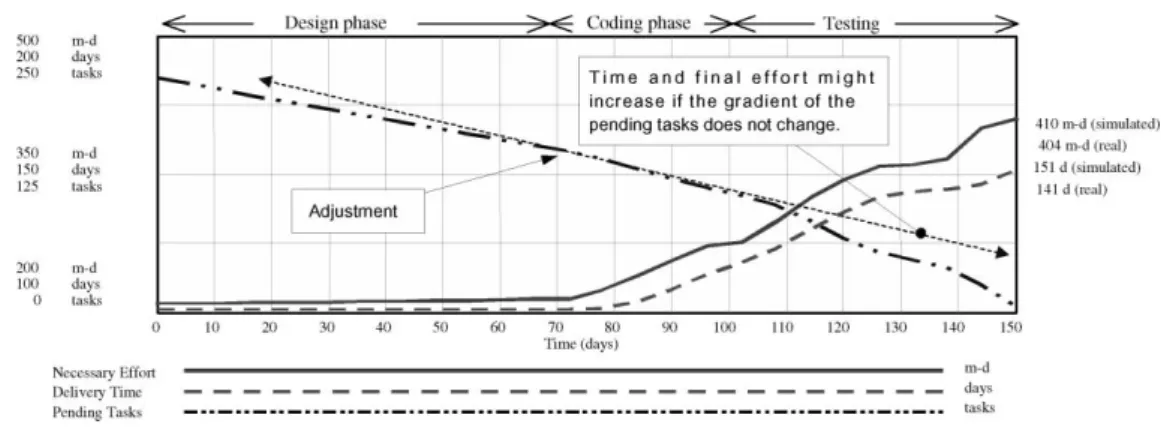
Although each rule permits good estimates, the SPS allows us to compare the results of the simulation with those which would be obtained by applying each manage-ment rule.
For example, the results obtained by the application of rule 2 are shown in Fig. 7. Both effort and time are remark-ably lower than those obtained from the simulation. In concrete terms, the necessary effort and time would be reduced to 26 man-days and 13 days, respectively, if rule 2 had been applied. With this information, the project manager decides which rule is more appropriate for achiev-ing the aims.
The SPS plays an important role in the decision-making task: ®rst, post-mortem projects can be analysed in order to infer which actions could improve the results; second, an a priori analysis would indicate the intervals within which the values of the parameters have a tendency to achieve the aims of the project.
Taking an effective decision is a very complex task. Some criteria are contradictory. For example, in general, keeping to the project deadline has highest priority, i.e. if the project schedule is at risk, more manpower will be added to the project [8]. However, the Brooks' law states that adding more people to a late software project makes it further delayed [2].
5.3. Management rules from C4.5
The management rules obtained by the C4.5 tool to esti-mate simultaneously GOOD results for both effort and time are shown in Fig. 8.
Those rules involving less number of parameter are easier to study. Analysing rule 1, GOOD results could be obtained if the number of trainers per new employee is less than 11%, the man-days underestimation fraction is less than 31 and the average hiring and assimilation delay is less than 69 days. Now we select the parameters that do not match the initial values. As we did with the rules generated by the evolutionary algorithm, we could rewrite the management-rule set by eliminating the conditions that are matched with the initial values from Table 1. The new management-rule set is shown in Fig. 9.
5.4. Comparing the results obtained by the evolutionary algorithm and C4.5
In general, the evolutionary algorithm is more accurate in ®nding solutions in the search space. This can be observed examining the number of examples from the database that have been covered and the percentage over the total number of GOOD examples (Table 3).
Fig. 7. Results obtained by applying rule 2.
The best rule obtained by C4.5 contains 6 (GOOD) exam-ples. However, the best of the evolutionary algorithm contains 21 (GOOD) examples. For our analysis, the more accurate rule is that which is capable of covering greater number of GOOD examples. Therefore, rule 1 from the evolutionary algorithm is much better than any rule obtained by C4.5. In addition, the total number of GOOD examples covered by the evolutionary algorithm is about 90% with four rules, in comparison to the ®ve rules required by C4.5 to cover about 63%.
6. Another approach
In Section 5, we saw how an evolutionary algorithm auto-matically provides management rules from a database generated by an SPS. Another interesting approach consists in presenting graphically the relationship between two para-meters in the cases in which good results were obtained. These graphics inform the project manager about the range of values for the parameters being analysed. An exam-ple of this kind of analysis is shown in Fig. 10, where the parameters TRPNHR and ADMPPS are compared, indicat-ing when the effort and the time are simultaneously good. In Fig. 10, each axis is a parameter of the model and each case labelled as GOOD (in the database) is represented by a point
7. Conclusions
The use of simulators and systems that learn decision rules helps to estimate software projects and to produce management rules automatically for the decision-making task. These management rules could be applied:
² Before the project has begun: de®ning more adequate managerial policies.
² After the project has ®nished: doing a post-mortem analysis.
² When the project is running: taking immediate decisions (monitoring).
Management rules make it possible to:
² obtain values considered as good (very good, normal, bad, etc.) for any variable of interest (time, effort, quality, number of technicians, etc.), independently or together with other variables;
² analyse managerial policies capable of achieving the aims of the project;
² know to which range of values the parameters must belong in order to obtain good results.
In short, it is possible to generate management rules auto-matically for any software project and to know the manage-rial policies that ensure the achievement of the initial aims. The deviations from the initial forecast could be detected (monitoring) and the behaviour of the process is well under-stood through the management-rule set.
Evolutionary computation provides an interesting approach for dealing with the problem of extracting knowledge from
Comparing the number of examples covered by the rules
Rule 1 2 3 4 5 Total
C4.5 5(12%) 6(14%) 5(12%) 5(12%) 5(12%) 26(63%) EA 21(51%) 7(17%) 6(14%) 3(7%) ± 37(90%)
databases generated by SPS. The quality of the set of rules produced by the evolutionary algorithm has been compared to those generated by C4.5. The results demonstrate that our approach ®nd better solutions in the search space, covering more GOOD examples with less number of rules. And, what is more important, is that the results (management rules) are applicable and bene®cial.
The authors consider that this technique contributes to coping with the complex problem of decision-making within the software project development framework, and it facilitates the use of dynamic models, since the project manager only has to provide the aims of the project and the range of the parameters, especially for those having a high degree of uncertainty. We are currently working on the application of other machine learning techniques (fuzzy logic, association rules, etc.) to the databases generated by the SPS.
Acknowledgements
The authors are grateful to J.J. Dolado for helpful comments and to the reviewers for their suggestions. References
[1] T.K. Abdel-Hamid, Software Project Dynamics: An Integrated Approach, Prentice-Hall, Englewood Cliffs, NJ, 1991.
[2] F.P. Brooks, The Mythical Man Month, Addison-Wesley, Reading, MA, 1978.
[3] J.J. Dolado, On the problem of the software cost function, Information and Software Technology 43 (2001) 61±72.
[4] L.J. Eshelman, J.D. Schaffer, Real-coded genetic algorithms and interval-schemata, Foundations of Genetic Algorithms 2 (1993) 187±202.
[5] G.R. Finnie, G.E. Wittig, J.-M. Desharnais, A comparison of software effort estimation techniques: using function points with neural networks, case-based reasoning and regression models, Journal of Systems and Software 39 (3) (2000) 281±289.
[6] D.E. Goldberg, Genetic Algorithms in Search, Optimization and Machine Learning, Addison-Wesley, Reading, MA, 1989.
[7] T. Mitchell, Machine Learning, McGraw Hill, New York, 1997. [8] D. Pfahl, K. Lebsanft, Using simulation to analyse the impact of
software requirement volatility on project performance, Information and Software Technology 42 (2000) 1001±1008.
[9] J.R. Quinlan, C4.5: Programs for Machine Learning, Morgan Kauf-mann, San Mateo, California, 1993.
[10] I. Ramos, J.S. Aguilar-Ruiz, J.C. Riquelme, M. Toro, A new method for obtaining software project management rules, Proceedings of VIII Software Quality Management (2000) 153±164.
[11] J.C. Riquelme, J.S. Aguilar-Ruiz, M. Toro, Discovering hierarchical decision rules with evolutive algorithms in supervised learning, Inter-national Journal of Computers, Systems and Signals 1 (1) (2000) 73± 84.
[12] R.L. Rivest, Learning decision lists, Machine Learning 1 (2) (1987) 229±246.
[13] M. Shepperd, C. Scho®eld, Estimating software project effort using analogies, IEEE Transactions on Software Engineering 23 (12) (2000) 736±743.
[14] G. Venturini, Sia: a supervised inductive algorithm with genetic search for learning attributes based concepts, Proceedings of European Conference on Machine Learning (1993) 281±296. [15] F. Walkerden, R. Jeffery, An empirical study of analogy-based
soft-ware effort estimation, Empirical Softsoft-ware Engineering 42 (1999) 135±158.