Wind Power Potential Analysis Based on Different Methods Fitted in Weibull and Rayleigh Models for Wind Patterns in Juja and Naivasha

Wind Power Potential Analysis Based on

Different Methods Fitted in Weibull and

Rayleigh Models for Wind Patterns in Juja

and Naivasha

Maina Anne Wandia

1

, Kamau Joseph Ngugi

1

, Timonah Nelson

1

, Nishizawa Y

2

, Churchill Saoke

1

Researcher, Department of Physics, Jomo Kenyatta University of Agriculture and Technology 1 Researcher, Ashikaga Institute of Technology, Japan 2

ABSTRACT: The wind speed characteristics of Juja, (altitude of 1416 m above sea level; 10 10’ S, 370 7’ E), Kenya was analysed at heights of 10 m and 30 m. The wind speed averages at 10 m and 30 m were found to be 2.54 m/s and 3.04 m/s, respectively. The wind shear exponents and roughness parameters were analysed and found to be 0.1652 and 0.0374 respectively. Weibull scale and shape parameters were obtained using Weibull-fit, Regression and the Maximum Likelihood. Wind speed modelling was done using the Weibull and Rayleigh probability distribution functions. Power densities for different methods were calculated. Results obtained from Juja site were compared with results acquired from Naivasha, St. Xavier site which is at an altitude of 2,086 m; 0° 43' 0" S, 36° 26' 0" E. The mean wind power densities for Juja (10 m and 30 m) and Naivasha (10 m) were 12.68 W/m², 20.65 W/m² and 39.95 W/m² by Weibull model and 14.51 W/m², 22.43 W/m² and 28.63 W/m² by Rayleigh model respectively. The Weibull-fit and Maximum Likelihood fitted best Juja site and Naivasha site respectively

.

KEYWORDS: Wind power density, Wind distribution models, Wind direction, Wind speed

I. INTRODUCTION

Juja, 1416 m above sea level (10 10' S, 370 7' E) and about 35 km from Nairobi, is a region that has a rapidly growing population and a major University, Jomo Kenyatta University of Agriculture and Technology (JKUAT). On the other hand, Naivasha, 2,086 m (0° 43' 0" S, 36° 26' 0" E), is an area congested with agricultural farms. These two areas require an alternative energy source to supplement existing convectional energy. Use of power generators during power outage leads to air pollution and hence the need for clean, reliable, sustainable and cost effective sources. Wind energy is among the least exploited with 25.5 MW from the two Ngong wind farm phases, though there are underway processes of establishing other wind plants in Kenya such as in Turkana [4].

Thorough wind speed analysis in this area is therefore critical. A research based on different methods brings out a better picture of the state of wind in a site. The power available in wind is basically dictated by the wind speed. To obtain power from the wind, the force of the wind is harvested by the rotors of a wind turbine. Basically, the force on the wind is converted to a torque [5]. The power of the wind is proportional to the cube of wind velocity, the rotor area and the air density. This relation is shown in equation 1. It is however worth noting that the nature of the terrestrial surface including artificial obstacles such as hills, trees and buildings affects the wind speed.

Several methods and Probability Density Functions (PDFs) have been used in literature to describe wind speed characteristics. The methods include Weibull-fit, Regression, Standard deviation, Maximum Likelihood, Chi-square among others while PDFs include Weibull, Rayleigh, bimodal Weibull, lognormal and gamma among others [2]. The tabulations and mathematical formulas of these relationships are well described and explained in the procedures of analysing the bulk wind speed data. This paper analyses wind speed using different methods modelled using Weibull and Rayleigh models for Juja and correlates them with results from Naivasha, St. Xavier site within a period of three months.

III. MATERIALS AND METHODS

The study was carried out in Juja at 10 m and 30 m heights in order to measure wind speeds and directions at the two heights above the ground. A mask of required length was constructed using metallic circular tubes. Anemometers (Ultrasonic wind sensors) were clamped on the mask at 10 m and 30 m in order to measure wind speeds and directions at these heights above the ground. The sensors were connected to transmitting devices (clamped on metallic rods) using insulated cords. The transmitters were linked with two Ultrasonic data loggers programmed so as one received data from 10 m and the other from 30 m centres. The data (diurnal averaged wind speed/direction and temperature) was stored in computer memory (disc) awaiting processing. The averages of wind parameters were obtained daily for three months. The wind shear exponents,



surface roughness

z

₀, Weibull scale parameter c, shape parameter k and power densities were determined. Wind power potential was modelled using Weibull and Rayleigh distributions functions. The results were compared to acquired results from Naivasha, for the same months.

Theory

The analysis of wind parameters was done using the following procedures;

Power available in the wind

Where; ...1 p a RT  ;

P

is air pressure,

R

gas constant and,

T

temperature in degrees Kelvin.

The wind velocity at the rotor plane is the average of upstream and downstream wind speeds. Maximum useful power is given by Betz’s constant 0.59.

The power law

Wind speed near the ground changes with height; this involves an equation that forecasts wind speed at different height by using the available wind speed data. The most commonly used equation for the variation of wind speed with height is the power law [6] is;

1 2 2 1

...2

h

v

v

h







  





Where

v

₁ (m/s) is the actual wind speed recorded at height

h

₁ (m), and

v

₂ (m/s) is the wind speed at

h

₂(m). The exponent



depends on the surface roughness and atmospheric stability. Wind shear exponent, a difference in wind speed and direction vertically has been determined for various types of terrains [7].

Roughness length,

z

₀ which is used to characterize shear and the height above the ground is not constant [8] and thus equation 2 can be modified to yield equation 3.

 

 

2 0 1 0 h z 2 1 h

z

ln

...3

ln

v



v

Wind probability distributions

Two of the commonly used functions for fitting a field data probability distribution in a given location over a certain

period of time are the Weibull and Rayleigh distribution models [9]. The Weibull probability density function

,

f

_R

 

v

is given as;

 

exp

...

...

...

4

1 k k R

c

v

c

v

c

k

v

f































 

₃

exp



...

...

...

5











c

c

v

f

R

Methods of Obtaining Weibull Parameters

Maximum Likelihood (MLH)

The parameters k and c (m/s) can be estimated by using the Maximum Likelihood Method [10, 11] as;

 

 

1

1 1 1

ln

ln

...6

n n k

i i i

i i

n k i i

v

v

v

k

n

v

   



































1 2 1

1

...7

2

n k i i

c

v







 









Weibull-fit

The shape and scale parameters as per Weibull-fit are as follows [11].

...8

1

1

m

v

c

k







 

_

_





1.090

...9

v m

k

v









 







Where



_yis standard deviation and

v

_m, the mean wind speed.





1 2 2 1 1

...11

n

i i m i

y n

i i

f v

v

f



 



_





























Regression

The cumulative probability function of the Weibull distribution [12] is given by;

 

1 exp ...12

k v F v c  _{ }    _{ }       

To determine k and c requires a good fit of the equation above to the recorded discrete cumulative frequency function. By taking the natural logarithm of both sides of equation 12 twice gives;

ln



ln[1



F v

( )]



k

ln( )

v



k

ln ...13

c

Plotting

ln



ln[1



F v

( )]

against ln( )v Presents straight line whose gradient is k and the y-intercept is klnc from which

c

can be calculated.

Wind Power Density Function

The evaluation of wind power per unit area

P

_v is of fundamental importance in assessing wind power projects [13, 16].

The formula for

P

_v is given by;

 

3 1

1

...14

2

n v i i

P

v

n









Where the wind speed at stage i, is

v

_i, n, the number of non-zero wind data points and ρ, is air density. The ρ depends on altitude, air pressure and temperature and is approximated to be 1.225 kg/m3 at Juja. The expected monthly or annual wind power density per unit area of a site based on Weibull Probability Density Function

P

_W [12] can be

expressed as follows;

3

1

3

1

...15

2

W

P

c

k









 

_

_





The two significant parameters k and c are closely related to the mean value of the wind speed

v

_m[14]. By extracting c

from equation 15 and setting k = 2, the power density for the Rayleigh model

 

P

_R is found to be;

 

3

3

...16

R

v

m

P

_

Where:

3

0.88623 ...17 2

m

V  c  _{ } c

 

IV. RESULTS AND DISCUSSION

Wind Shear

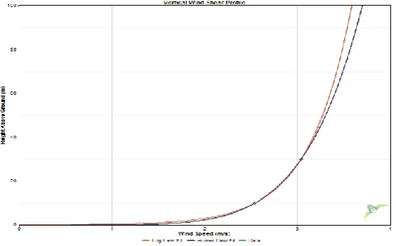
Average diurnal wind speeds, wind directions, and temperatures were obtained for three months. The average wind speeds for Juja at 10 m and 30 m heights were 2.54 m/s and 3.04 m/s respectively. Wind shear exponent and roughness parameters for Juja were 0.1652 and 0.0374 respectively. These parameters are in line with Linacre and Geerarts 1999, [7]. The wind shear profile was obtained by use of Windographer software (figure 1). Diurnal variation for the whole period of three months is shown by figure 2.

Figure 1: Wind shear profile

Diurnal variation of average wind speeds and directions

Diurnal variation of average wind speeds was obtained by use of Microsoft Excel and was as per figure 2.

Figure 2: Diurnal variation of wind speeds, March - May, 2015

The two sites had low wind speeds of wind class 1, though wind speeds in March and at the beginning of May, were slightly higher as observed in figure 2. This can be attributed to higher temperatures which led to increase in pressure gradient. The diurnal profile portrays higher wind speeds in Naivasha than Juja site for the three months. Since the wind flow patterns are modified by the earth’s terrain, bodies of water and vegetative cover which determine the degree of roughness, [5, 13] higher wind speeds in Naivasha can be attributed to the effect of the lake Naivasha and channelling effect of the Rift valley and the hills.

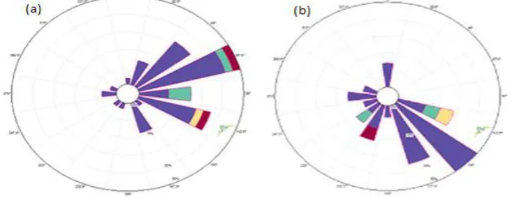
WindRose Diagrams

WindRose diagrams were used to analyse wind direction as shown by figure 3. Most Juja wind was between east north east (ENE) and east south east (ESE) while that of Naivasha was between south east (SE) and south west (SW).

Weibull Parameters, Probability Density Functions and Power Densities

The wind speeds were used to determine Weibull shape parameters (k), scale parameters (c), (table 1), and wind power densities, (table 2) for different methods. Windographer software and Microsoft Excel were used to determine and generate the parameters and Probability Distribution Functions (PDFs).

Table 1: Weibull parameters for different methods

Method At a height of 10 m(Juja site) At a height of 30 m (Juja site) Naivasha (St. Xavier)

c (m/s) k c (m/s) k c (m/s) k

Weibull-fit 2.811 2.937 3.646 _3.394 4.209 2.390

Regression 2.937 2.773 2.937 2.773 2.718 1.810

MLH 2.394 1.261 2.652 0.943 2.635 0.943

Actual power densities for 10 m and 30 m in Juja and 10 m, in Naivasha were 14.5 W/m², 30.9 W/m² and 58.5 W/m² respectively. The mean wind power densities for Juja (10 m and 30 m) and Naivasha (10 m) were 12.68 W/m², 20.65 W/m²and 39.95 W/m² by Weibull model and 14.51 W/m², 22.43 W/m² and 28.63 W/m² by Rayleigh model respectively. Error analysis was done using equation 18.

( , ) ( , ) ( , )

(%) W R M R ...18

M R

P P

Error

P

 

Where

P

_{W R, } in (W/m2) is the mean power density calculated from either the Weibull or Rayleigh function used in the

calculation of the error and _{ }

,

M R

P

is the wind power density for probability density distribution derived from field data

values which serve as the reference mean power density.

Table 2: Wind power densities

Month Wind Power Density (W/m²)

At 10 m(Juja site) At 30 m(Juja Site) At 10 m(Naivasha site)

W EW R ER W EW R ER W EW R ER

Weibull-fit 13.81 -0.05 16.88 0.16 22.44 -0.27 36.85 0.19 36.54 -0.38 56.70 0.03 Regression 13.73 -0.06 16.21 0.08 18.81 -0.39 19.26 -0.38 18.42 -0.69 15.27 -0.74 MLH 10.50 -0.28 10.43 -0.28 20.70 -0.33 14.18 -0.54 64.90 0.10 13.91 -0.76

Probability Distribution Functions (PDFs)

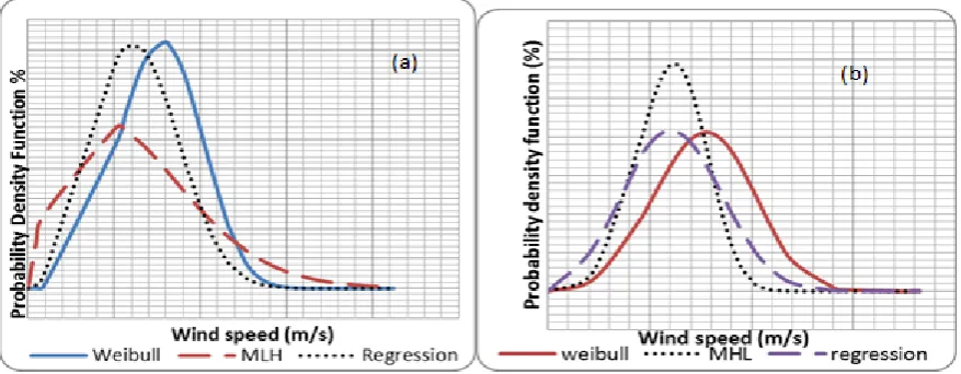
The Probability Distribution Functions generated from Weibull parameters obtained from different methods are as per figures 4 and 5 (a) and (b). The area under each PDF curve represents power density.

Figure 4: Probability Distribution Functions (PDF) s, 10 m, Juja

The curves portray that different methods of analysis yielded different values of power densities for the same site. This can be attributed to conditions under which each method was established.

Figure 5: Probability Distribution Functions (PDF) s, (a) 10 m, Naivasha (b) 30 m, Juja

The results on power density showed Weibull-fit being the method of best fit for Juja and Maximum Likelihood for Naivasha by Weibull distribution model while Regression fits Juja best and Weibull-fit, Naivasha, by Rayleigh model. This implies that power density, for any selected site, should be obtained using different methods in order determine the actual state of wind in the site.

V. CONCLUSION

The results indicated that different methods of analysis yield different values of power density and that method of best fit is dependent on locality/ altitude as per Paitoon, 2010s’ [15] findings. From the windRose analysis, most winds for Juja site were found to be in the North East and East South East directions while those for Naivasha were between South East and south west directions. The two sites were found capable of power generation by use of small horizontal axis wind turbines such as ModernVestas turbines with cut-in speed of 2.5 m/s. The generated power can be used for activities such as battery charging and water pumping.

ACKNOWLEDGEMENTS

I acknowledge BRIGHT PROJECT, Phy.Dept (JKUAT), Prof. Nyende, Saoke C., Samuel M. and Ngei Katumo.

REFERENCES

[1]. Kamau, J.N., Kinyua R., and Gathua, J.K.: “6 years of wind data for Marsabit, Kenya average over 14m/s at 100m hub height; an analysis of the wind energy potential”. Renewable Energy, Vol. 35,No. 6 Pp. 1298-1302, 2010

[2]. Kollu, R., Rao, S., Rayapudi, M., Narasimham, S. And Pakkurthi, K.M., “Mixture probability distribution functions to model wind speed distributions”. International Journal of Energy and Environmental Engineering, Vol. 27, Pp. 2251-6832, 2012.

[3]. Ajayi, O.O., Fabenle, R.O., and Katende, J. (2011).Wind profile characteristics and econometrics analysis of wind power generation of a site in Sokoto state, Nigeria. Energy Science and Technology, Vol. 1, Pp. 54-66, 2011.

[4]. Mbogo, S., “Works- on- 300MW Turkana Wind Farm Start". The East African, (Nairobi). 2015. Retrieved 25 April 2015

[5]. Saoke, C.O.: “Analysis of wind speeds on Weibull and data correlation for wind pattern description for a selected site in Juja”.M.Sc. thesis, Jomo Kenyatta University of Agriculture and Technology, Juja, Kenya, 2011.

[6]. Kantar, Y.M., and Usta I., :“Analysis of wind speed distributions function derived from minimum cross entropy principles as better alternative to Weibull function”. Energy conversion management. Vol. 49, Pp. 962-973, 2008.

[7]. Linacre, E. and Geerarts, B.: “Roughness length”. 1999. Available at: http//www-das.uwyo.edu/~geerts/cwx/notes/chap14/roughness. Retrieved 8 October 2015

[8]. Manwell, J.F., McGowan J.G., and Rogers A.L.: “Wind energy explained Theory, design and application". John Wiley and sons Ltd. West Sussex, United Kingdom, 1999.

[9]. Kantar, Y.N., and Senoglu B.: A comparative study for the location and scale parameters of the Weibull distribution with given shape parameter. Computer Geoscience, Vol. 34, Pp. 1900-1909, 2008.

[10]. Zhang, L.F.., Xie, M., and Tang, l. C.:“Robust regression using probability plots for estimating the Weibull shape parameter”. Quality reliability Engineering International. Vol. 22, Pp. 905-917, 2006.

[11]. Justus, C.G., Hargraves, W.R., Mikhail, A. and Graber, D.: “Methods of estimating wind speed frequency distributions”. Journal of Applied Meteorology,Vol. 17, Pp. 17-18, 1978

[12]. Akpinar, E. K., and Akpinar, S.:“Statistical analysis of wind energy potential on the basis of Weibull and Rayleigh distribution for Agin-Elazig, Turkey. Proceedings of the Institution of Mechanical Engineer’s”. Journal on Power and Energy. Vol. 213, Pp. 557-563, 2004. [13]. Wieringa, J. Representative Roughness parameters for homogeneous terrain. Boundary Layer Meteorology. Vol.63, Pp. 323-362, 1993.

[14]. Lun, Y. F., Lam, C. A Study of Weibull Parameters using long term wind observations. Renewable Energy, Vol. 20 Pp. 145-153, 2000. [15]. Paitoon, S.:“Demonstrating-Measure-Correlate-predict algorithms for Estimation of Wind Resources in Central Finland”. MSc. thesis,

University of Jyvaskyla, Finland, 2010.

[16]. Zhou, J., Erdem, E., Li, G. and Shi, J.: “Comprehensive evaluation of wind speed distribution models: A case study for North Dakota sites”.