Modelling credit card customer behaviour

i

Modelling Credit Card Customer Behaviour

Sara Barradas Pereira

Work Project presented as a partial requirement for the

Degree of Master of Statistics and Information Management,

with a specialization in Information Analysis and Management

March 2019

i

Management School

Instituto Superior de Estatística e Gestão de Informação

MODELLING CREDIT CARD CUSTOMER BEHAVIOUR

by

Sara Barradas Pereira

Work Project presented as a partial requirement for Degree of Master of Statistics and Information Management, with a specialization in Information Analysis and Management

Supervisor: Ana Cristina Costa

ii

DEDICATION

O presente trabalho é totalmente dedicado às pessoas que me têm dado apoio incondicional ao longo da minha vida e que em seguida mencionarei. Em primeiro lugar queria agradecer às três pessoas mais importantes da minha vida que são a minha mãe Isabel Pereira, o meu pai Carlos Pereira e o meu irmão Ricardo Pereira, sem o apoio deles seria impossível ter traçado o caminho da forma que tracei! Sem dúvida que tenho a maior sorte do mundo em tê-los comigo e quero agradecer muito a paciência, persistência e dedicação deles em tentarem sempre trazer o melhor de mim ao de cima e tentarem sempre ajudar-me em tudo o que conseguem. Gostava também de mencionar os meus avós maternos (Maria Clarisse e José Barradas) e paternos (Hermínia e Antero Bento) pelo orgulho gigante que tenho por eles e por sentir, sem sombra de dúvida, o mesmo da parte deles! Não podia deixar de mencionar a minha tia Luísa Barradas e a minha amiga Inês Fonseca, que foram um contributo essencial para o meu crescimento pessoal e emocional ao longo destes dois últimos anos. Quero também agradecer a todos os meus amigos que de uma maneira ou de outra estiveram sempre presentes nas fases que eu mais precisei, e eles sabem quem são.

iii

ACKNOWLEDGEMENTS

A realização deste trabalho de projeto não teria sido possível sem o contributo de algumas pessoas. Agradeço muito toda a colaboração prestada pela minha orientadora, Professora Ana Cristina Costa, através das sugestões dadas e dos vários esclarecimentos a todas as questões que fui colocando ao longo da construção deste trabalho. Um agradecimento especial à minha chefe, Maria Goulão, que, em conjunto com as necessidades da empresa, permitiu o desenvolvimento deste projeto. Gostaria também de agradecer ao Professor Jorge Mendes que através das aulas da cadeira de Metodologias de Investigação me mostrou caminhos para tornar este trabalho mais rico. Foi, também, através de uma prática utilizada nesta cadeira que obtive um feedback muito interessante de um colega em particular, o Tiago Lopes, através dos seus pertinentes comentários sobre as diversas fases do meu trabalho, e que muito contribuíram para a sua melhoria. Por fim, mas não menos importante, queria agradecer à minha colega Telma Correia que, com o seu conhecimento mais avançado sobre determinados assuntos relacionados com o tema do presente trabalho, me foi dando algumas sugestões importantes.

iv

ABSTRACT

Credit cards have great influence over consumers’ daily lives, mainly because they provide functionalities that other financial products do not. Studies have been performed in order to research over which are the best clients. To put it in other words, which clients spend more money with credit cards. The aim of this study is to understand the behavior of a credit card consumer depending on whether they do or not many payment transactions with a huge amount of money. With this objective a logistic regression model was investigated, based on many potential explanatory variables (socio-demographic variables, customer profile in the company and customer profile in Banco de Portugal). Several diagnosis tests and goodness of fit tools were used to select the final model, which allows to forecast the client type behavior based on 10 variables. Results show that clients who live in Central North and Central region of Portugal, who have Plafond between 1500 and 9000 euros, who are homemaker or student, who receive cashback and who have seniority in the company between 32 and 84 days ago are the best clients for our case study. We expect that with the proposed model, the company1 _{will know how to appropriately manage each specific client and its needs.}

KEYWORDS

Customer behaviour; credit card; payment transactions; descriptive statistics; logistic regression.

v

RESUMO

Os cartões de crédito têm uma grande influência no dia-a-dia dos consumidores, principalmente porque fornecem benefícios que outros produtos financeiros não oferecem. Alguns estudos foram realizados com o objetivo de pesquisar quais são os melhores clientes. Por outras palavras, quais são os clientes que gastam mais dinheiro com a utilização do cartão de crédito. O objetivo deste estudo é entender o comportamento de um consumidor de cartão de crédito, dependendo se ele faz ou não muitos pagamentos de transações e se os mesmos são de elevado valor. Com este objetivo, foi proposto um modelo de Regressão Logística com base em potenciais variáveis explicativas (como por exemplo variáveis sociodemográficas, perfil do cliente na empresa2 _{e perfil do cliente no Banco de}

Portugal). Diversos testes de diagnóstico e ferramentas de “goodness of fit” foram utilizados para selecionar o modelo final, o que permitiu prever o comportamento do tipo de cliente com base em 10 variáveis. Os resultados mostram que os clientes que vivem na região Centro Norte e Centro de Portugal, que têm Plafond entre 1500 e 9000 euros, que são donas de casa ou estudantes, que recebem cashback e que têm uma antiguidade na empresa entre 32 e 84 dias são os melhores clientes para o nosso caso estudo. Esperamos que, com o modelo proposto, a empresa saiba como acompanhar adequadamente cada cliente e as suas necessidades.

PALAVRAS-CHAVE

Comportamento do cliente; cartão de crédito; pagamentos de transações; estatística descritiva; regressão logística.

vi

INDEX

Abstract……….…iv

1

Introduction ... 1

1.1

Background ... 1

1.2

Problem Identification and Study Relevance ... 2

1.3

Study Objectives ... 3

2

Literature Review ... 4

2.1 Credit Cards Usage ... 4

2.2 Credit Card Default and Fraud ... 6

3

Methodology ... 8

3.1

Definition of the study variable ... 8

3.2

Data Set ... 8

3.3

Definition and construction of explanatory variables ... 9

3.4

Discriminant Univariate Analysis ... 9

3.5

Multicollinearity Analysis ... 9

3.6

Logistic Regression ... 10

3.6.1 Univariate Logistic Regression ... 10

3.6.2

Multiple Logistic Regression ... 13

3.6.3

Variables Selection ... 14

3.6.4

Model Diagnosis ... 14

4.

Results and Discussion ... 18

4.1 Descriptive Analysis ... 18

4.2

Discriminant Univariate Analysis ... 19

4.3

Logistic Regression - Multivariate Analysis ... 21

4.4

Multicollinearity Analysis ... 23

4.5

Model Diagnosis ... 25

4.5.1 Hosmer-Lemeshow Test ... 25

4.5.2 Deviance and Pearson Tests ... 25

4.5.3 ROC Curve ... 25

4.6

Coefficients Interpretation ... 27

5

Conclusions ... 30

References ... 32

vii

INDEX OF FIGURES

Figure 1 - Distribution of sample individuals by gender ... 18

Figure 2 - Distribution of sample individuals by marital status ... 18

Figure 3 - Distribution of sample individuals by age ... 19

Figure 4 - Distribution of sample individuals by payment method... 19

Figure 5 - ROC Curve for the Regression Model ... 26

Figure 6 - ROC Curve for the validation sample Regression Model ... 27

viii

INDEX OF TABLES

Table 1 - Contigence Table ... 16

Table 2 - Definition of dummy variables ... 21

Table 3 - Stepwise Selection variables ... 21

Table 4 - Definition of dummy variables chosen by the Regression Model ... 22

Table 5 - Results of Likelihood ratio test, Score test and Wald test ... 22

Table 6 - Analysis of Maximum Liklihood Estimates ... 23

Table 7 - P-values of the Pearson Chi-Square test applied to the variables of the Regression

Model ... 23

Table 8 - Collinearity Statistics ... 24

Table 9 - Collinearity Diagnosis ... 24

Table 10 - Partition for the Hosmer and Lemeshow Test ... 25

Table 11 - Hosmer and Lemeshow Goodness-of-Fit ... 25

Table 12 - Deviance and Pearson Goodness-of-Fit Statistics ... 25

Table 13 - Contingence table ... 26

Table 14 - Ratios about sensitivity and specificity ... 26

Table 15 - Contingence table for validation sample ... 27

Table 16 - Ratios about sensitivity and specificity for validation sample ... 27

ix

LIST OF ACRONYMS AND ABBREVIATIONS

ATM Automated Teller Machine

BdP Banco de Portugal

HMM Hidden Markov Model

MAE Mean Absolute Error OR Odd Ratio

POS Point of Sales or Point of Service RMSE Root Mean Squared Error

ROC Receiver Operating Characteristic SAS Statistical Analysis System

1

1

INTRODUCTION

1.1

B

Payment cards were introduced in 1930 in the United States of America to allow for payments at a merchant's own outlet, primarily in the "travel and entertainment" sector. Later, in the 1950s, Diners Club created the first credit card with a more general purpose (European Central Bank, 2014). This credit card company would charge an annual fee and send the monthly or annual accounts of the expenses incurred to the respective holders. In 1958, American Express launched its first card, and in the same year, Bank of America introduced BankAmericard as a consequence of discovering that the bank was losing this market, with the cardholder's innovation being able to repay its debt until the deadline. The success was immediate and the card became the most popular among those from the United States of America. Quickly, other banks joined the BankAmericard system, which gained international breadth. In 1977, BankAmericard was renamed Visa (Stearns, 2016). In Portugal, the first bank card appears in Banco Sotto Mayor, in 1970.

A credit card is a form of electronic payment and it is typically used to purchase products or services, in installments. The cardholder can make purchases up to a maximum limit implicit in the credit card contract. When requiring a credit card, there are three things to select: the plafond, the duration and the desired type of payment for the plafond. As long as the monthly payments are successfully made, the plafond will always be available. There are several brands associated to this type of cards. However, the most used in Portugal are VISA, MasterCard and American Express. The main advantages of this payment instrument for the cardholders are (Chakravorti, 2003; Chakravorti & To, 2007):

• There is no need to have a certain amount available at the moment of purchase of the product or service;

• Extended terms for installment payments; • Exemption from annuity (in some cases);

• Exemption of interest payment for debt payments done within value amount of 50 (and in certain cases the option to pay purchases in 12 months without any interest charged may be available);

• Worldwide usage;

• Serve as confirmation for online reservations and/or for payment of some products online. Many studies have been done on credit cards such as bank studies (Koparal & Calik, 2014; Pulina, 2011), monetary studies (Geanakoplos & Dubey, 2010), macroeconomic studies (Banka, n.d.; Yüksel, 2016), industrial organizational studies (Agarwal, Driscoll, Gabaix, & Laibson, 2011; Kyalo, 2012), financial economic studies (Elliehausen & Hannon, 2018) and others. Studies over credit card consumer behavior are conducted since 2006 (Kurtulus, 2006; Pulina, 2011).

2

1.2

P

I

S

R

Nowadays credit cards are a very common tool used by Portuguese individuals and families. This financial instrument allows people to make payments through a credit line, i.e., the plafond that has been previously contracted with the banking institution. The duration of this contract is unlimited and the general rule is that it is automatically renewed. These last features are precisely what distinguishes credit cards from other financial products such as personal credit or car credit. Credit cards may have two features, credit or debit. Two payment options are available: paying the total balance used at the deadline or paying partially the balance at the deadline with a required amount, a minimum amount or percentage. After customers raise their credit card plafond, they could do the following:

1. Withdraw money from an ATM (Automated Teller Machine);

2. Make purchases at any kind of store as long as the store has a POS (Point of Sales or Point of Service) terminal;

3. Transfer money from their credit card account to their current account. This report is focused specifically on ATM and POS transactions.

In order to select a credit card, there are several variables that need to be considered, which may vary between banks and even within each bank. Therefore, it is very important to properly compare different offers proposed by the market, so that the final choice will plainly suit all needs and expectations of the potential cardholder.

The following features need to be always extensively examined, before purchasing any credit card: 1. Annuity costs;

2. Interest rates and associated services;

3. Benefits provided by the bank through its usage; 4. Insurance associated.

Hence, the choice between a credit card and other financial products will mainly depend on clients' personal and specific needs, on the reason generating a need for credit and on the amount required. If a generic customer would need a certain amount (up to 1000 €) to be available at any time and for any eventuality that may arise (e.g. buying a new computer, doing the monthly shopping, paying for the car arrangement and so on), the best option is undoubtedly a credit card, since whenever the person pays for the installments, the ceiling will automatically become available. On the other hand, if the customer needs a particular amount to provide for housing works (such as € 5000), it would be better to opt for a different financial product, for example: a personal loan. Although these characteristics are extremely relevant, the financial company3 _{that provided the data for this project}

has only limited information about the customers who purchased the credit card. This study originates from the need of the company to have its first analysis made about their clients given that the credit card is a very recent and new product in their service portfolio. The main goal is to analyse the

3 behaviour of clients that make several financial transactions with their credit card after an account is opened.

Within the company there are only profile studies about other financial products such as personal credit or car credit. These studies were mainly based on scores that provide a mere glimpse of what is a typical "good" client for each product. Since a credit card is a financial product, any study about “old financial products” that this company has, could be very similar in its conceiving. However, given that credit cards can present diverse features, the studies have to highlight these dissimilarities. For this reason, modelling the behavior of credit card consumers depending on whether they do, or not, many payment transactions with large amounts of money is of crucial importance. With the resulting information, the company could be able to improve the offers and enhance the contract options for its clients.

1.3

S

O

This study was being developed in the Marketing Department of the financial company with the objective to prepare more accurate and effective “actions” for clients categorized as "the best" and provide them an appropriate marketing experience. This research aims to evaluate which variables better define the client who makes “many” financial transactions with a significant value with their credit card. In other words, the main objective is to investigate a model characterizing “Good” and “Bad” clients, based on their financial transactions and sociodemographic characteristics. Since the credit card is a new product of this company and thus the quantity of data is modest, for the moment it is just possible to evaluate clients based on limited information, e.g. financing or not financing. The variables that will be studied are based on internal information such as sociodemographic characteristics, company behaviour about other financing products and external information, provided by Banco de Portugal (central bank of Portugal). To achieve the proposed objective, we assess the variables that better explain the clients' type of behaviour in a logistic regression model. The company concerned has produced profile studies on other old financial products. From those studies the company profile client became clearer and it was a starting point to understand some important variables across all products, including credit cards. This report is particularly relevant to analyse if the reasons why clients sometimes choose credit card differ from other financial products.

4

2

LITERATURE REVIEW

In the past decades credit cards have become an essential tool and companies felt the need to manage the credit risk of their clients. Thus, consumer credit modelling has evolved significantly. Thomas, Oliver, & Hand (2005) tested which models could better help them describe the current environment for consumer lending and they attempted to identify some of the modelling areas and issues that are or should be currently and actively investigated. The authors identified several issues:

 new techniques that can 'clean' past data from customers, to reduce the effect of an historical 'operating policy' applied on them;

 to improve on profit-based scoring systems, helping with: accepting or rejecting applicants; marketing and portfolio securitization decisions;

 to improve credit scoring systems without losing its ability to accurately rank the credit risk of each consumer;

 to improve model’s product features to offer and the price to charge at an individual customer level;

 to improve models that better evaluate and integrate the trade-offs among the different utilities of consumers and lenders.

To test the forecasting performance of the models, Hon & Bellotti (2016) considered multivariate models of credit card balance and use a dataset of credit card real data. In a cross-sectional regression context, the models concerned were: ordinary least squares, two-stage and mixture regression. Moreover, using a random effects panel model, the authors take advantage of the time series structure of the data and model credit card balance. Besides the fact that some application and behavioural variables are important, the best predictor variable is previous lagged balance. In terms of Mean Absolute Error (MAE) and the two-stage regression model performs better in terms of Root Mean Squared Error (RMSE), the panel model results as the best model for forecasting credit card balance.

2.1

C

C

U

Various studies over consumer usage of credit cards and their behavior have been developed. The main conclusions drawn will be presented in the following lines. Starting with the credit card holder, they were often characterized by better education and higher income. This doesn’t come as a surprising since these individuals are more likely to receive credit from banks (Arriaga, 2013).

Wang, Lu, & Malhotra (2011), concluded a study of Chinese credit card bearers who were actively using revolving credit or petty instalment plans regarding the relationship between the behaviour of these credit card customers and elements such as credit card features, attitude, personality and demographics. They assert that credit card features, and demographic variables presented limited explanatory power relative to personality and attitude variables. More precisely, evidence showed that the utilization of petty instalments and revolving credit were strongly associated with personal beliefs towards money, debt, and credit cards. Nevertheless, they found that the utilization of revolving credit had a strong correlation with characteristics pertaining to personality, for example, self-esteem, internal locus of control, self-control, impulsivity, deferred gratification, and self-efficacy. Contrastingly, factors such as impulsivity, deferred gratification and sensation seeking affected the

5 utilization of petty instalments. This research also illustrated that some credit card features promoted the debt behaviour of consumer credit card holders easily leading them to an ‘‘illusion of income’’. Various studies researching survey data in terms of the usage of credit cards versus debit cards, indicate that the usage of debit cards is appreciably higher for those resorting to revolving credit card use, who had unpaid balances compared to convenience users who amortised their debts on a monthly basis. (Agarwal, 2015). A diverse range of behavioural biases were discovered for credit card usage. The first insight is that consumers held cash deposits and credit card debt concurrently. This phenomenon appeared exceedingly illogical as the interest rate for revolving credit card debt is higher. Furthermore, lab studies demonstrate that as opposed to the use of substitute forms of payment, for example cash and cheques, consumers are likely to overspend when paying with a credit card. Another finding is that consumers also over-value immediate financial rewards when only appraising short-term borrowing (Agarwal, 2015).

Borzekowski, Kiser, & Ahmed (2008) examine price sensitivity of card use by employing a key variable on bank-imposed transaction fees. Their findings reveal that only approximately 6% of debit card holders use debt as a means of behavioural restraint. Nevertheless, the use of consumer debt shifts according to future expectations and family financial conditions. In other words, the chances of respondents relying on debit cards are greater if they have negative assumptions about their future financial prospects, and if their financial situation has deteriorated in the short-term, the likelihood of resorting to credit cards over debit cards is higher. Consequently, it seems that consumers have a latent preference for spending cash during periods of financial stress and use credit as a source of cash-flow.

Broad studies over the usage of electronic types of payments, for example, direct deposits, direct payments, credit cards, debit cards, electronic transfers, Internet banking, and ATMs, have been produced (Banka, n.d.; Stavins, 2001; Stearns, 2016). Stavins (2001) stated that income, education, and marital status are variables that vary when we talk about preferences of payment transactions. He also added that the location variable may indicate that network effects affects demand relation.

Pulina (2011) used a multinomial logit model to evaluate the socio-economic, demographic, and banking-specific determinants influencing credit card selection. The model assesses the type of credit cards as the dependent variable and a conjunction of different explanatory variables. Primarily, secondary card holders, people living in the middle of Italy, mature adults, and females have a higher likelihood of obtaining a classic card. Younger consumers and people living in the North-east of Italy tend to prefer revolving credit cards whereas older consumers opt for Gold cards. The main reason to have a logit model for the present work was the same as Pulina (2011b) having the dependent variable as a dichotomous variable.

Considering three factors of credit card usage: demography, economy and attitude (Chien & Devaney, 2001), assessed the correlation between them and came to following conclusions:

 Credit card debt is related to education positively;

 Credit card debt is related to household size, marital, and professional status positively.  Credit card debt is related to income negatively.

 Instalment debt is related to marital and professional status positively;  Instalment debt is related to home ownership negatively;

 A favourable specific attitude towards using credit has a positive effect on predicting the amount of credit card balance;

6  A favourable general attitude towards the use of credit has a positive effect on predicting the

amount of instalment loans;

As mentioned previously, some studies have been performed in Portugal on this subject. Still, they are related, for example, to revolving and non-revolving (Regina Faria Carvalho, 2015) or to the profile of a Classic credit card or a Golden credit card (Coelho, 2001).

Arriaga (2013), in one of his studies, concluded the following:

 when household income and ownership increase, the credit card usage also increases;  when the level of education increases, the ownership of the credit card also increases;  most credit card holders are males;

 people that have a job hold more credit cards and the unemployed people use it more unbalanced;

 when men are married, they hold more credit cards while single men use it more unbalanced;  the range of age between 26 and 35 years old hold more credit cards and the range of age

between 19 and 25 years hold more unbalanced.

Regarding such conclusions, the present study will test several of them.

2.2

C

C

D

F

Agarwal, 2015 asserts that the increase in credit card default in the United States over many years is primarily because of the destigmatisation of insolvency encompassing factors such as shame and dishonour. Furthermore, demographics in terms of race and gender, as well as Macroeconomic factors in terms of unemployment and exemption law, are considered to have a strong link to credit card defaults. Empirical estimates show an elevated level of gross borrowing cost, including the payment of fees and interest.

Data mining technics could be approached in order to achieve high fraud coverage mixed with low or high false alarm rates. Chaudhary, Yadav, & Mallick (2012) demonstrated how various techniques could be applied to detect credit card fraud and promoted the benefits of data mining techniques incorporating confidence value calculation and neural networks. Different papers explain other methods to detect fraud such as a combination of HMM (Hidden Markov Model) and K-Means Algorithm (Kumari, Bhilai, & Choubey, 2017). In one of their papers, Delamaire, Abdou, & Pointon (2009) identified different types of fraudulence, e.g. counterfeiting, theft, bankruptcy, fraud, application and behavioural fraud, and addressed measures to uncover them. Such actions include the implementation of genetic algorithms, clustering techniques, pair-wise matching, neural networks, and the use of decision trees. There is a contention that credit card companies and banks should try to discern all fraudulent cases, from an ethical perspective. Fraudsters whether professional or unprofessional operate in different dimensions. Therefore, the detection costs for banks involving unprofessional cheats are likely to be financially unviable. This situation, however, leaves the bank with an ethical quandary, namely, “Should they attempt to uncover fraudulent

7 situations of this nature or should they work for the benefit of shareholders and minimise unprofitable expenses?”

Lopes (2008) deciphers an empirically parameterised model of life cycle consumption. The model considers unsecured loans and default potential. In this case, default is defined as the failure to meet a financial obligation, for example, the non-payment of goods or services by the due date or, the total or partial non-fulfilment of the terms of a contract entered into between parties. The simulation results show that: (i) credit limit and "social stigma" have a huge impact on default rates; (ii) because of the differences in the form of income profiles of life-long work, the level of schooling also has a significant effect on the probability of default; and (iii) the nature of the labour income uncertainty (temporary vs. permanent) determines the response of simulated delinquency rates to labour income shocks. As mentioned above, a plethora of authors studied the use of credit card in terms of fraud (Chaudhary et al., 2012; Delamaire et al., 2009; Kumari et al., 2017) and of payment default (Lopes, 2008). However, the number of studies that have a model for the dependent variables: quantity and amount of transactional payments on ATM and POS is limited.

8

3

METHODOLOGY

In this chapter we will explore all the tools used to achieve the proposed objective: evaluate the variables that better explain our clients' behaviour when they do several payment transactions. The target population are all clients that own a credit card. As consequence of the secrecy imposed, the results will be shown in relative values, which will be sufficient for this purpose. All the data were collected in August 2018 and were treated with the help of Statistical Analysis System (SAS) Enterprise Guide.

3.1

D

In a first approach, the study variable (i.e. dependent variable Y) takes the value one for clients with credit cards that have made at least one financing transaction operation after the opening financing, and zero otherwise. Subsequently, some clients that take Y=1 will be reclassified, for example, people that have made one single transaction “a long time ago”. Hence, in order to avoid such cases, the clients who have made at least an average amount of 18 euros per month in payment transactions, as well as an average quantity of 8 transactions per month (clients that made, at least, an average 8 x 18€ = 144€/month in payment transactions, knowing that they made at least an average amount per month of 18 euros and at least a quantity amount on average of 8 transactions) are considered as Y=1, and Y=0 otherwise. These values sound like they are small but with the amount of data that we have (not much and only recent) and the condition that the clients can’t have a monthly payment at the end of the month (clients whose payment is at the end of each month don’t create profitability to the company), we consider them good clients. The8 value for the number of transactions was selected because the average value for the number of transactions per month is 7 and in order to have a good percentage of Y=1 versus Y=0, the best value is 8 transactions. For the same reason the average amount per month per transaction in payment transactions is 15 euros and we chose 18 euros.

The clients who pay the whole debt amount in one instalment at the beginning of the first payment period will considered in the modelling as Y=0 (Bad Clients) even though they do many transactions with large amounts. These last ones do not give profitability to the company as they do not pay interests.

3.2

D

S

The financial product under survey exists since November 2016 (hence its data is not too numerous) and the data collected is dated up until August2018. The first 6 months were not so abundant of clients and the last 4 months will be part of a validation dataset in order to apply the results on this group. Thus, the main dataset that was used for the model development is composed by clients that opened their credit account between May 2017 and April 2018. Moreover, it includes 4284 credit card clients (from which 877 correspond to Y=1, with risqué (percentage of Y=1) of 20,46%). The dataset used for model validation will be composed by clients that opened their credit account between May 2018 and August2018 and will be made by a total of 1612 clients (from which 312 correspond to Y=1 and risqué of 19,4%). For each dataset any unspecified variable and all possible outliers were erased.

9

3.3

D

Two types of variables4 _{are available: internal company variables and the external variables. The first}

set of variables are based on information within the company comprising 63 variables. For external features (10 variables) the data has been retrieved from Banco de Portugal (BdP). For the two groups of variables the company decided to take into account, for a first approach, all the information that we know about the clients. So, variables such as age, location, financing amounts, marital status, gender, payment method, job, debt, other financing products in the company, cashback, seniority were considered for the first group. For the second group, the profile features of the client in Banco de Portugal were selected, such as credits, debt amount, etc. The goal is to evaluate how good they are (discriminant) in a model alone and then, if they are good, will be transformed into dummies that best characterize them (intervals of values or even classification groups).

3.4

D

U

A

In this stage each variable will be evaluated in order to understand if it is discriminatory or not in the model. In the case of non-discriminatory variables, these will be deleted. The company has performed various scoring studies over other similar financial products and different programs were created to help the survey. Among them, a particular SAS Enterprise Guide program will be employed to select the proper variables, known as Macro Explore. The Gini coefficient measures the inequality between the values of a frequency distribution. The discriminant variables have the next condition satisfied: Gini > 10. After the Univariate Analysis all the variables that are discriminant will be transformed in dummy variables by the code mentioned program.

3.5

M

A

When quantifying linear or generalized linear models, including logistic regression, multicollinearity is a frequent issue. It can arise when high correlations between predictor variables result in inaccurate and volatile estimates of coefficients of regression. The majority of data analysts recognise that multicollinearity is not ideal, however multicollinearity can be disregarded in a number of scenarios. The independent variables are all dichotomous, thus the Pearson Chi-Square test will be applied to probe if a statistically significant relationship exists between them.

One way to check for multicollinearity is to evaluate the value of tolerance and the value of Variance Inflation Factor (VIF). The tolerance of a explanatory variable is Tolerance = 1 – R2_{, where R}2 _{is the}

coefficient of determination for the regression of that variable on all independent variables that remain. The VIF is defined as VIF = = . The value of VIF tell us how much multicolinearity

inflates the variance of the coefficient estimate. If the VIF equals 1 then there is no inflation of the variance of the corresponding parameter, thus there is no correlation among that explanatory variable and the remaining predictor variables. Values of VIF above 10 are generally stated as indicators of multicolinearity (Robert M. O’brien, 2007). In models such as logistic regression models, values greater than 2,5 may be a threat (Midi, H., Sarkar, S. K., & Rana, 2010).

The Condition Index is other way to help identifing multicolinearity problems. Suppose λmax and λk be

the maximum and the kth eigen values respectively the condition index for the k th dimension is

10 defined as 𝐾 = . When all the eigen values and condition indices equal unity there is no

colinearity at all. The eigen values close to zero show multicolinearity problems and condition indexes will be increased. An informal rule says that when condition index equals 15, multicolinearity is a concern and when condition index is above 30, multicolinearity is a very serious concern (Midi, H., Sarkar, S. K., & Rana, 2010).

3.6

L

R

Logistic Regression is recommended when the depended variable is categorical and it covers the specific case when this variable is dichotomous (binary). This is the case of our dependent variable which represents a client (i.e. an observation) that did (1) or not (0), at least, an average of 8 x 18€ = 144€/month in payment transactions.

A predictive analysis is a logistic regression, the same as all other regression analyses. This type of regression is used to both explain the correspondence between one or more nominal, ordinal, interval or ratio-level independent variables and a dependent binary variable, and to describe data.

Using the binary logistics model, the statistical likelihood of a binary response is calculated based on one or more predictors. It allows for the establishment of if existence of a risk factor increases or decreases the chances of a particular result by a particular factor. The model is a direct probability model and not a classifier.

The odds ratio is defined as the probability that a particular outcome is a case divided by the probability that it is a non-case. Hence, the odds ratio is equal to p/(1-p), where p is the probability of the outcome (Y=1).

Logistic regression necessitates assumptions to be autonomous of each other. The assumptions should not come from matched data or recurrent measurements. A further requirement is that the independent variables should have no or hardly any multicollinearity between them. Logistic Regression presupposes log odds and linearity of independent variables. The log odds ratio, also known as logit function, is logit(p) = log(p/(1–p)), where p is the probability of the outcome. While this analysis does not necessitate linear connections between the dependent and independent variables, the independent variables need to be linearly linked to the log odds. There is a linear relationship between the logit of the outcome and each predictor variables. A linear association should also exist between the odds ratio and every independent variable. The creation of a new variable that splits the existing independent variable into equal interval groupings and running the same regression on the new groupings as group variables permits the verification of linearity with an ordinal or interval independent variable and the odds ratio. Linearity is demonstrated if the beta coefficients increase or decrease in linear steps (Garson, 2009).

3.6.1 Univariate Logistic Regression

When the outcome variable is dichotomous in a regression analysis:

1. The conditional mean model of the regression equation must be bounded between zero and one. The logistic regression model with one predictor variable x, π(x), denoted in equation

π(x) = eβ0+β1x _/(1+eβ0+β1x_{) (1.1), complies with this restriction.}

2. The binomial distribution describes the distribution of the errors. The analysis is based on the statistical distribution.

11 Equation (1.1), π(x) expresses the chances that the dependent variable equals a case, given some linear combination of the predictors. The formula for π(x) is a logistic function of that linear regression expression. β0 is the intercept from linear regression equation (the value of the criterion when the

predictor is equal to zero) and β1x is the regression coefficient multiplied by some value of the predictor

(independent variable).

3.6.1.1 Logit Transformation

A key transformation in the study of logistic regression models is the logit transformation whose objective is to linearize the model by applying the logarithm. This transformationis:

𝑔(𝑥) = ln ( )_{( )}= ln = ln = ln 𝑒 = 𝛽 + 𝛽 𝑥

This transformation takes on special importance for the model of comparison with the several properties of the linear regression model:

 A logistic function is linear in the parameters;  It can be continuous;

 The values may vary in .

This transformation is called the logit transformation of (x). The ratio between (x) and (1-(x)) is called ODDS.

3.6.1.2 Parameters Estimation

In linear regression the response variable can be expressed as Yx = E[Y|X =x] + εx, where the quantity

εx is the error and expresses the deviation of an observation from the mean. It is assumed that the error follows a Normal distribution with zero mean and constant variance. But in the case where we have a dichotomous variable this does not happen. The error can assume only two values:

 Y= 1 => εx = 1 - (x), with the probability (x), where (x) = P(Y=1|X=x) = ;

 Y=0 => εx = - (x), with the probability 1 - (x), where 1 - (x) = P(Y=0|X=x) = .

So, εx has a distribution with zero mean and variance (x)[1-(x)]. Thus, the conditional distribution of the response Yx is a Bernoulli distribution with parameter (x).

3.6.1.3 Model Adjustment

To fit the model, we need to estimate β₀ and β₁, the unknown parameters. The method used to estimate the parameters is the maximum likelihood method. The probability mass function 𝑌 is given

by:

12 Assuming the independence of the observations the likelihood function is obtained as the product of the terms of the expression (1.2).

𝐿(𝛽) = 𝑓(𝑥 ) = 𝜋(𝑥 ) (1 − 𝜋(𝑥 ))

The log-likelihood expression is defined as

𝑙(𝛽) = ln[𝐿(𝛽)] = ln[ 𝜋(𝑥 ) 1 − 𝜋(𝑥 ) ] =

= {𝑦 ln[𝜋 (𝑥 )] + (1 − 𝑦 )ln [1 − 𝜋(𝑥 )]} =

= {𝑦 ln [π(𝑥 )] + ln (1 − π(𝑥 )) − 𝑦 ln [1 − π(𝑥 )]} =

= {𝑦 ln [ π(𝑥 )

1 − π(𝑥 )] + ln [1 − π(𝑥 )]}

Replacing π(xi) and (1-π(xi)) by E[Y|X=x] = β0 + β1x and by (x) = , we obtain:

𝑙(𝛽) = {𝑦 (β + β x ) + ln [ 1

1 + 𝑒 ]} =

= [𝑦 (β + β x ) + ln (1) − ln (1 + 𝑒 )] =

= [𝑦 (β + β x ) − ln (1 + 𝑒 )] =

= [𝑦 β + y β x − ln (1 + 𝑒 )]

The value β that maximizes ln[L(β)] is obtained after deriving l(β) with respect to the parameters (β0,

β1). Deriving in order to the parameters we obtain:

𝑑𝑙𝑛[𝐿(𝛽)] 𝑑𝛽 = [ 𝑦 − 𝑒 1 + 𝑒 ] = [𝑦 − 𝜋(𝑥 )] 𝑑𝑙𝑛[𝐿(𝛽)] 𝑑𝛽 = [ 𝑦 𝑥 − 𝑥 𝑒 1 + 𝑒 ] = 𝑥 [𝑦 − 𝜋(𝑥 )]

These expressions are nonlinear equations in the parameters, so iterative methods are required for their resolution. The most commonly used method in most statistical software is the Newton-Raphson method.

13

3.6.2

Multiple Logistic Regression

As we have many independent variables, we denote this model as Multiple Logistic Regression. Let us now consider the case where we have a set of p independent variables expressed by the vector xT _{= (x1 , …, xp). In this case: E(Y|x) = (x) with}

(x) = 𝑒

⋯

1 + 𝑒 ⋯

And the logit of the multiple Regression Logistic is g(x) = β0 + β1x1 + … + βpxp (1.3). In SAS the function

used in this case was PROC LOGISTIC. Inside this function, the option DESCENDING was chosen and reverses the sorting order for the levels of the response variables. The significance level chosen for the entry of each variable in the model was 0,05 (SLENTRAY=0,05) and this value was the same chosen for each variable stay in the model (SLSTAY=0,05). The stepwise selection (SELECTION=STEPWISE) was chosen and also the details of that function (DETAILS). The STEPWISE function specifies that variables be selected for the model based on a stepwise-regression algorithm, which combines forward-selection and backward-elimination steps. This method is a modification of the forward-forward-selection method in that variables already in the model do not necessarily stay there. (SAS Institute Inc., SAS Campus Drive, Cary, 2010).

3.6.2.1

Parameters Estimation

Suppose we have a sample with the independent images of the p + 1 vector (xi, yi) i = 1,2, ..., n where

yi is the value of the dependent dichotomous variable and the xi, the i-th value of the vector of

independent variables. To adjust the model its needed to estimate βT _{= (β0, β1, … , βp). The method}

used in the multivariate case is again the Maximum Likelihood method. Assuming the independence of the observations:

L(β) = ln [L(β)]

= ∑ {𝑦 ln[𝜋(𝑥 )](1 − 𝑦 ) ln [1 − 𝜋(𝑥 )]} = … =

= ∑ [𝑦 𝛽 + 𝑦 𝛽 𝑥 + ⋯ + 𝑦 𝛽 𝑥 − ln (1 + 𝑒 ⋯ )]

In SAS, the function that was selected was TECHNIQUE=FICHER that represents the algorithm that maximizes a likelihood function (SAS Institute Inc., SAS Campus Drive, Cary, 2010).

3.6.2.2

Interpretation of the Estimated Coefficients

In the previous sections, methods for adjusting and testing the significance of the logistic regression model were described. Once the model is fitted and after assessing the significance of the estimated coefficients, it is now necessary to interpret its values. In order to interpret the values associated with the coefficients of the logistic regression model, it is convenient to carry out the analysis according to the nature of the independent variables. As all independent variables were transformed in dichotomous variables, we will approach only that case.

The estimated coefficients for the independent variables represent the slope (i.e., rate of change) of a function of the dependent variable per unit of change in the independent variable. Thus, interpretation involves two issues: determining the functional relationship between the dependent variable and the independent variable, and appropriately defining the unit of change for the independent variable. In

14 the logistic regression model the link function is the Logit Transformation (1.3). In the logistic regression model, the slope coefficient is the change in the logit corresponding to a change of one unit in the independent variable [i.e., β1 = g(x+1)−g(x)]. Proper interpreta on of the coefficient in a logistic regression model depends on being able to place meaning on the difference between two values of the logit function. The odds ratio represents the constant effect of a predictor X, on the likelihood that one outcome will occur. Hence, for a logistic regression model with a dichotomous independent variable X coded 0 and 1, the relationship between the odds ratio (OR) and the variable’s regression coefficient  is OR=eβ_{. Odds ratios that are greater than 1 indicate that the outcome variable is more}

likely when X=1. Odds ratios that are less than 1 indicate that the outcome variable is less likely when X=1.

3.6.3

Variables Selection

In the previous section we focused the estimation, tests of significance and interpretation of the coefficients in the logistic regression model. In this section, we will present a method for selecting variables to be included in the final model. The main purpose of any of these methods is to select the variables that result in the best possible model. In order to fulfill this objective, it is necessary to:  A basic plan for the selection of variables for the model;

 A method to determine the suitability of the models in terms of each variable as well as the overall adjustment.

The process of selecting variables should begin with a univariate analysis of all variables. After this analysis, the variables for the multivariate analysis will be selected. The degree of importance of a variable is measured by the Wald p-value. The lower this value the more important the variable will be considered. Any variable whose p-value, referring to the Wald test, is less than or equal to 0,05 should be considered as a candidate for the multiple model. The variables that are candidates to leave the model are those with a p-value higher than 0,05. It is, however, possible to force the entry of a variable whose importance is relevant.

It is intended to select the subset of significant variables, among all those that are available. For this selection we will use a stepwise selection method. Consider that there are p independent variables, all considered important to explain the response variable. The method will be described, with progressive regression followed by regressive elimination, based on a critical decision rule as already mentioned.

3.6.4

Model Diagnosis

In any regression model, it is necessary to analyse the residuals for validation of the quality of the estimated model. Thus, we intend to evaluate the "distances" between the observed values and the estimated values. There are several measures in order to detect significant differences between the observed values and the estimated values.

3.6.4.1

Likelihood Ratio Test

The overall goodness of fit of the model is tested using the likelihood ratio test. With this test we intend to evaluate simultaneously if the regression coefficients β are all null except for β0. The comparison of

the observed values and the expected values using the likelihood function was done by chosen the function AGGREGATE in SAS (SAS Institute Inc., SAS Campus Drive, Cary, 2010). The DETAILS option mentioned above is also used to know the significant levels that each variable parameter has when entered in the model.

15

3.6.4.2

Hosmer-Lemeshow Test

This test measures the degree of accuracy of the logistic model, this indicator is a chi-square test consisting of dividing the number of observations into fences of ten classes (g), and then compare the predicted frequencies with the observed. The purpose of this test is to check for significant differences between the classifications carried out by the model and observed. It is sought not to reject the hypothesis that there are no differences between the predicted and observed values.

The test statistic is

𝜒 = (𝑜 − 𝑛 𝜋 )

𝑛 𝜋 (1 − 𝜋 ) ∩⏞ 𝜒( )

Where,

𝑛 - is the number of individuals in the k-th group

𝑐 - is the number of standard covariates in the k-th group

𝑜 = ∑ 𝑦 - is the number of responses across the variable classes 𝜋 = 𝜋 𝑚

𝑛

This test is obtained on SAS by calling the function LACKFIT (SAS Institute Inc., SAS Campus Drive, Cary, 2010).

3.6.4.3

Pearson Residuals

The Pearson Residual for the j-th individual is defined by:

𝑟(𝑦 , 𝜋 ) = 𝑟 = 𝑦 − 𝜋

𝜋 (1 − 𝜋 ) , 𝑗 = 1,2, … , 𝑛

The global test statistic based on Pearson's Residuals is designated by Pearson's Chi-Square statistic and is calculated as follows:

𝜒 = ∑ 𝑟(𝑦 , 𝜋 ) ∩⏞ 𝜒( )

An alternative statistic is obtained at the expense of Deviance Residuals, still under the same null hypothesis, where H0 means "The model found explains the data well". This test is obtained on SAS by calling the function AGGREGATE (SAS Institute Inc., SAS Campus Drive, Cary, 2010).

3.6.4.4

Deviance Residuals

The Deviance Residual for the j-th individual is defined as follows:

𝑑 𝑦 , 𝜋 = 𝑑 = ±{2[𝑦 ln (𝑦

𝜋) + (1 − 𝑦 ) ln

1 − 𝑦 1 − 𝜋 ]}

16 The test statistic used:

𝐷 = 𝑑(𝑦 , 𝜋 ) ∩⏞ 𝜒( )

This test is obtained on SAS by calling the function AGGREGATE (SAS Institute Inc., SAS Campus Drive, Cary, 2010).

3.6.4.5

ROC Curve

The Receiver Operating Characteristic (ROC) curve is a tool to evaluate the performance of a statistical model, such as logistic regression or linear discriminant analysis. It can be done by means of a simple and robust graph, which allows us to study the variation of sensitivity and specificity, for different breaking points. We should consider a breakpoint C and compare each estimated probability with the value of C. The most commonly used value for C is 0,5 (Hosmer, David W. & Lemeshow, 2000). If the estimated probability exceeds the value C the dichotomous variable will take the value 1, otherwise it will take the value 0.

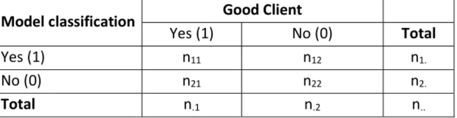
The most common measures of prediction accuracy are computed based on a 2x2 contingence table (e.g., Linden, 2006). A generalization of the contingency table (Table 1) for our study follows, where n11 is the true positive frequency, n12 is the false positive frequency, n21 is the false negative frequency,

and n22 is the true negative frequency.

Model classification Good Client

Yes (1) No (0) Total

Yes (1) n11 n12 n1.

No (0) n21 n22 n2.

Total n.1 n.2 n..

Table 1: Contingence Table

Sensitivity is defined as the proportion of true positives that were correctly predicted by the model as being a "Good Client”, thus it is given by

. . Specificity is defined as the proportion of true negatives

that were correctly predicted by the model as not being "Good Client", and it is given by

. . The ROC

curve shows the trade-off between Sensitivity and Specificity (an increase in Sensitivity will imply a decrease in Specificity). False-negatives (FN) are defined as the proportion of "Good Clients" not predicted as such by the model:

. . False-positives (FP) are defined as the proportion of clients who

are not "Good Clients" but categorized as such by the model:

. . The percentage of correctly classified

individuals is given by

.. × 100.

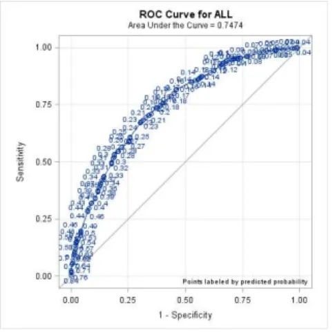
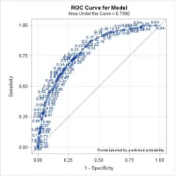
The ROC curve is a graph of Sensitivity (or true positive rate) versus false positive rate, i.e. it represents the Sensitivity (ordinates) versus 1 – Specificity (abscissa) resulting from the variation of a cut-off value along the axis of decision x. Thus, the representation of the ROC curve allows to show the values for which there is optimization of Sensitivity as a function of Specificity, corresponding to the point that is closest to the upper left corner of the diagram, since the positive sign is 1 and the of false positive 0. The area below the ROC curve gives us a measure of discrimination, which indicates to us the possibility of a “Bad” client having an associated estimated probability higher than a “Good” client.

17 In the graphic of the ROC curve, the diagonal line (x=y) indicates that model predictions are no better than random guesses. The further the points are above the diagonal line, the better the predictive accuracy of the model. Let R be the value corresponding to the area below the ROC curve, and as a general rule we have the following guidelines (Ekelund, 2012):

 If R = 0,5 then there is no discrimination;  If 0,6 < R < 0.7 then the discrimination is poor;  If 0,7 < R < 0.8 then the discrimination is fair;  If 0,8 < R < 0,9 then there is a good discrimination;  If R ≥ 0,9 then there is a very good discrimination.

18

4.

RESULTS AND DISCUSSION

Firstly, a descriptive analysis of some variables will be made. Next, we will do a discriminant univariate analysis, where we will select the variables that will have a good behaviour when they are alone as the only independent variable in the model. After it, with those variables a regression model will be investigated and the best variables for the multivariate model will be discovered. To prove that the model is appropriate we will test correlations between independent variables. Finally, the coefficients interpretation will be made, and some diagnosis analyses will be applied to the model to assess its goodness of fit and performance.

4.1

D

A

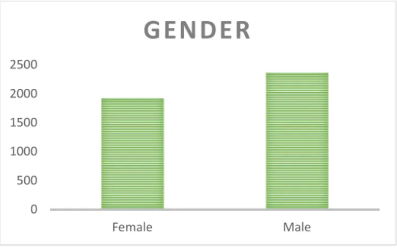
In this section we will describe the main dataset in general characteristcs. Firstly, the population is composed by 1920 Female clients and 2364 Male clients which corresponds to 45% of women vs 55% of men (Figure 1).

Figure 1: Distribution of sample individuals by gender

Regarding with the Marital Status we have: 1660 married; 627 divorced; 87 separated; 1323 single; 394 Non-marital partnership; 193 widowed (Figure 2).

Figure 2: Distribution of sample individuals by marital status

The following graphic represents the age distribution in the main dataset. The age range between 40 and 43 has the highest frequency of credit cards holders (Figure 3).

0 500 1000 1500 2000 2500 Female Male

GENDER

MARITAL STATUS

19

Figure 3: Distribution of sample individuals by age

The next variable is payment method, as we can see most of our clients prefer not fixed payment at the end of the month (2891 clients - 68% of individuals) versus fixed payment (1393 clients - 32% of individuals) (Figure 4). The not fixed payment method is the one that give the company proftability because is the one that clients pay some interests to the company.

Figure 4: Distribution of sample individuals by payment method

In terms of postcode we can say that most of the 4284 clients live almost in the centre or in the north of Portugal but also exists some that live in the south. As it was said by Arriaga, 2013, most credit card holders are males. As it was mentioned by Arriaga (2013) when men are married, they hold more credit cards. In the company concerned, the range between 40 and 43 hold more credit cards. Fact that is against the conclusions of Arriaga (2013) who said that that range is the age between 26 and 35 years old.

4.2

D

U

A

Firstly, with a SAS code, the independent variables (discrete, continuos or category) were transformed in the best dummy agregation possible. The continuous and discrete varibles were transformed in intervals of values and the classificatory variables were agregated in larger groups of classification. This

0 500 1000 1500 2000 2500 3000 3500 Changeable Fixed

PAYMENT METHOD

20 code also gave the Gini coefficient for each best agregation per variable and with it the best variables (variables with Gini greater than 10) were selected. The result was 11 discriminant variables:

 PostCode;  Plafond;  Encours;  CRCCredit;  FinancingAmountMonth;  Job;  Ifee;  OpeningAmount;  FinancingSeniority;  ClientSeniority;  UtilizationTax.

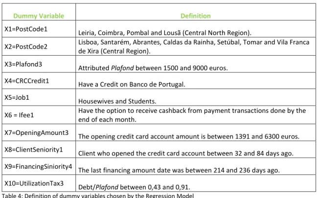
A discriminant variable is a variable that is good alone in the model. This was a hint to build the regression model. The starting point was all 73 variables but the variables included on the regression model were the ones that have good Gini values in this discriminant analysis. The Gini value is a measure of statistical dispersion.The following table (Table 2) shows all the dummies generated from the discriminant variables:

Dummy Variable Definition (where dummy variable=1) PostCode1 Leiria, Coimbra, Pombal and Lousã (Central North Region).

PostCode2 Lisboa, Santarém, Abrantes, Caldas da Rainha, Setúbal, Tomar and Vila Franca de Xira (Central Region).

PostCode3 Algarve and Alentejo (South Region). PostCode4 Aveiro, Guimarães and Porto (North Region). Plafond1 Attributed Plafond between 500 and 750 euros. Plafond2 Attributed Plafond between 1000 and 1250 euros. Plafond3 Attributed Plafond between 1500 and 9000 euros. Encours1 Debt to the company between 0 and 664 euros. Encours2 Debt to the company between 665 and 1528 euros. Encours3 Debt to the company between 1529 and 8207 euros. CRCCredit Have a credit on Banco de Portugal.

FinancingAmontMonth1 Average financing amount at the end of the month zero euros.

FinancingAmountMonth2 Average financing amount at the end of the month between 1 and 60 euros. FinancingAmountMonth3 Average financing amount at the end of the month between 61 and 1425 euros FinancingAmountMonth4 Average financing amount at the end of the month greater than 1426 euros.

Job1 Housewives and Students.

Job2 Receptionists, Telephone Operators, Unemployed, people from Army, Navy, Air _{Force, Tourists Guides and Hostesses.} Job3 Real Estate Agents, Stock Brokers, Commercial Representatives, Typists, _{Stenographers, Financial Services and Accounting Employees.}

Job4 Biologists, Botanists, Zoologists, Doctors, Pharmacists, Veterinarians, Teachers of, Pre-Primary, Engineers, Researchers, Physicists and Astronomers.

Ifee1 Have the option to receive cashback from payment transactions done by the end of _{each month.} OpeningAmount1 The opening credit card account amount is zero.

OpeningAmount2 The opening credit card account amount is between 1 and 1390.

OpeningAmount3 The opening credit card account amount is between 1391and 6300 euros. ClientSeniority1 Client who opened the credit card account between 32 and 84 days ago.

21 Dummy Variable Definition (where dummy variable=1)

ClientSeniority2 Client who opened the credit card account between 85 and 215 days ago. ClientSeniority3 Client who opened the credit card account between 216 and 363 days ago. FinancingSiniority1 Didn't do any financing.

FinancingSiniority2 The last financing amount date was between 3 and 64 days ago. FinancingSiniority3 The last financing amount date was between 65 and 213 days ago. FinancingSiniority4 The last financing amount date was between 214 and 236 days ago. FinancingSiniority5 The last financing amount date was between 237 and 362 days ago. UtilizationTax1 Debt/Plafond between 0 and 0,18.

UtilizationTax2 Debt/Plafond between 0,19 and 0,42. UtilizationTax3 Debt/Plafond between 0,43 and 0,91. UtilizationTax4 Debt/Plafond between 0,92 and 1,45. UtilizationTax5 Debt/Plafond between 1,46 and 12,87.

Table 2: Definition of dummy variables

4.3

L

R

-

M

A

After the discriminant univariate analysis, the selection of variables for the multivariate model will start. The significance level chosen was the default one, 0,05. Meaning that in the stepwise selection, when p-value is greater than or equal to 0,05 the variable will be rejected from the model, and when p-value is less than 0,05 the variables will become part of the model. From those 11 discriminat variables which correspond to 36 dummy variables, the stepwise procedure selected 10 dummies used in the final model (Table 3). The type os variables that originated those 10 dummy variables are showed in Appendix 1.

Variable Gini Concordance

PostCode1 11,4% 14,7% PostCode2 31,2% 46% ClientSiniority1 36,1% 55,6% Plafond3 41,4% 64,3% OpeningAmount3 44,7% 67,3% CRCCredit1 47,5% 71,3% Ifee1 48,6% 72,5% Job1 48,8% 72,7% UtilizationTax3 49,7% 73,6% FinancingSiniority4 50% 73,9%

Table 3: Stepwise Selection variables

The model obtained with those dummies was: y = – 2,94239637 + 1,9806062086X1 + 0,9549803878X2 + 0,8213695288X3 – 0,5528866225X4 + 2,7747835357X5 + 0,4412305184X6 – 1,413281874X7 + 0,7228322149X8 – 0,328989972X9 – 0,257071131X10

Where, X1=PostCode1; X2=PostCode2; X3=Plafond3; X4=CRCCredit1; X5=Job1; X6=ifee1; X7=OpeningAmount3; X8=ClientSeniority1; X9=FinancingSeniority4; X10=UtilizationTax3.

22

Dummy Variable Definition

X1=PostCode1 _{Leiria, Coimbra, Pombal and Lousã (Central North Region).}

X2=PostCode2 Lisboa, Santarém, Abrantes, Caldas da Rainha, Setúbal, Tomar and Vila Franca _{de Xira (Central Region).} X3=Plafond3 _{Attributed Plafond between 1500 and 9000 euros.}

X4=CRCCredit1 _{Have a Credit on Banco de Portugal.} X5=Job1 _{Housewives and Students.}

X6 = Ifee1 Have the option to receive cashback from payment transactions done by the _{end of each month.} X7=OpeningAmount3 The opening credit card account amount is between 1391 and 6300 euros. X8=ClientSeniority1 _{Client who opened the credit card account between 32 and 84 days ago.} X9=FinancingSiniority4 The last financing amount date was between 214 and 236 days ago. X10=UtilizationTax3 _{Debt/Plafond between 0,43 and 0,91.}

Table 4: Definition of dummy variables chosen by the Regression Model

Observing the output of SAS (Table 3 and Table 4) we can highlight:

- The p-value of the Likelihood Ratio test is smaller than 0,05 (Table 5), so we reject the null hypothesis. Therefore, there is evidence that at least one of the predictors’ regression coefficient is not equal to zero in the model.

- The global Score and Wald tests provide the same conclusion as the Likelihood Ratio test (Table 5): there is evidence that at least one of the βi (coefficient of each variable) is different from

zero, because we reject the same null hypothesis.

Test _Square Chi- DF p-value

Likelihood Ratio 605,99 10 <0,0001

Score 588,8739 10 <0,0001

Wald 489,8291 10 <0,0001

Table 5: Results of Likelihood ratio test, Score test and Wald test

- The Wald test for each parameter (Table 6) allows to conclude that all coefficients of the selected dummies are significantly different from zero. The dummies that were not selected for the model have the p-values of this test above the significant level of 0,05.

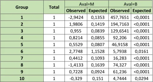
23 Parameter DF Estimate Standard _Error Wald Chi-Square p-value

Intercept 1 -2,9424 0,1353 457,7651 <0,0001 PostCode1 1 1,9806 0,1419 194,7163 <0,0001 PostCode2 1 0,955 0,0839 129,6541 <0,0001 Plafond3 1 0,8214 0,0855 92,206 <0,0001 CRCCredit1 1 0,5529 0,0807 46,9158 <0,0001 Job1 1 2,7748 1,1528 5,7938 0,0161 ifee1 1 0,4412 0,1093 16,283 <0,0001 OpeningAmount3 1 -1,4133 0,1639 74,327 <0,0001 ClientSiniority1 1 0,7228 0,0924 61,236 <0,0001 FinancingSeniority4 1 -0,329 0,151 4,7444 0,0294 UtilizationTax3 1 -0,2571 0,091 7,9848 0,0047

Table 6: Analysis of Maximum Liklihood Estimates

4.4

M

A

A Correlation Analysis was developed between those selected variables: there should be no high correlations among the independent variables.

The following table (Table 7) shows the results of the Pearson Chi-Square test applied to all pairs of 10 dummy variables selected for the model. All p-values are above 0,01, so we do not reject the null hypothsis for any test. Therefore, there is no significant relationship between each pair of variables.

Table 7: P-values of the Pearson Chi-Square test applied to the variables of the Regression Model

Pearson Correlation P-Value

PostCode1 PostCode2 Plafond3 CRCCredit1 Job1 Ifee1 OpeningAmount3 ClientSeniority1 FinancingSiniority4 UtilizationTax3

PostCode1 - - 0,7963 0,0353 0,5579 0,0807 0,2062 0,0241 0,8901 0,3813 PostCode2 - - 0,017 0,0595 0,9361 0,02 0,8797 0,022 0,4094 0,0255 Plafond3 0,7963 0,017 - 0,4434 0,8947 0,023 0,02 0,022 0,0184 0,02 CRCCredit1 0,0353 0,0595 0,4434 - 0,7095 0,4793 0,0576 0,7026 0,0206 0,02 Job1 0,5579 0,9361 0,8947 0,7095 - 0,2289 0,4214 0,2475 0,4597 0,4619 Ifee1 0,0807 0,02 0,023 0,4793 0,2289 - 0,023 0,02 0,7779 0,025 OpeningAmount3 0,2062 0,8797 0,02 0,0576 0,4214 0,023 - 0,5958 0,02 0,3472 ClientSeniority1 0,0241 0,022 0,022 0,7026 0,2475 0,02 0,5958 - 0,023 0,03 FinancingSiniority4 0,8901 0,4094 0,0184 0,0206 0,4597 0,7779 0,02 0,023 - 0,021 UtilizationTax3 0,3813 0,0255 0,02 0,02 0,4619 0,025 0,3472 0,03 0,021 -

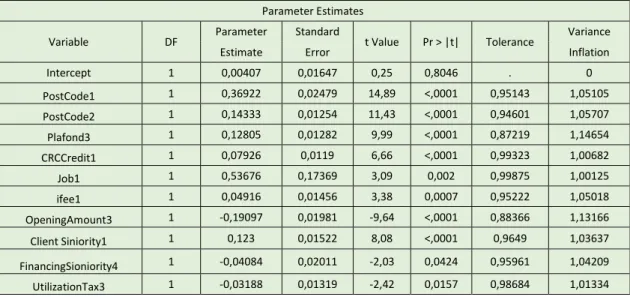
24 A collinearity statistics analysis was done and the results are presented in Table 8. Hence those results indicate that there is no problems of multicollinearity since all VIF values are smaller than 10 and even bellow the value 2,5.

Table 8: Collinearity Statistics

Another collinearity diagnosis was done based on the Condition Index, and Table 9 shows those results. Those values indicate that there is not problems of collinearity because none of the Condition Indexes are above 30 or even greater than 15.

Table 9: Collinearity Diagnosis

Parameter Estimates

Variable DF Parameter Standard t Value Pr > |t| Tolerance Variance

Estimate Error Inflation

Intercept 1 0,00407 0,01647 0,25 0,8046 . 0 PostCode1 1 0,36922 0,02479 14,89 <,0001 0,95143 1,05105 PostCode2 1 0,14333 0,01254 11,43 <,0001 0,94601 1,05707 Plafond3 1 0,12805 0,01282 9,99 <,0001 0,87219 1,14654 CRCCredit1 1 0,07926 0,0119 6,66 <,0001 0,99323 1,00682 Job1 1 0,53676 0,17369 3,09 0,002 0,99875 1,00125 ifee1 1 0,04916 0,01456 3,38 0,0007 0,95222 1,05018 OpeningAmount3 1 -0,19097 0,01981 -9,64 <,0001 0,88366 1,13166 Client Siniority1 1 0,123 0,01522 8,08 <,0001 0,9649 1,03637 FinancingSioniority4 1 -0,04084 0,02011 -2,03 0,0424 0,95961 1,04209 UtilizationTax3 1 -0,03188 0,01319 -2,42 0,0157 0,98684 1,01334 Collinearity Diagnostics Number Eigen _value Conditio_{n Index}

Proportion of Variation Intercept _Post

Code1 Code2 Post Plafond3 Credit1 CRC Job1 ifee1

Opening Amount

3 Siniority1 Client Sioniority4 Financing Utilization Tax3

1 4,444₂₈ 1 0,00588 0,00355 0,01389 0,013 0,01448 0,00011₅₆₆ 0,00853 0,0078 0,01043 0,00542 0,01213 2 1,024₂₅ 2,08304 0,0000201₂ 0,10523 0,00182 0,00070₅₉₂ 0,000277 0,01028 0,00033₁₂₄ 0,07711 0,19236 0,41368 0,01055 3 1,007₉₃ 2,09984 0,0000032₁ 0,34747 0,03696 0,00006₄₉₇ 0,000497 0,50537 0,00000₂₂₇ 0,00321 0,00483 0,01384 0,0031 4 0,994₃₄ 2,11414 0,0000022₁ 0,30009 0,03744 0,00075₈₃₄ 0,00107 0,45371 0,00002₇₉₆ 0,00604 0,01527 0,09733 0,00363 5 0,885₈₈ 2,23982 0,00128 0,00417 0,02628 0,01942 0,00812 0,02685 0,00418 0,64073 0,00884 0,08188 0,02037 6 0,752₈₂ 2,42971 0,0000625₆ 0,00102 0,01855 0,00187 0,00272 0,00095₂₂₇ 0,00055₆₄ 0,00304 0,29801 0,06898 0,57226 7 0,624₀₆ 2,66862 0,0009567₆ 0,02491 0,10328 0,01358 0,04184 0,00208 0,00749 0,00784 0,43907 0,26451 0,24472 8 0,493₂₈ 3,00162 0,00137 0,16552 0,54663 0,00324 0,39486 0,00026₄₅₆ 0,0023 0,01278 4,29E-07 0,01537 0,01287 9 0,424₃₃ 3,23632 0,0047 0,03171 0,14332 0,2973 0,36684 0,00019₄₉₉ 0,06119 0,10721 0,00443 0,000592 0,03582 10 0,254₁₉ 4,18143 0,03497 0,00963 0,0442 0,61897 0,07454 0,00001₉₇₈ 0,33084 0,12777 0,01612 0,02221 0,00728 11 0,094₆₄ 6,85269 0,95075 0,00