Control of Incident Shock-Induced Separation Using
Vane-Type Vortex-Generating Devices
S. B. Verma∗and C. Manisankar†
National Aerospace Laboratories, Bangalore 560 017, India DOI: 10.2514/1.J056460
An experimental investigation was conducted to control an incident shock-induced boundary-layer separation associated with a 14 deg shock generator in a Mach 2.05 flow. Two vane-type configurations, namely the triangular (h∕δ0.3, 0.5, 0.8, 1.0) and the rectangular (h∕δ0.5) designs, were studied. An array of each control device was tested for three control locations ofX∕δ5, 10, and 15. The control location of5δis seen to show the maximum reduction in separation length for each device tested. For the rectangular-vane device (h∕δ0.5), a maximum reduction of 38% in separation length is observed, followed by the triangular-vane devices ofh∕δ0.8and 1.0, each of which shows a 32% reduction, and finally,h∕δ0.5with 18%. The effectiveness of these devices to control separation is, however, seen to decrease with increase in X∕δ. In terms of separation shock unsteadiness, the maximum rms value forX∕δ5δshows the highest value for each control device, and this value decreases with increase in control location. AtX∕δ15, both the rectangular vane (h∕δ0.5) and triangular vane (h∕δ0.8;1.0) show a 50% reduction in maximum rms value, whereas it decreases to 30% atX∕δ10for these devices.
Nomenclature
F = fluctuation frequency, Hz
Gf = power spectral density,kPa2∕Hz g = shock generator exit height, mm h = height of the control device, mm L = length of the flat plate model, mm Pw = local mean wall pressure, kPa P0 = tunnel stagnation pressure, kPa p∞ = freestream static pressure, kPa
q∞ = freestream dynamic pressure, kPa
Rpp = space-time cross-correlation function s = center-to-center interdevice spacing, mm U∞ = freestream velocity, m/s
w = shock generator wedge length, mm
X = coordinate along model centerline, mm XIL = interaction length (Ximp−Xs) from schlieren
images, mm
Ximp = impact point location of incident shock, mm XSL = separation length (Ximp−Xsep) with respect to
impact point location, mm
Xs = impact point location of separation shock, mm Xsep = first rise in wall pressure along the centerline,
mm
X2pl = first point of wall pressure that reaches the second pressure plateau, mm
α = angle of incidence of the control device vanes, deg
ΔXC = reduction in the separation bubble length with control, mm
ΔXNC = separation bubble length for no control (X2pl−Xsep), mm
δ = boundary-layer thickness, mm
δ = boundary-layer displacement thickness, mm
θ = boundary-layer momentum thickness, mm
ξ = separation distance for which the correlation was performed, mm σw = Pn i0Pwi−Pw − 2 ∕n−1 q , standard devi-ation or rms of wall pressure fluctudevi-ation, kPa
σw∕Pw = nondimensionalized local value of rms σw∕Pwmax = nondimensionalized maximum value of rms
I. Introduction
S
HOCK-WAVE/BOUNDARY-LAYER interactions (SWBLIs) are fundamental to the design of any supersonic air intake wherein the process of flow deceleration occurs through a complex system of shocks. However, under certain operating conditions, the interactions may cause large areas of separated flow, which then presents itself as an aerodynamics obstruction to the oncoming flow (Fig. 1). This can significantly alter the flow deceleration process and, in the worst-case scenario, can also result in an engine unstart condition. Another matter of concern associated with such interactions is the large-amplitude fluctuating pressures accompanying the shock oscillations [1–5] that can be detrimental to the structural integrity of the vehicle components [1]. The major challenge, therefore, lies in implementing effective flow control strategies upstream of such interactions to improve the health of the incoming boundary layer so as to avoid or reduce the extent of separation and the associated flow unsteadiness and, hence, improve the intake performance over the flight envelop.The most commonly adopted flow control strategy is that of boundary-layer manipulation [6,7]. The method relies on increasing the boundary-layer momentum before its interaction. By doing so, the reenergized boundary layer is able to sustain relatively higher adverse pressure gradients that help to delay as well as reduce the extent of separation. There are several ways suggested in the literature to achieve this. The first and foremost technique is by the use of surface suction or bleed ahead of the interaction [8–11]. The method involves the removal of a significant amount of boundary-layer mass flow (of the order of 2–5% of intake mass flow) [10–12], resulting in a newer and much thinner boundary layer that is more resistant to separation. The capability of this control technique is indisputable and has hence found many hardware applications. The technique, however, comes with several performance penalties, such as increase in inlet area to compensate for the mass flow removal leading to an increase in ram drag [12,13], system complexity, and the associated increase in gross takeoff weight. With these issues in mind, efforts were channeled to develop an alternate control strategy that could achieve similar benefits of separation control as that of bleed but would avoid losses associated with mass flow removal while maintaining the intake performance [12,13]. From this perspective, the use of a vortex generator (VG) Received 22 June 2017; revision received 17 November 2017; accepted for
publication 12 December 2017; published online 23 January 2018. Copyright © 2017 by the authors. Published by the American Institute of Aeronautics and Astronautics, Inc., with permission. All requests for copying and permission to reprint should be submitted to CCC at www.copyright.com; employ the ISSN 0001-1452 (print) or 1533-385X (online) to initiate your request. See also AIAA Rights and Permissions www.aiaa.org/randp.
*Deputy Head, Experimental Aerodynamics Division, Council of Scientific and Industrial Research; [email protected]. Associate Fellow AIAA.
†Senior Scientist, Experimental Aerodynamics Division, Council of Scientific and Industrial Research; [email protected].
1600 Vol. 56, No. 4, April 2018
placed upstream of the interaction provides a promising control alternative wherein the exchange of momentum from the freestream to the near-wall flow regions is now provided by a pair of counter-rotating vortices (CRVs) resulting in a relatively fuller and more stable boundary layer [14,15]. Various types of VG devices, both active or passive, have been tested in the literature. The active approach uses plasma jets [16–18] or steady [19–23] or pulsed micro air jets [18,24] (normal or angled to the main flow), which (on interaction with the oncoming flow) generate streamwise vortices. Although the active control has the added advantage of being switched on or off as per requirement [19,20], they do require input of extra energy for their activation and, hence, may increase installation and maintenance costs. The passive approach, on the other hand, uses fixed mechanical devices projecting into the boundary layer, such as vanes in co- or counter-rotating configuration, microramps, etc., to initiate a similar effect. Verma and Hadjadj [25] give a detailed comprehensive view of the various flow control techniques used in SWBLIs. Although the active control has the added advantage of being switched on or off as per requirement [19,20], they do require input of extra energy for their activation and, hence, may increase installation and maintenance costs. From this perspective, a mechanical VG is preferable. However, the device drag in their case is unavoidable, especially when they are not needed. The fact is true, however, more for traditional VGs (h∕δ≥1), which can slightly offset their benefits [14]. As a result, sub-boundary-layer vortex generators orh∕δ≤0.6with relatively much lesser drag penalty were suggested [26,27] and found to be quite effective in separation control. But because of their small size, these control devices need to be placed much closer to the region of interaction, as opposed to the traditional VGs [28], for maximum benefit. The important parameters that control a flow interaction are the device height with respect to the boundary-layer thickness (h∕δ), the spanwise spacing (s∕h) between the VGs, and the location of implementation of these devices (X∕δ) with respect to the interaction location [29,30]. Various mechanical VG configurations, such as the microramps [28–47], split ramps [27,33,36,39,40], and ramp-vane designs [36–40,46–48], have been tested in the literature. Computa-tional studies conducted in the recent past [39–41,48] have revealed that the general flow features and the momentum flux added to the near-wall region [39,40,48] scale linearly with device height, indicating that a larger-sized control device is more effective in stabilizing the interaction.
Most of the previously reported studies, both computational [39,40,48] and experimental [37,38], which have made a comparative assessment of various micro-VG configurations in controlling an interaction, were primarily in the transonic flow regime. Experimental [29,30,35,36,42] and computational [34,39,43,44] studies in supersonic interactions have also been reported, but these are mostly using microramps of Anderson configuration and not comparative studies. Out of these, the study by Anderson et al. [34], however, does report the use of various micro-VG devices in a Mach 2 incident shock-induced separation. However, they do not indicate the impact of each VG design on the extent of separation nor on the separation shock unsteadiness. More recently, an assessment of various VG configurations has been reported in a Mach 2 incident shock-induced
separation for separation control [46,47]. However, other than the popularly studied ramp-vane or triangular-vane devices, none of the studies in the supersonic regime report the use of rectangular vanes in controlling separation. The primary objective of the present study was, therefore, to investigate and compare the effect of 1) vane shape, such as triangular (h∕δ0.3, 0.5, 0.8 and 1.0) and rectangular (h∕δ0.5) configurations, and 2) variation in their control distanceX∕δfrom separation location relative to no control, in effectively controlling separation and separation shock unsteadiness. Here,δis the boundary-layer thickness upstream of separation, discussed in Sec. II.A. The only studies that report such a comparison are by Shim et al. [49] and Velte et al. [50], but both of these studies have been conducted in the incompressible range (10 m∕s). To the best of the authors’knowledge, such a study in supersonic interactions is unavailable in the literature.
II. Experimental Setup and Procedure A. Wind-Tunnel Facility and Model Details
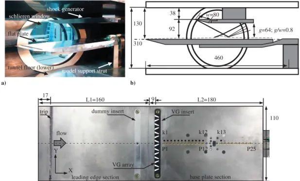
Experiments were performed in the 0.46×0.3 m blowdown trisonic wind-tunnel at National Aerospace Laboratories (NAL). All tests were conducted at a freestream Mach number of2.050.02 (U∞523 m⋅s−1) and a unit Reynolds number Re∕L of 25.257×10⁶m−1. The wind-tunnel stagnation pressure P0 and temperatureT0were208.5 kPa2%(absolute) and298 K0.4%, respectively. The wall temperature was assumed adiabatic, and the turbulence levels in the tunnel were approximately 0.2% (%Cprms). A 14 deg wedge of 0.22 m width and lengthw0.08 mwas mounted on the tunnel top wall to generate a shock wave (β42.93 deg) that impinges on a sting-mounted flat-plate model along the tunnel centerline, as shown in Figs. 1a and 1b. The flat plate was 0.34 m long with a span of 0.11 m (Fig. 1c). The Reynolds numberRexbased on the entire flat-plate length was8.58×106. To ensure a turbulent boundary layer, a trip made of 60 grit carborundum particles spanning the plate width and 4 mm in length was placed 17 mm from the leading edge. A total of 25 mean pressure port locations (P1 to P25) are available along the plate centerline to capture the entire interaction. For unsteady pressure measurements, 13 Kulite pressure transducers have been provided, but the pressure sensing ports were located 5 mm off the centerline, as shown in Fig. 2c. As a consequence of the latter, rms values are available only for these locations (results discussed in Sec. III.C). This measurement location also corresponds to a device off-center location of almost 100% span.
For the present test setup, ag∕wvalue of 0.8 (Fig. 2b) was selected so as to ensure that the expansion fan emanating from the downstream end of the wedge did not interact with the incident shock to influence the interaction in any way, as seen in Fig. 3a. Here,gis the shock generator exit height, as shown in Fig. 2b. Based on inviscid calculations, the distance of the incident shock impingement location (long dashed line) and the first characteristic of the expansion fan (short dashed line, Fig. 3a) was approximately6δ. This is seen as a second pressure plateau in the wall pressure distribution in the region of maximum pressure (Fig. 3b). The inviscid pressure ratio for this interaction is 3.2. The interaction lengthXIL, defined as the distance between extrapolated wall impact points of incident (Ximp) and separation/reflected shocks (Xs) as evaluated from the schlieren images, and the separation lengthXSL, the distance between the first rise in wall pressure (Xinc) along the centerline andXimp, are371 and411 mm, respectively, for the no-control case. Despite the variation in their spanwise locations, the Kulite and electronic pressure scanner (ESP) pressure distributions overlap and show the surface pressure rise across the interaction to be very uniform on either side of the centerline, indicating a straight separation line on either side of the model centerline, as is also seen and discussed in surface oil pictures in Sec. III.C. However, owing to the finite spanwise extent of the flat plate, three-dimensional effects do begin to influence the interaction toward the outer edges of the flat plate. It may, therefore, be borne in mind that the discussion of the results in this paper are limited only to that finite region of the flow about the centerline where the separation line is seen to be straight for no control. No side fences were used on the plate to facilitate schlieren imaging.
undisturbed b’layer
incident shock
separation shock
reflected shock expansion fan
recirculation zone reattachment
shock sonic line
Ximp
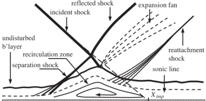
Fig. 1 Schematic showing the important flow features of incident shock-wave/boundary-layer interaction phenomena with boundary-layer separation.
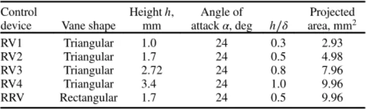
Control devices of two vane-type configurations, namely triangular or ramped vane (RV) [29,39,40,46,47] and rectangular vane [49,50], were tested to compare the capability of each of these to control the flow interaction. Each of these devices was arranged in the form of an array in a single row. The array was made in such a way that one VG device of each configuration was always placed on the model centerline and in line with streamwise row of the mean pressure measurement locations P1 to P25. Figure 4 shows the schematic of the two vane-type configurations used in the present study, and Table 1 shows the designations used in the present paper
based on its configuration, height, and the associated projected area for each device pair. The angle of incidence α for both the VG configurations is 24 deg (Fig. 3). An interdevice spacing ofs 12 mm(center-to-center) and an intervane (or trailing-edge) spacing of1his maintained for all device heights, resulting in an array of seven control devices for each configuration. Although the triangular vane was studied for various device heightsh∕δ0.3, 0.5, 0.8, and 1.0, the rectangular vane device was, however, tested for only h∕δ0.5. To further investigate the most effective location for implementation of separation control, an array of each control -1.6 -1.2 -0.8 -0.4 0.0 0.4 0.8 1.0 expansion fan separation bubble incident shock re-attachment shock reflected shock separation shock a) (X-Ximp) / XIL Pw /P∝ -1.6 -1.2 -0.8 -0.4 0 0.4 0.8 1.2 1.6 2 0.5 1 1.5 2 2.5 3 3.5 centreline Y=5mm inviscid 1stpressure plateau undisturbed boundary layer 2ndpressure plateau K13 K12 b)
Fig. 3 Plot showing a) the schlieren image of the interaction, and b) the associated streamwise mean pressure distribution (no control). a)
flat plate
shock generator
model support strut tunnel floor (lower)
schlieren window b) 460 310 130 92 38 g=64; g/w=0.8 w=80 L1=160 L2=180 flow k1 k12 P1 P12 P25
dummy insert VG insert trip
110
leading edge section base plate section X Y c) 17 9 k13 VG array
Fig. 2 Details of a) the model mounted in the wind-tunnel, b) a schematic of the experimental setup, and c) flat-plate model details with the pressure sensor and VG insert locations. All dimensions are in millimeters.
Z Y X h 1mm α= 24o 1h 7.2mm h=1.75mm 1mm α= 24o 1h 7.2mm a) b)
Fig. 4 Schematics of the vane-type control configurations a) triangular vane (h∕δ0.3, 0.5, 0.8, 1.0), and b) rectangular vane (h∕δ0.5).
configuration was implemented atX5δ,10δ, and15δupstream of the separation location for no control. This was achieved by moving the wedge downstream relative to the flat plate to a predetermined shock impingement location calculated based on the isentropic relations. In terms of impingement locationX−Ximp∕XIL, these distances correspond to −1.6, −1.9, and −2.2, respectively. The boundary-layer thickness just upstream of the separation for no control, as estimated from the schlieren images, was δ3.4 0.06 mm at X∕δ10. For the three X∕δ locations tested, the boundary-layer thickness varied by approximately 0.2 mm, which was seen to have negligible effect on the interaction length (Fig. 5). The boundary-layer thickness was also estimated based on length Reynolds numberRexfor turbulent flows (3.48 mm) with a corrected value of (3.56 mm) for compressible flows as suggested by Van Driest [51]. However, such an estimate may differ from the boundary-layer thickness calculated from velocity profile by 3% [52]. The experimental conditions and the undisturbed boundary-layer properties are shown in Table 2. Here,SeandLcorrespond to the separation criteria and the nondimensional interaction length (value obtained from the best fit line) based on scaling described by Souverein et al. [53]. The mean skin-friction coefficientcf, after correction for turbulent flows [51], is2.1×10−3.
B. Signal Conditioning and Data Acquisition System
The wall static pressures were measured using both ESPs and Kulite transducers. The model had 25 (P1 to P25) mean static pressure ports, which were measured using Pressure Systems ESP-16HD 16-port scanners. These scanners were calibrated in situ using a Druck calibrator model DPI-610. An eight-channel signal conditioner module (SCXI-1520) from National Instruments (NI) is used for acquisition of the analog signals from the pressure scanners. The analog signals are then digitized using a 16-channel 16-bit A/D card (NI 6036) that has a maximum sampling rate of 200,000 samples per second. The present data were acquired at 500 Hz, with 500 samples taken for each port location. This resulted in an averaging time of 1 s. The unsteady wall pressure fluctuations were measured using 13 fast piezoresistive Kulite model XCQ-093 M-screen transducers at locations marked K1 to K13 in Fig. 1c. The presence of the protective screen limits the frequency response of these transducers to 50 kHz. The Kulite transducers have a pressure sensitive area of 0.071 cm and an outer casing diameter of 0.26 cm. The transducers were not flush-mounted on the base plate. Instead, a small orifice (of 0.5 mm length and 0.5 mm diameter) connects the
transducer to the flow. This was primarily done to prevent any damage to the transducer-sensing element from any contaminations in the compressed air supply. This cavity configuration results in an estimated resonance frequency of 68.75 kHz. According to the manufacturer’s specifications, these transducers have a natural frequency of approximately 250 kHz. The sensitivity of the transducers is typically 3–4 mV∕psi. These transducers were calibrated statically. The transducer data were acquired using a truly simultaneous acquisition card, the NI 4495 dc series (with 24-bit resolution) at a sampling frequency of 50 kHz. Each sensor was powered by dc power supply, and the signal was passed through an amplifier and a signal conditioner. A low-pass filter of 20 kHz was applied postacquisition during data processing. It may be pointed out here that the present arrangement of keeping the transducers in a cavity does result in a time lag of the order of 1μs in the measurements. This issue, however, is not seen to be problematic because the data are acquired at 50 kHz and later filtered at 20 kHz. For each transducer channel, 200 records of 4096 were acquired, yielding a total of 819,200 data points per channel per tunnel run. For spectral analysis, a 4096-point narrowband fast Fourier transform was performed and later averaged for 200 records, giving a frequency resolution of 12.2 Hz. Schlieren images of the interaction were captured using a Z-type schlieren setup with a vertical knife arrangement. Palflash 501, with spark duration of100μsand pulse energy of 6 J, was used as the light source. The setup uses 3.0-m-focal-length spherical mirrors to collimate and refocus the illumination source at the knife-edge location. Schlieren images were captured using Nikon D1x digital camera (three frames per second) with a 300 mm lens. The exposure time was set at125μs.
The tunnel stagnation pressurePowas acquired using a Druck 4010 series pressure transducer of 1379 kPa range with0.1%of full-scale accuracy, whereas the static pressure measurements such as pw and p∞ were acquired using ESP of 206.8 kPa range with 0.04% of full-scale accuracy. The pressure transducers were calibrated using a five-point calibration procedure before the beginning of the experiments. Further, a single-point check calibration was performed each day to check for any drift in error. The uncertainties in the pressure measurements were estimated using a statistical approach based on repeatability tests. The estimated uncertainty in measurement of total pressure was1.4 kPa, and that for static pressure measurements was 0.7 kPa. The Kulite transducers (170 kPa range) for unsteady pressure measurements were calibrated statically, and the uncertainty obtained from calibration was found to be within1%of full scale. However, in the intermittent region of separation that is associated with high levels of flow unsteadiness, the average pressure uncertainty is likely to be somewhat greater. The repeatability of the peak rms values in the interaction region was found to be roughly within0.04 kPa.
III. Results and Discussions A. Incoming Boundary Layer
The mean wall pressurePwfor the incoming boundary layer was 26.470.7 kPa, and the rms (σw) of the wall pressure fluctuations upstream of the interaction normalized by the freestream dynamic pressureq∞for the present tests was2.18×10−3. In terms ofσ
w∕Pw, Table 1 Details of the projected area for each control device pair
Control
device Vane shape
Heighth, mm Angle of attackα, deg h∕δ Projected area,mm2 RV1 Triangular 1.0 24 0.3 2.93 RV2 Triangular 1.7 24 0.5 4.98 RV3 Triangular 2.72 24 0.8 7.96 RV4 Triangular 3.4 24 1.0 9.96 RRV Rectangular 1.7 24 0.5 9.96
Table 2 Flow characteristics of undisturbed boundary layer
Parameter Quantity
Boundary-layer thicknessδ 3.4 mm Displacement thicknessδ 1.15 mm
Momentum thicknessθ 0.34 mm
Unit Reynolds numberRe 25.257×10⁶m−1
Reθ 0.86×10⁴
Interaction lengthXIL 33 mm
Separation lengthXSL 45 mm
Separation criteriaSe 1.22
Nondimensional interaction lengthL 2.2 Skin-friction coefficientcf 2.1×10⁻³
Fig. 5 Streamwise distributions of wall pressure for the three streamwise shock impingement locations tested (no control).
it was0.00372%. The present value ofσw∕q∞is shown correlated
well with the data from earlier studies for comparison (Fig. 6a). The value is seen to be approximately 60% of the semi-empirical correlation of Lowson [54] and about 45% of that predicted by Laganelli et al. [55]. The space-time cross-correlationRppof the fluctuating wall pressure with streamwise separation distance were also obtained both for the incoming boundary layer and in the separated region (Fig. 6b). Here,ξis the streamwise distance between the Kulite transducers for which the correlation was performed. As reported earlier [56], the maximum ofRppis observed to decrease with increase in separation distance, and the values seem to agree well with the results of Chyu and Hanly [57] for Mach 2.0 flow for both incoming and separated flows (Fig. 6b). However, the convection velocitiesUccould not be estimated because the usable frequency range is limited by the transducer protective M-screen as well as its mounting arrangement in the model to resolve finer scales. Furthermore, the frequency of the temporal scales of the incoming boundary layer are much higher (U∞∕δ150 kHz) than the filter cutoff frequency (of 20 kHz). Because the pressure fluctuations in the SWBLIs are dominated by relatively low frequencies (less than 1 kHz), this is not considered to be a serious limitation. For the incoming undisturbed boundary layer, the probability density
distributions of the pressure fluctuations were essentially Gaussian, with skewness and kurtosis values equal to 0.03 and 3.02, respectively.
B. Flow Visualization: Schlieren
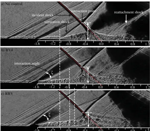
Figures 7 and 8 show the schlieren images of the interaction for control locationsX∕δ5.0and 15, respectively. Only the images for the two best performing control devices, RV4 and RRV, are shown for comparison for each control location. Because of the presence of the dummy inserts and the junction between these two inserts where the leading edge and the base plate sections meet (Fig. 2c), a series of weak waves are seen to emanate into the flow, as seen in Figs. 7a and 8a. Surface oil visualization tests conducted later for no control confirm that these weak disturbances do not introduce any local or spanwise interference in the incoming undisturbed boundary layer that may influence the flow development in any way.
Relative to no control, the presence of the control device upstream of the interaction is seen to introduce some local perturbations: a compression followed by an expansion, and then finally a recompression (Figs. 7b, 7c, 8b, and 8c). The extent of the perturbation introduced is found to increase with increase in device height and is also found to be a function of the device design
a)
∗
M∝ σw /q∝ 1 1.5 2 2.5 3 3.5 4 4.5 5 0 0.002 0.004 0.006 0.008 0.01 0.012 Lawson [54] Laganelli [55] Chu&Hanly [57] Richards et al. [58] Roberts [59] Lewis et al. [60] Dolling & Bogdonoff [61] Present Study∗
b) ξ/δ* Rpp ma x 0 5 10 15 20 0 0.2 0.4 0.6 0.8 1 1.2 1.4Chu & Hanly; M=1.6 [57] Chu & Hanly; M=2, 2.5 [57] Chu and Hanly; M 2.0 Sep. flow [57] Roberts D.R.; M=2.95 [59] Speaker & Ailman; M=3.45 [62] Present Expts: boundary layer Present Expts; sep. flow
Fig. 6 Comparison of the present data with previous studies for a)σw∕q∞and, b) maxima of the space-time correlations in the incoming boundary-layer and separated flow region.
a) No control b) RV4 c) RRV -1.6 -1.2 -0.8 -0.4 0.0 0.4 0.8 1.2 -1.6 -1.2 -0.8 -0.4 0.0 0.4 0.8 1.2 -1.6 -1.2 -0.8 -0.4 0.0 0.4 0.8 1.2 ζ • ζ • separation shock reattachment shock interaction point incident shock interaction angle
Fig. 7 Schlieren images of the interaction with and without control: a) no control, b) RV4, and c) RRV;X∕δ5.0,X−Ximp∕XIL−1.6.
configuration [47]. For example, in case of RV4 and RRV devices, the vane in RV4 design is in the form of a ramp, which reduces the severity of the localized SWBLI in the immediate vicinity ahead of the device (indicated byζ, which is the angle between the compression and recompression shocks) compared to the rectangular-vane RRV. Downstream of these local perturbations, a significant variation in the growth and scale of the flow structures generated from each of these device is seen. Both RV4 and RRV devices are seen to push the separation shock location considerably downstream compared to the no-control case. Compared to the RV4 device, the RRV device is seen to generate structures of much larger scale (marked with dotted lines) immediately downstream of the device, the sizes of which are seen to increase significantly with increase in downstream distance (Figs. 7b, 7c, 8b, and 8c). It has been shown earlier [40] that the size and strength of the vortices shed from a control device increase with increase in device height. In context with the previous result [40], looking at the difference in the scale of the structures shed from RV4 and RRV clearly indicates that much stronger counter-rotating vortices (CRVs) are being shed down-stream of RRV compared to RV4. The reason for this variation in flow development from each of these devices will be discussed in later sections. The impact of relatively stronger CRVs from RRV compared to that from RV4 on the separation shock location is clearly seen forX∕δ5.0(Figs. 7b and 7c), where the RRV device is seen to push the separation shock farther downstream compared to RV4 despite the height of RRV being 50% less than that of the RV4 device. With increase in control location distance, although the device effectiveness is still apparent, the impact of the CRVs on the separation shock location for RV4 and RRV is seen to be almost similar. This could be perhaps due to the phenomena of vortex liftoff, which is known to occur at larger downstream distances (also seen in the schlieren images, Figs. 7c and 8c), hence relatively reducing the ability of the device to control separation. Another apparent effect of the control devices on the interaction is the considerable reduction in the vertical interaction point height (marked by a double headed arrow) with RRV showing maximum reduction. With controls, the reattaching boundary layer no longer seems to be as organized as in the no-control case and is also seen to be much thicker, indicating major changes introduced to the flow structure development with controls.
C. Surface Oil Visualization
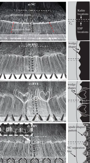
Surface flow topologies with and without control are studied in detail using the conventional surface oil pigment mixture comprising of titanium dioxide powder, vacuum pump oil, and oleic acid. Before a test run, the mixture is carefully sprinkled on the model surface using a toothbrush, which helps to obtain a uniform dot pattern on the area of interest. A good consistency of the oil-pigment mixture ensured that there is no impact of the wind-tunnel shutdown on the oil-flow patterns developed during the runs. The surface oil flow pictures for control locationsX∕δ5.0and 15 obtained after the test runs are shown in Figs. 9 and 10, respectively. The picture on the left for each case shows the surface oil pattern obtained after each test run, whereas the flow topology shown to the right is developed based on the spanwise variations in the flow pattern observed. The black color used in the latter depicts the separation region, whereas the solid white lines in the vicinity of separation have been reproduced from the observed streamline pattern in each case. In the surface oil pictures, a dash-dotted line shown on the model and along the VG centerline represents the mean pressure port locations, and the dashed line marks the Kulite transducer locations. As can be seen, and mentioned earlier, the Kulite transducers are located off-center by 5 mm. For the no-control case, it can be clearly seen that the separation line remains straight for almost 20 mm about the centerline, beyond which it begins to slightly curve downstream (Fig. 9a) and is marked by red dashed lines. It may, therefore, be pointed out that the discussion of the development of flow topology with and without control will be confined only to this region of the interaction where the separation line for no control is observed to be straight about the centerline. It may also be noted that the test model was not removed from the tunnel after each test run for taking pictures of the surface oil pattern. Instead the pictures were taken with one of the tunnel sidewall open and with the camera placed at an angle upstream of the interaction. To assist in accessing the streamline alignment for the no-control cases shown in Figs. 9a and 10a, dotted lines were drawn along the streamwise placed mean pressure ports along the model centerline.
With the introduction of the control devices, significant modifications to the separation line pattern in the form of corrugations are observed (Figs. 9b–9d and 10b–10d). In fact, a b) RV4 a) No control c) RRV -2.4 -2.0 -1.6 -1.2 -0.8 -0.4 0.0 0.4 -2.4 -2.0 -1.6 -1.2 -0.8 -0.4 0.0 0.4 -2.4 -2.0 -1.6 -1.2 -0.8 -0.4 0.0 0.4 ζ • ζ • separation shock reattachment shock interaction point incident shock interaction angle
Fig. 8 Schlieren images of the interaction with and without control: a) no control, b) RV4, and c) RRV;X∕δ15.0,X−Ximp∕XIL−2.2.
significant change is also observed in the flow pattern development with variation in control location and in RV height as well as in device configuration from RV to RRV. A dotted line in each of the flow topologies with control shown in Figs. 9b–9d and 10b–10d marks the no-control separation line for comparison. It has been reported earlier that the size and strength of the vortices generated by the control device are dependent on the height and shape of the device [40], which in turn control the shape and size of the corrugation [47]. The variation in the separation line pattern for each device is indicative of the same. For the RV2 device, the overall separation location is moved downstream compared to no control with the formation of “wedge-shaped”corrugations in the separation line, with each wedge crest in-line with the device centerline (Fig. 9b). For RV1 (h∕δ0.3), the separation line shows a similar pattern but with much smaller corrugations (picture not shown) and no downstream movement of the separation location. Compared to RV2, the separation location for the RV4 device is pushed farther downstream along the model centerline. Two large wedge-shaped corrugations are observed about the model centerline along with a relatively smaller corrugation in between them (Fig. 9c). The streamline pattern behind the large corrugations show a flow pattern resembling a “spade-shaped”formation in the wedge core. A similar pattern was seen for RV3 device also (not shown here). Such a flow topology was not observed for RV devices withh∕δ≤0.5. The RRV device further
shows a significantly pushed-back separation line with individual corrugation patterns resembling well-formed spade shapes, which are seen to be uniformly distributed along the spanwise direction downstream of each device (Fig. 9d). To highlight the observed pattern, a zoom of the surface flow pattern formed at separation is shown on the top left in a box with a dashed boundary. An accompanied effect of this is that almost no spanwise curving of the separation pattern toward the plate outer edges occurs, unlike the no-control and RV test cases. Another interesting feature observed for RRV separation pattern for this location is the prevalence of attached flow conditions in between the adjacent wedge or spade-shaped corrugations and will be discussed later.
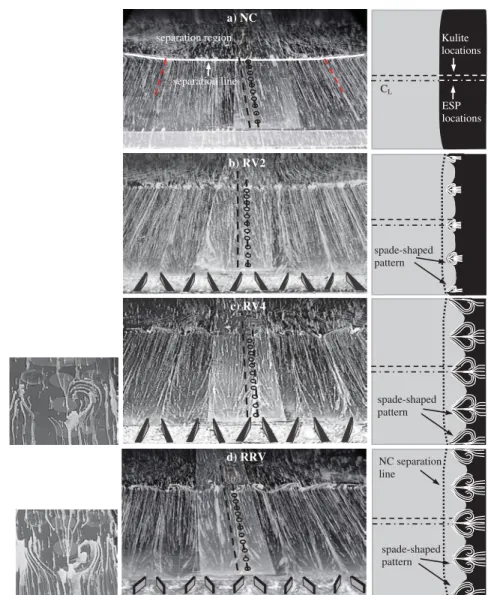
For larger control locations (i.e.,X∕δ15, Fig. 10), the spanwise curving of the separation line in general with controls is observed to almost completely disappear. It is also interesting to see that the corrugations in the separation line are seen to be replaced by spade-shaped patterns at regular spanwise intervals along all the device centerlines and for all control devices. However, the size and shape of each of these is seen to vary. For example, for the RV2 device, the spades are much smaller in size compared to RV3 (not shown) and RV4 (Figs. 10b and 10c), which is expected due to the variation in the CRV size and strength [40] generated from each device. The shape of the spades is also seen to slightly vary in going from RV4 (pointed shape head) to RRV (blunt spade head) due to the configuration change (Figs. 10c and 10d). More on this and the associated physics of flow development from each of these will be discussed in Sec. III.F. D. Streamwise Distribution of Mean Pressure and Standard Deviation
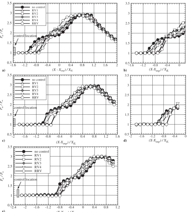
Figure 11 shows a comparison of the streamwise distribution of mean wall pressure with and without control for the three control locations tested. The plots on the left for each control location show the distributions obtained from acquisitions made using ESPs along the model centerline, whereas the plots on the right are from Kulite transducers located 5 mm off the model centerline, as shown in Fig. 2c. For control location 15δ, no meaningful mean pressure distribution is available with Kulite transducers due to the limitation of their location and hence is not shown. The mean pressure distribution forX5δalong the centerline in Fig. 11a clearly shows that, relative to no control, the separation location remains similar for RV1 and is pushed back by two transducer locations for RV2, between two to three locations for RV3 and RV4, and exactly three transducer locations for RRV. Also, the rise in wall pressure at separation location for RRV is seen to continue rising further up to the highest plateau pressure reached at reattachment location (with almost no inflection point) unlike any other control device tested. One interesting feature observed with control and not reported before in literature is the accompanied gradual upstream movement of the reattachment location with increase in RV device height for all control locations (Figs. 11a–11e). Here, the upstream shift in the reattachment point is estimated from the point of intersection of the tangent drawn along the second pressure plateau and that along the rise in wall pressure trend between the two pressure plateaus. This is associated with the accompanied reduction in the interaction point height with control. With RRV, a much higher upstream movement of reattachment location is observed compared to RV3 and RV4 devices especially at 5δ and 10δ control locations. This feature aids in reducing the overall separation bubble length significantly. The mean pressure distribution based on Kulite data in Fig. 11b shows slightly different distributions compared to Fig. 11a, although the overall trends remain almost similar. This was expected because the surface oil pictures clearly indicate significant three-dimensionality introduced at separation location with control. Farther downstream for control location X10δ (Figs. 11c and 11d), although the overall trends in terms of device effectiveness remains the same, the effectiveness of each device in controlling the separation relative to no control is seen to relatively decrease. The latter is seen to further decrease for control locationX15δ(Figs. 11e). With increase in the control location, however, the upstream movement of the reattachment location for each device seems to be unaffected. Kulite locations ESP locations CL d) RRV (c) RV4 b) RV2 a) NC NC separation line spade-shaped pattern wedge shapes wedge shapes c) RV4 separation region separation line
Fig. 9 Surface oil visualization pictures: a) no control, b) RV2, c) RV4, and d) RRV;X5δ,X−Ximp∕XIL−1.6.
Figures 12a and 12b show a comparison of the percentage reduction in separation bubble length (ΔXC∕ΔXNC) with variation in RV device height and a comparison of RV devices with RRV as a function of their control location, respectively. Here, ΔXC is reduction in the separation bubble length defined as the difference in the length between the first rise in wall pressure at separationXsepto the first point of wall pressure that reaches the second pressure plateau (X2pl, reattachment) for control and its value for no control (ΔXNC). A general curve fit has been used to connect the present data. The uncertainty in the estimation of separation bubble length for ΔXNCandΔXC(with control) is about 1.5 and 3%, respectively. This gives a percent error of about 3–4% for the ratioΔXC∕ΔXNCfor the entire range of control configurations and locations. It can be clearly seen that the effectiveness of the RV device in controlling the separation location increases significantly with increase in device height (Fig. 12a), which, as reported by Lee et al. [40], is caused due to increase in the size and strength of the CRVs shed from the larger devices, which in turn is able to transfer the high-momentum air close to the wall much faster, effectively resulting in a more effective control. It is interesting to see that the smallest device RV1 is ineffective in controlling the separation length at all for all control locations. However, as the RV device height is increased to 50% of the incoming boundary-layer thickness (RV2), the effectiveness of the device in controlling the separation begins to show up, with the control location of5δbeing the most effective (18% reduction). A significant reduction in the separation length is further observed for control devices RV3 and RV4 (up to 30% for control location5δ) compared to no control. The effectiveness of these devices, however, decreases with increase in the control location. The results also
indicate that the effectiveness of the RV device seizes beyond0.8δ, after which no change in the separation length is observed for device height 1.0δ. Figure 12b shows a comparison of the percentage reduction in separation length for RV and RRV devices. It is clearly seen that, over the entire range of control locations tested, the RRV devices score well over the RV4 device despite being half of its height. A maximum reduction in separation length of approximately 38% is seen for RRV at control locationX5δ. Compared to RV2, which is of the same height as RRV, the RRV device is able to further reduce the separation length by almost 110%, which is noteworthy. Figures 13a and 13b show the streamwise distribution of rms value for each test case for control locations5δand15δ, respectively. In the intermittent region of separation, the local rms values are seen to rise significantly from their value in the undisturbed boundary layer and tend to reach a peak value after which they begin to drop. In the separated region, following immediately after the intermittent region, the rms values tend to stabilize but still remain much higher than that observed in the undisturbed boundary layer. The maximum rms values are taken from each of these distributions and plotted in Figs. 14a and 14b for RV devices as a function of the height and the control location and for RV4 and RRV as a function of the control location, respectively. Several conclusions can be drawn from these plots. For RV devices, first, it is clearly seen that an increase in the control location helps to decrease the maximum rms value for each device height. Second, for each control location, an increase in device height up to0.5δis seen to increase this value relative to no control. As a result, from the perspective of controlling the shock unsteadiness, an RV device height of0.8δand above is suggested but for control locationsX∕δ≥10. Similarly, for an RRV device, the d) RRV c) RV4 b) RV2 CL Kulite locations ESP locations spade-shaped pattern spade-shaped pattern spade-shaped pattern NC separation line separation region separation line a) NC
Fig. 10 Surface oil visualization pictures: a) no control, b) RV2, c) RV4, and d) RRV;X15δ,X−Ximp∕XIL−2.2.
maximum rms value is seen to decrease significantly as the control location is changed from5δto10δ. A further decrease in value is also seen as the control location is increased to15δ. Compared to the RV4 device, the RRV device performs similarly in controlling the shock unsteadiness for control locations beyond10δ. For closer control locations such as5δ, RV devices of height≥0.8δscore better.
The preceding discussions clearly show that a closer control location of5δis most effective in reducing the separation bubble length for all control devices. Further, the RRV device ofh0.5δis seen to perform much better than an RV device ofh0.8δand1.0δ for all the control locations. In addition to downstream movement of the separation location, the upstream movement of the reattachment
X /δ 0 5 10 15 20 -50 -40 -30 -20 -10 0 10 RV2 RV3 RV4 RRV h /δ 0 0.2 0.4 0.6 0.8 1 1.2 -50 -40 -30 -20 -10 0 10 X/δ=5 X/δ=10 X/δ=15 a) b)
Fig. 12 Comparison of the % (ΔXC∕ΔXNC) for a) variation in RV devicehandX∕δ, and b) RV and RRV devices as a function ofX∕δ.
(X - Ximp) / XIL (X-Ximp) / XIL -1.6 -1.2 -0.8 -0.4 0 0.5 1 1.5 2 2.5 3 3.5 (X-Ximp) / XIL -2 -1.6 -1.2 -0.8 -0.4 0 0.5 1 1.5 2 2.5 3 3.5 (X-Ximp) / XIL Pw / P∝ -2 -1.6 -1.2 -0.8 -0.4 0 0.4 0.8 1.2 1.6 0.5 1 1.5 2 2.5 3 3.5 no control RV1 RV2 RV3 RV4 RRV control location Pw /P∝ -1.6 a) c) b) d) e) -1.2 -0.8 -0.4 0 0.4 0.8 1.2 1.6 2 0.5 1 1.5 2 2.5 3 3.5 no control RV1 RV2 RV3 RV4 RRV control location (X-Ximp) / XIL Pw /P∝ -2.4 -2 -1.6 -1.2 -0.8 -0.4 0 0.4 0.8 1.2 0.5 1 1.5 2 2.5 3 3.5 no control RV1 RV2 RV3 RV4 RRV control location
Fig. 11 Comparison of streamwise distribution of mean pressure with and without control for a–b)X5δ, c–d)X10δ, and e)X15δ.
location is also the maximum with RRV than RV device for all the control locations. However, from the perspective of controlling separation shock unsteadiness, a control location beyond10δ is preferable for RV3 and RV4 as well as for an RRV device. It may also be noted that, from the perspective of device drag, both RV4 and RRV present the same projected area to the oncoming flow (Table 1). From that perspective, RRV4 performs much better than RV4 and, hence, would be a preferable configuration for a control device.
E. Power Spectra
The Kulite data were also analyzed to look into the variations in the temporal characteristics of the wall pressure fluctuations with and without control in the region of separation. To eliminate the relative differences in the magnitude of the fluctuating pressure signals and to enhance the frequency contributions [4,28,37] relative to no control, the power spectral density function is normalized asGf⋅f∕σ2
NC instead of the conventionalGf⋅f∕σ2
w. This helps to bring out the effect of control on the amplitude of fluctuations, relative to no control. Here, the quantityσNCcorresponds to the maximum rms value for no control.
For both control locations, the no control spectrum shows a dominant frequency centered approximately around 0.20 kHz (Figs. 15a and 15b), which corresponds to the dimensionless shock frequencyStfsΔXC∕U∞of about 0.027, wherefsis the characteristic shock frequency,ΔXCis the length of separation, and U∞is the external or freestream velocity. This is within theStrange of 0.025–0.04 reported for incident shock interactions [46]. Significant variations in the amplitude of pressure fluctuations in the location of maximum rms are observed with control, which is in conformity with the variations observed in the maximum rms values shown in Fig. 13. The dominant frequency for RV1 and RV2 at control location of5δshows a shift toward relatively higher values of about 0.4 kHz, whereas for all other devices, it remains more or less similar to that for the no-control case. However, significant variations in the frequency content of the pressure fluctuations, relative to that seen for control location of5δ, are seen with increase in control location of15δ. Both RV4 and RRV devices show a shift in the dominant frequencies to 0.4 and 0.6 kHz, respectively, which is also accompanied with a significant reduction in the amplitude of pressure fluctuations as well. A reduction in maximum rms value with an accompanied shift in the dominant frequency to a higher value has been reported [4] to be due to a weaker separation shock resulting
a) b)
Fig. 14 Comparison of the variation in maximum rms values for a) RV devices as a function ofhandX∕δ, and b) RRV device as a function ofX∕δ.
frequency (Hz) 101 102 103 104 105 0 0.2 0.4 0.6 0.8 no control RV1 RV2 RV3 RV4 RRV frequency (Hz) 101 102 103 104 105 0 0.2 0.4 0.6 0.8 no control RV1 RV2 RV3 RV4 RRV a) b)
Fig. 15 Comparison of spectra at the location of maximum rms in the intermittent region of separation for control locations a) X5δ or
X−Ximp∕XIL−1.6, and b)X15δorX−Ximp∕XIL−2.2. (X-Ximp) / XIL σw /P w -1.6 a) b) -1.2 -0.8 -0.4 0 0.4 0 0.05 0.1 0.15 0.2 0.25 no control RV1 RV2 RV3 RV4 RRV control location -2.4 -2 -1.6 -1.2 -0.8 -0.4 0 0.4 0 0.05 0.1 0.15 0.2 0.25 control location (X- Ximp) / XIL
Fig. 13 Comparison of streamwise distribution of rms values with and without control for a)X5δorX−Ximp∕XIL−1.6, and b)X15δor
X−Ximp∕XIL−2.2.
from the use of the vortex generators and an increased jitter in the separation shock motion (shorter periods). This in turn reflects on the variation in the nature of the vortical structures shed downstream of the individual control devices, their relevant growth in the downstream direction, and finally how these affect the nature of the interaction.
F. Physics of Flow Development
Although the schlieren images reveal the variation in the off-surface flow development (Figs. 7 and 8), the off-surface oil visualization pictures of the separation flow pattern (Figs. 9 and 10), on the other hand, reveal the footprints of the variation in the CRV interaction with the reverse flow in the separation bubble for each control device. The latter depends on the nature of CRV origin and its flow development characteristics thereafter before the separation region is encountered (meaning its size and vorticity strength), the spanwise distance between the vortex cores, and the vertical distance of these vortex cores from the wall as the CRV undergoes its growth process in the downstream direction. Depending upon these factors, a CRV may cause a faster exchange of momentum between the wall and the freestream flow, resulting in an early liftoff, and vice versa. Under the influence of such variations in the flow development, the nature of CRV interaction with the reverse flow in the separation bubble will result in variations in the separation pattern development, as seen in the present study. Figure 16a shows a sketch of the processes involved in the formation of corrugated separation line from the interaction of the CRVs with the reverse flow in the separation bubble. As can be seen, a crest is formed in the region of upwash (low shear) where the reverse flow is able to penetrate into the main flow while a trough forms in the downwash (high-shear) region. Such a corrugated separation line with control has been reported in several studies in the past [19,20,22,23,35]. The studies of Lee et al. [40] and Verma and Manisankar [23] have also shown that the wavelength, amplitude, and shape of the corrugation are functions of the device-to-device spacing, the size, and the associated vortex strength, which in turn is dictated by the device configuration.
A careful observation of the schlieren images of RV4 and RRV devices, as discussed previously in Sec. III.A (Figs. 7 and 8), shows that the scale of the vortices shed from an RRV device seems to be much larger and that these CRVs begin to lift off from the wall much earlier and faster compared to those from the RV4 device. Similarly, the surface flow topology of the separation pattern formed when using RV4 and RRV at different control locations points toward differences in the physics of the flow development from these two
devices and, hence, in the nature of interaction of the CRVs with the reverse flow in the separation bubble, as seen in Sec. III.C. For any vane-type VG device, a vortex is generated as a result of the pressure difference developed across the span of the vane. Thus, although on one side of the vane where the flow decelerates, a positive pressure (pressure-side) develops, on the other side, where the flow accelerates, a negative pressure (suction-side) builds up. In a supersonic flow, the convergence of vanes toward a common centerline will experience a positive pressure on the inward side of the device (flow-facing side) and a suction on the outward side (wake side), as shown in Figs. 16b and 16c. At the top edge of the vane (along its span), where the flows from the two sides of each vane meet, the flow accelerates from the pressure side to the suction side over the edge, resulting in roll-up of the flow into vortices [49,50] as it reattaches on the wall. The pressure differential developed on the two sides of the vane depends on the height, length, and shape of the vane. Regarding variation in the height and length of RV devices, it has been shown earlier by Lee et al. [40] that the size and strength of the vortices generated depends on the height of the RV. The physics behind this is that an increase in the RV height is able to develop higher pressure differential across each vane along its span up to its trailing edge than that developed by an RV of relatively smaller height. Owing to the larger size of the CRVs so generated, their vortex cores will also be located relatively much higher as well as be more spanwise placed than those originating from a smaller height RV. On the other hand, for a rectangular-vane device, which has a constant-height vane spanning from its leading edge to the trailing edge (Fig. 16c), the pressure relieving effect across the initial portions of each vane will be significantly less than that in the case of an RV device wherein a considerable pressure relieving (or flow spillage) occurs initially from the leading-edge portions of the vane due to its ramp (triangular) shape, as shown in Figs. 16b and 16c. As a result, a much higher pressure differential is expected to build up from the leading edge onward across the rectangular-vane span compared to that from an RV resulting in the process of rolling-up of the vortices, which are of much larger size as well as higher strength along its span. Consequently, the cores of the vortices so generated from rectangular vanes will also be placed relatively higher as well as with more spanwise spacing. Earlier particle image velocimetry studies by Shim et al. [49] in incompressible flows on vortex development from triangular, trapezoidal, and rectangular vanes have shown that the vortex generated from a triangular-shaped vane (equivalent to an RV) is much weaker than that generated by a trapezoidal vane, followed by the rectangular vane, which generates the strongest vortex. The vertical position of the vortex core generated from a rectangular vane
a)
b) c)
Fig. 16 Schematic of flow development in case of a) CRV interaction with reverse flow at separation, b) across an RV device, and c) across an RRV device.
was also seen to be almost 25% higher than that from a triangular vane [49,50]. They further reported that the spanwise distance of the vortex core from the device centerline is the largest for an RRV and the shortest for an RV. The higher vorticity generated from an RRV was also observed to persist over much longer downstream location compared to an RV device. Based on these facts and discussions, the physics of flow development from both the RV and RRV devices is discussed in an attempt to explain the observed variation in the surface flow topology at separation in the present study.
Figures 17a–17c and Figs. 17d–17f show a close-up of the variations in the flow pattern development from RV4 and RRV, respectively, for the three control locations tested. For RV4, two wedge-shaped corrugations placed equally about the centerline are seen to dominate at control location5δ with a small corrugation formed along the model centerline, as shown in the schematic developed in Fig. 18. As the control location is moved to10δ, the size of these two large corrugations is seen to reduce with an accompanied increase in the size of the central corrugation (Fig. 17b). And finally, at control location of 15δ, equal-sized spade-shaped separation
patterns (each with a sharp nose) are formed along each device centerline (Fig. 17c). The reason for the variation in flow development seems to be the following. Because the size of the CRVs generated from RV4 are much larger than that shed from RV2 (where only a uniformly spaced wavy corrugated separation pattern was observed at 5δ, as seen in Fig. 9b), perhaps the CRV-to-CRV interaction in the spanwise direction does not seem to allow the flow along the centerline to form properly (Fig. 17a and as explained in Fig. 18). This might have been caused by a much closer spanwise placement of RV4 devices because a 12 mm (3.5h) center-to-center distance was maintained between all adjacent RV devices so that the same number of devices could be used on all the VG inserts tested. However, as the control distance is increased, the CRVs from RV4 due to their higher strength begin to gradually lift off from the model surface relieving the effect of CRV-to-CRV interaction between the adjacent CRVs. As a consequence of this, the size of the two major wedge-shaped corrugations reduces with an accompanied increase in the size of the corrugation along the model centerline (Fig. 17b). Farther downstream at15δ, at which the vortex liftoff is seen to be
+ -+ -+ -+ -downwash upwash downwash + -downwash upwash + -downwash upwash reverse flow crest trough reverse flow crest trough reverse flow
Fig. 18 Schematic of the flow development from an array of RV4 devices and the resulting separation flow pattern forX∕δ15. • • • a) X/δ δ = 5 d) X/δ δ = 5 b) X/δ δ = 10 e) X/δ δ = 10 c) X/δ δ = 15 f) X/δ δ = 15 •
Fig. 17 Close up of the separation flow patterns obtained for three different control locations a–c) RV4, and d–f) RRV.
relatively significant (Fig. 8b), the CRV-to-CRV interaction perhaps becomes minimal, and hence equal sized spade-shaped patterns are formed with attached flow between adjacent spade patterns (Fig. 17c). On the other hand, owing to the larger interdevice spacing of s7 h (h0.5δ) for RRV, the CRV-to-CRV interaction observed in case of RV4 is absent. Also, because the use of rectangular vanes and as discussed in the preceding paragraphs, the size and strength of the CRV generated from the RRV device is significantly larger, causing a much faster exchange of momentum between the freestream and the incoming boundary layer that results in an early liftoff of the CRV, as was seen in Figs. 7c and 8c. As a consequence of this, a fully formed spade-shaped separation pattern is observed even at control location of5δ(Figs. 9d and 17d). Similar observations can also be made for other control locations of10δand 15δ(Figs. 17e and 17f).
One interesting feature that can be observed in the surface flow topology of the separation patterns for RRVand RV4 is the variation in the shape of the nose of the spade patterns formed at15δ. For RV4, the spade nose shape is seen to be sharp or pointed, whereas that for RRV is blunt or round (Figs. 17c and 17f). The reason for this is explained in the schematics of the flow development shown in Fig. 19, based on the flow topology observed for RV4 and RRV, respectively. As reported by Shim et al. [49], the vortex-to-vortex core location with RV is much closer as compared to that with RRV (Figs. 19e and 19f). As a result, with RV, in the region of upwash (low shear), the reverse flow is able to penetrate into the main flow only in a narrow region, resulting in a corrugation with a wedge-shaped crest (Fig. 19c and seen with RV2, Fig. 9b) and later spade patterns with a relatively sharper nose (Fig. 19a). In the region of the downwash (or high-shear), the main flow is able to penetrate into the
reverse flow crest trough trough downwash upwash downwash
high momentum fluid (high-shear region) oil accumulation low-shear region downwash upwash downwash
high momentum fluid (high-shear region) oil accumulation low-shear region reverse flow crest downwash upwash downwash e) X = 0δ separation line c) X = 5δ separation line attached flow attached flow a) X = 15δ attached flow attached flow separation line d) X = 5δ reverse flow crest downwash upwash downwash
high momentum fluid (high-shear region) oil accumulation low-shear region downwash upwash downwash f) X = 0δ reverse flow crest downwash upwash
high momentum fluid (high-shear region) oil accumulation low-shear region downwash separation line attached flow attached flow b) X = 15δ
Fig. 19 Physics of flow development and its effect on the respective separation patterns for a) RV4 device, and b) RRV device.
reverse flow region more effectively, resulting in the formation of a trough in the corrugation (Fig. 19c). For RRV, on the other hand, there is a relatively larger core-to-core spacing of the CRVs [49] (Figs. 16b, 16c, and 19f). The region of upwash is, therefore, relatively wider compared to that for RV4, resulting in the formation of a relatively blunt-shaped spade pattern even at5δ(Fig. 19d). Also, the downwash along the centerline between adjacent CRVs is so strong that it is able to create attached flow conditions between the neighboring spade patterns at this location, resulting in rounding off of the sides of the spade pattern as well, as shown in Fig. 19d. This is, however, not so with RV4, as shown in Fig. 19c, resulting in wedged-shaped patterns with much wider base region. However, as more and more momentum exchange occurs as the CRVs move in the downstream direction, the downwash region for RV4 also gets more energized. This results in the attached follow conditions along the centerline between the adjacent RV4 devices as well (Fig. 19a). And finally, the liftoff of CRVs for RV4 at15δreplaces the wedge-shaped pattern with a spade-wedge-shaped pattern similar to that seen for RRV but with a sharper nose (Figs. 19a and 19b). A similar observation could also be made for RV2, where the regular wedge-shaped separation pattern at5δ(Fig. 9b) was replaced by a spade-shaped separation pattern at15δ(Fig. 10b). However, owing to the much smaller size of the CRVs generated by RV2 compared to RV4 [40] and RRV, the spade-shaped patterns formed with RV2 are of much smaller size.
The discussion in the present and preceding sections clearly indicates the following.
1) The spade-shaped separation pattern is formed as a result of an early liftoff of the CRVs generated by the control device.
2) The attached flow conditions in between adjacent devices at separation is an indication of a strong downwash from the high-strength CRVs and the associated higher and faster exchange of momentum.
An early occurrence of both these phenomena in the surface flow topology is an indication of an effective control device, which generates stronger CRVs that are able to initiate much higher and faster momentum exchange between the freestream and the incoming boundary layer, resulting in a greater downstream movement of the separation location.
IV. Conclusions
An experimental investigation has been conducted to study the effect of variation in the configuration of vane-type vortex generators in controlling an incident shock-induced boundary-layer interaction associated with a 14 deg shock generator in a Mach 2.05 flow. An array of two different vane configurations, namely triangular or ramped vane and rectangular vane, were tested. For both these configurations, the angle of incidence is 24 deg, and an interdevice spacing (center-to-center) ofs12 mmand an intervane spacing of1hare maintained for all device heights. Although the triangular-vane device was studied for various heights h∕δ0.3, 0.5, 0.8, and 1.0, respectively, the rectangular-vane device was tested for onlyh∕δ0.5. The primary objective of the study was to investigate and compare the effect of variation in 1) the vane configuration, and 2) the control distanceX∕δ in effectively controlling the extent of separation and the associated separation shock unsteadiness. The interaction is studied using a total of 25 mean pressure port locations and 13 Kulite pressure transducers for unsteady pressure measurements. Off-surface visualization of the interaction is done using Z-type schlieren setup, whereas the surface flow topology is studied using conventional surface oil visualization technique.
Out of all the three control locations tested, the closest control location of5δshows the maximum benefit in terms of reduction in the extent of separation for each device. For this control location, the RRV device shows a maximum reduction of 38% in separation length, followed by the RV3 and RV4 devices, each of which shows a 32% reduction, and finally the RV2 with 18%. Compared to RV2, which is of the same height as the RRV, the RRV device is able to reduce separation by almost 110%, which is noteworthy. It is interesting to observe that, in addition to downstream movement of
the separation location, there is also an upstream movement of the reattachment location, which is seen to be the more with RRV than with any RV device for all the control locations. This is associated with an accompanied reduction in the interaction point height with control, which helps to reduce the overall size of the separation bubble. The effectiveness to control the extent of separation is, however, seen to decrease with increase in control distance location for each device. In terms of control of the separation shock unsteadiness, a reverse trend is observed. The maximum rms value for control location of5δshows the highest value for each control device, and this value decreases with increase in the control location. AtX∕δ15, the RRV as well as RV3 and RV4 devices show a 50% reduction in maximum rms value, whereas they decrease to 30% at X∕δ10. In other words, a control location beyond 10δ is preferable for RV3, RV4, and RRV devices for effective control of the separation shock unsteadiness. It may also be noted that, from the perspective of device drag, both RV4 and RRV present the same projected area to the oncoming flow. From that perspective, RRV performs much better than RV4 and, hence, would be a preferable choice of vane configuration for a control device.
A careful study of the schlieren images indicates that, compared to the RV4 device, the RRV device generates CRV structures that seem to roll up and lift off faster with increase in downstream distance. As reported by Shim et al. [49], a higher vertical position of the vortex core inherent to the CRV generated from a rectangular vane compared to that from a triangular vane seems to contribute toward the early liftoff. The surface oil study, on the other hand, shows that devices that generate CRVs that lift off early and faster result in the formation of spade-shape separation patterns downstream of each device along with attached flow conditions between adjacent devices. This is, however, not observed for smaller devices, such as RV1 and RV2, which show only a wavy corrugated separation line. This variation in the shape of the separation patterns is caused primarily due to the difference in the nature of CRV generated downstream of each device, which depends on the pressure differential developed on the two sides of a vane as a function of its height, length, and shape that controls the size, strength, and vertical as well as spanwise position of the cores of the vortices generated. As discussed, a higher pressure differential builds up across the rectangular vane compared to an RV of similar height, resulting in the generation of a much stronger CRV. Further, a variation in the spade nose shape is also observed for RV4 and RRV. A spade-shaped pattern with a sharper nose results from a narrower upwash region caused by a relatively closer vortex-to-vortex core spacing of the CRV with RV compared to that with RRV, which shows a rounded nose spade pattern. The discussions clearly indicate the following.
1) The spade-shaped separation patterns are formed as a result of an early and faster liftoff of the CRVs generated by the control devices.
2) The attached flow conditions in between the adjacent devices at separation is an indication of a strong downwash from the high-strength CRVs and the associated higher and faster exchange of momentum.
An early occurrence of both of these phenomena in the surface flow topology is an indication of an effective control device, which is able to generate stronger CRVs that are able to initiate much higher and faster momentum exchange between the freestream and the incoming boundary layer, resulting in a greater downstream movement of the separation location as seen for the RRV.
Acknowledgments
The authors wish to thank the National Trisonic Aerodynamic Facility Division of NAL for their support in the execution of this project. The technical support of A. Narayana during the model design and fabrication as well as of M. R. Janardhan and Jones Philip, staff of the 0.3 m wind-tunnel facility at NAL during the test campaigns, is gratefully acknowledged. Special thanks to Gangadhar, Shanmogan, Charan Singh, and Anupam Mantry of the NAL Belur Model Shop for model fabrication.