Exploring local dependence
Klaus Abberger, University of Konstanz, Germany
Abstract: This paper discusses two graphical methods for the inves-tigation of local association of two continuous random variables. Often, scalar dependence measures, such as correlation, cannot reflect the complex dependence structure of two variables. However, dependence graphs have the potential to assess a far richer class of bivariate dependence structures. The two graphical methods discussed in this article are the chi-plot and the local dependence map. After the introduction of these methods they are applied to different data sets. These data sets contain simulated data and daily stock return series. With these examples the application possibilities of the two local dependence graphs are shown.
Keywords: Association, bivariate distribution, chi-plot, copula, corre-lation, kernel smoothing, local dependence, permutation test
1
Introduction
The dependence between a pair of continuous random variables is often more complex than a single scalar dependence measure can reflect. Therefore, a global summary statistic such as the correlation coefficient will not convey the dependence structure. Local measures of dependence can be used in-stead. In this paper two graphical methods for analyzing dependence locally are discussed and compared. These two methods handle the dependence quite different. One graphical tool is the chi-plot introduced by Fisher and Switzer (1985, 2001). They utilize the chi-measure to receive a plot which is approximately horizontal under independence. Another idea was intro-duced by Hollander and Wang (1987) and is further developed in a series of subsequent papers by Jones (1996,1998) and Jones and Koch (2002). This concept is called local dependence function and is based on the mixed partial
derivatives of the logarithm of the bivariate density function. It is possible to estimate the local dependence function from data using, for example, kernel methods. The resulting estimates can then be graphed in one of the usual ways, such as by contour plots. But these figures are often not mean-ingful and hard to interpret. It can be argued that the local dependence function convey information that is too detailed to be easily interpretable. This fact motivates Jones and Koch (2002) to make local dependence a more interpretable tool, by introducing so called dependence maps. Via local per-mutation testing, dependence maps simplify the estimated local dependence structure between variables by identifying regions of (significant) positive, (nonsignificant) zero and (significant) negative local dependence.
The organization of this paper is as follows: The next section introduces and discusses the local dependence concepts. Section 3 includes some ex-amples for simulated data and Section 4 presents estimations for some daily stock return series.
2
Two local dependence graphs
The chi-plot defined by Fisher and Switzer (1985, 2001) is designed to pro-vide a graph that has characteristic patterns depending on whether the variates are independent, have some degree of monotone relationship, or have more complex dependence structure. The chi-plot depends on the data only through the values of their ranks.
Let (x1, y1), ...,(xn, yn) be a random sample from H, the joint
(contin-uous) distribution function for a pair of random variables (X, Y), and let
1(A) be the indicator function of the eventA. For each data point (xi, yi),
set Hi = X j6=i 1(xj ≤xi, yj ≤yi)/(n−1), (1) Fi = X j6=i 1(xj ≤xi)/(n−1), (2) Gi = X j6=i 1(yj ≤yi)/(n−1), (3) and Si={(Fi−1/2)(Gi−1/2)}. (4)
Now calculate χi = (Hi−FiGi)/{Fi(1−Fi)Gi(1−Gi)}1/2 (5) and λi = 4Simax{(Fi− 1 2) 2,(G i− 1 2) 2}. (6)
The chi-plot is a scatterplot of the pairs (λi, χi).
At each sample point,χi is actually a correlation coefficient between
di-chotomizedX values and dichotomizedY values. Therefore, all values ofχi
lie in the interval [−1,1]. If Y is a strictly increasing function of X, then
χi = 1 for all sample cut points, and whenY is a strictly decreasing function
of X, then χi = −1 for all sample cut points. The value λi is a measure
of the distance of the data point (xi, yi) from the center of the data set.
All valuesλi must lie in the interval [−1,1]. When the data are a random
bivariate sample from independent continuous marginals, then the values of
the λi are individually uniform distributed. However, when X and Y are
associated, then the values of λi may show clustering. In particular, if X
and Y are positively correlated, λi will tend to be positive and vice versa
for negative correlation.
χi can be seen also as an empirical measure of the “positive quadrant
dependence“ (PQD). The PQD is defined as follows (Joe, 1997):
P(X ≤a1, Y ≤a2)≥P(X≤a1)·P(Y ≤a2), for alla1, a2 ∈R. (7)
At this PQD is defined globally for all a1, a1 ∈ R. On the other hand,
χi measures this dependence locally and draws it against the distance of
the data point to the data center. Joe (1997) defines various dependence
concepts and shows the relations between them. Is (X;Y) for example
(positively) “associated“, i.e.
E[g1(X)g2(Y)]≥E[g1(X)]·E[g2(Y)], (8)
for all real valued functions g1, g2 which are increasing and are such that
the expectations exist, then is (X;Y) also PQD. Of course (8) contains the
case of positive correlation.
As a second local dependence concept the “local dependence function“ and the “local dependence map“ are discussed. The local dependence func-tion was introduced by Holland and Wang (1987). It is a generalizafunc-tion of
the cross-product ratio for the case of continuous random variablesX and
Y. Iff is the bivariate density function, then the local dependence function
γ is given by
γ(x, y) = δ2logf(x, y)
δxδy . (9)
Jones (1996) motivated γ from the point of view of localizing the Pearson
correlation coefficient ρ. The local dependence function is constant for the
bivariate normal distribution, taking the value ρ/(1−ρ2) in the standard
normal case. Jones (1998) examined for which general class of densities the local dependence function is constant. His considerations provide the
fol-lowing result: The local dependence function is constant if and only if Y|x
has a linear exponential family distribution, for fixed dispersion parameter,
with canonical parameter a linear function ofx, i.e. the common generalized
linear model situation.
The local dependence function can be nonparametricaly estimated with
the help of kernel methods. The local adaption of a bilinear forma+bx+
cy+dxy to the log density using the kernel weighted local likelihood
1 n n X i=1 Kh1(Xi−x)Kh2(Yi−y) logf(Xi, Yi) (10) − Z Z Kh1(X−x)Kh2(Y −y)f(X;Y)dXdY
is used here. This approach is treated in detail in Loader (1996). He delivers
in addition with the S-Plus (resp. R) function locfit() a program for the
calculation of estimates.
The resulting estimates can be graphed in one of the usual ways, such as by a contour plot. The results of the estimate can be hard to interpret sometimes. It can be argued that the estimated local dependence function convey information that is too detailed to be easily interpretable. For this reason Jones and Koch (2002) developed the local dependence map which is more simply to read. Via local permutation testing, dependence maps simplify the estimated local dependence structure between two variables by identifying regions of (significant) positive, (nonsignificant) zero and (signif-icant) negative local dependence.
The construction of the local dependence map can be summarized as
defined in (10). The estimated density is used to identify points at whichf
appears to be small. These points are excluded from the dependence map
because estimation of γ, which is a second derivative quantity is extremely
unreliable there. Here and in later calculations the tricube kernel
K(u) = (1− |u|3)3,|u|<1, (11)
which is the default weight function inlocfit() is used. The bandwidths are
chosen by a rule of thumb (Jones and Koch, 2002). They are calculated by
hi = si n1/6 ½ 2√πR K2(u)du R u2K(u)du ¾1/3 (1−r2)5/12 (1 +r2/2)1/6, i= 1,2. (12)
wheresi is the sample standard deviation and r is the sample correlation.
Now, a regular grid is placed across the area of interest. At each grid
point (xi, yi), ˆγ(xi, yi) can be calculated using locfit() . Jones and Koch
(2002) suggest using the same bandwidth as above in (12). Though, for
estimating γ itself, one would normally expect that hi is inadequate and
that larger bandwidths are necessary. Jones and Koch (2002) argue, that
one can nevertheless use the above bandwidths. However, hi is only used
as lower bound and the bandwidth for estimating γ is adjusted by eye in
this article. The next step is the execution of local permutation tests of the
null hypothesis that γ(xi, yi) = 0. Therefore, the data within the kernel
around (xi, yi) are used. Samples satisfying the null hypothesis can readily
be generated if the Y‘s are randomly permuted to break their ties to the
X‘s. This is doneP times and ˆγp is computed for each permuted data set,
p= 1,2, ..., P. Now, the local dependence map value is “+“ if the observed
value is in the highest (α/2)% of simulated ˆγp‘s, is defined to be “-“ if the
observed value is in the lowest (α/2)% of simulated ˆγp‘s, and set to be “0“
otherwise. In the examples still following we useP = 500 andα= 0.1.
To be able to judge the differences in the introduced methods, some examples with simulated data are presented in the next section.
3
Examples with simulated data
The various methods introduced above are applied to different data sets with a known underlying structure. Therefore their advantages and disadvantages
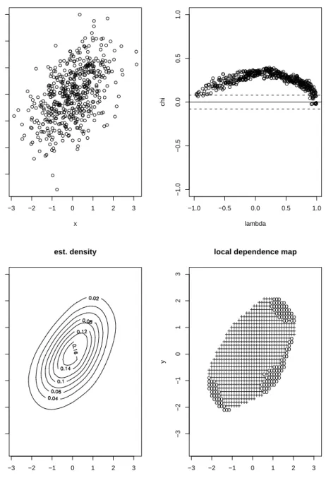
Y andX have a joint standard normal distribution with correlationρ= 0.5 is used. Nothing surprising can be recognized at the local dependence map. Positive dependence is indicated over almost the complete range looked at. The chi-plot shows a bent course. The chi-values are near to zero on the edges of the graph. For easier interpretation the mapping is extended by two
horizontal lines at±c/n1/2, where c is selected so that approximately 95%
of the pairs (λi, χi) lie between the lines. c can be calculated with Monte
Carlo methods (Fisher and Switzer, 2001).
The bent course of the chi-plots reports the so-called “tail independence“
characteristic of the bivariate normal distribution, provided that |ρ| < 1.
Tail dependence is often defined in terms of the copula of a joint distribu-tion. For a complete treatment of copula see Joe (1997). For a bivariate
distribution F(x, y) with j-th univariate margin Fj, the copula associated
withF is a distribution function C: [0,1]2→[0,1] that satisfies
F(x, y) =C(F1(x), F2(y)), x, y∈R. (13)
So the copula is a distribution function of a random vector,U = (U1, U2),
where eachUj ∼unif orm(0,1). If a bivariate copulaC is such that
lim
u→0C(u, u)/u=λL (14)
exists, C has lower tail dependence if λL ∈ (0,1] and no lower tail
depen-dence if λL = 0. Similarly the upper tail dependence can be defined (see
Joe, 1997).
The chi-value is zero if P(X ≤ u1, Y ≤u2) =P(X ≤u1)·P(Y ≤u2).
This is equal to C(u1, u2) =u1·u2 (15) and C(u1, u2) u1 =u2 resp. C(u1, u2) u2 =u1. (16)
If the copula is lower tail independent, we know that limu→0C(u, u)/u= 0
and so the chi-values are also equal to zero. For the normal distribution it is known that it is not tail dependent (Embrechts et al., 2002) and the chi-plot shows exactly this.
The bivariate t-distribution provides an interesting contrast to the
bi-variate normal distribution, provided ρ > −1 the copula of the bivariate
−3 −2 −1 0 1 2 3 −3 −2 −1 0 1 2 3 scatterplot x y −1.0 −0.5 0.0 0.5 1.0 −1.0 −0.5 0.0 0.5 1.0 chiplot lambda chi x y −3 −2 −1 0 1 2 3 −3 −2 −1 0 1 2 3 est. density −3 −2 −1 0 1 2 3 −3 −2 −1 0 1 2 3
local dependence map
x y + + + + + + + + + + + + + + + + + + + + + + + + + + + + + + + + + + + + + + + + + + + + + + + + + + + + + + + + + + + + + + + + + + + + + + + + + + + + + + + + + + + + + + + + + + + + + + + + + + + + + + + + + + + + + + + + + + + + + + + + + + + + + + + + + + + + + + + + + + + + + + + + + + + + + + + + + + + + + + + + + + + + + + + + + + + + + + + + + + + + + + + + + + + + + + + + + + + + + + + + + + + + + + + + + + + + + + + + + + + + + + + + + + + + + + + + + + + + + + + + + + + + + + + + + + + + + + + + + + + + + + + + + + + + + + + + + + + + + + + + + + + + + + + + + + + + + + + + + + + + + + + + + + + + + + + + + + + + + + + + + + + + + + + + + + + + + + + + + + + + + + + + + + + + + + + + + + + + + + + + + + + + + + + + + + + + + + + + + + + + + + + + + + + + + + + + + + + + + + + + + + + + + + + + + + + + + + + + + + + + + + + + + + + + + + + + + + + + + + + + + + + + + + + + + + + + + + + + + + + + + + + + + + + + + + + + + + + + + + + + + + + + + + + + + + + + + + + + + + + + + + + + + + + + + + + + + + + + + + + + + + + + + + + + + + + + + + + + + + + + + + + + + + + + + + + + + + + + + + + + + + + + + + + + + + + + + + + + + + + + + + + + + + + + + + + + + + + + + + + + + + + o o o o o o o o o o o o o o o o o o o o o o o o o o o o o o o oo o o o o o o o o o o o o o o o o o o o o o o o o o o o o o o o o o o o o o o o o o o o o o o o o o o o o o o o o o o o o o o o o o o o o o o o o o o o o o o o o o o o o o o o o o o o o o o o
Figure 1: Scatterplot, chi-plot, density estimation and local dependence map for normal distributed data
−8 −6 −4 −2 0 2 4 −15 −10 −5 0 5 10 scatterplot x y −1.0 −0.5 0.0 0.5 1.0 −1.0 −0.5 0.0 0.5 1.0 chiplot lambda chi x y −8 −6 −4 −2 0 2 4 −15 −10 −5 0 5 10 est. density −4 −2 0 2 4 −4 −2 0 2 4
local dependence map
x y + + + + + + + + + + + + + + + + + + + + + + + + + + + + + + + + + + + + + + + + + + + + + + + + + + + + + + + + + + + + + + + + + + + + + + + + + + + + + + + + + + + + + + + + + + + + + + + + + + + + + + + + + + + + + + + + + + + + + + + + + + + + + + + + + + + + + + + + + + + + + + + + + + + + + + + + + + + + + + + + + + + + + + + + + + + + + + + + + + + + + + + + + + + + + + + + + + + + + + + + + + + + + + + + + + + + + + + + + + + + + + + + + + + + + + + + + + + + + + + + + + + + + + + + + + + + + + + + + + + + + + + + + + + + + + + + + + + + + + + + + + + + + + + + + + + + + + + + + + + + + + + + + + + + + + + + + + + + + + + + + + + + + + + + + + + + + + + + + + + + + + + + + + + + + + + + + + + + + + + + + + + + + + + + + + + + + + + + + + + + + + + + + + + + + + + + + + + + + + + + + + + + + + + + + + + + + + + + + + + + + + + + + + + + + + + + + + + + + + + + + + + + + + + + + + + + + + + + + + + + + + + + + + + + + + + + + + + + + + + + + + + + + + + + + + + + + + + + + + + + + + + + + + + + + + + + + + + + + + + + + + + + + + + + + + + + + + + + + + + + + + + + + + + + + + + + + + + + + + + + + + + + + + + + + + + + + + + + + + + + + + + + + + + + + + + + + o o o o o o o o o o o o o o o o o o o o oo o o o o o o o o o o o o o o o o o o o o o o o o o o o o o o o o o o o o o o o o o o o o o o o o o o o o o o o o o o o o o o o o o o o o o o o −− −
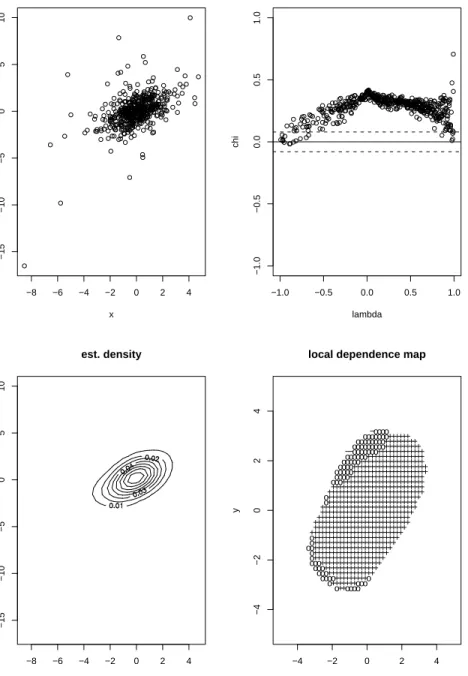
Figure 2: Scatterplot, chi-plot, density estimation and local dependence map for t-distributed data
−200 0 200 400 −7000 −6000 −5000 −4000 −3000 −2000 −1000 0 scatterplot x y −1.0 −0.5 0.0 0.5 1.0 −1.0 −0.5 0.0 0.5 1.0 chiplot lambda chi xtr ytr −4 −2 0 2 4 −4 −2 0 2 4 est. density −4 −2 0 2 4 −4 −2 0 2 4
local dependence map
x y + ++ + + + + + + + + + + + + + + + + + + + + + + + + + + + + + + + + + + + + + + + + + + + + + + + + + + + + + + + + + + + + + + + + + + + + + + + + + + + + + + + + + + + + + + + + + + + + + + + + + + + + + + + + + + + + + + + + + + + + + + + + + + + + + + + + + + + + + + + + + + + + + + + + + + + + + + + + + + + + + + + + + + + + + + + + + + + + + + + + + + + + + + + + + + + + + + + + + + + + + + + + + + + + + + + + + + + + + + + + + + + + + + + + + + + + + + + + + + + + + + + + + + + + + + + + + + + + + + + + + + + + + + + + + + + + + + + + + + + + + + + + + + + + + + + + + + + + + + + + + + + + + + + + + + + + + + + + + + + + + + + + + + + + + + + + + + + + + + + + + + + + + + + + + + + + + + + + + + + + + + o o o o o o o o o o o o o o o o o o o o o o o o o o o o o o o o o o o o o o o o o o o o o o o o o o o o o o o o o o o o o o o o o o o o o o o o o o o o o o o o o o o o o o o o o o o o o o o o o o o o o o o o o o o o o o o o o o o o o o o o o o o o o o o o o o o o o o o o o o o o o o o o o o o o o o o o o o o o o o o o o o o o o o o o o o o o o o o o o o o o o o o o o o o o o o o o o o o o o o o o o o o o o o o o o o o o o o o o o o o o o o o o o o o o o o o o o o o o o o o o o o o o o o o o o o o o o o o o o o o o o o o o o o o o o o o o o o o o o o o o o o o o o o o o o o o o o o o o o o o o o o o o o o o o o o o o o o o o o o o o o o o o o o o o o o o o o o o o o o o o o o o o o o o o o o o o o o o o o o o o o o o o o o o o o o o o o o o o o o o o o o o o o o o o o o o o o o o o o o o o o o o o o o o o o o o o o o o o o o o o o o o o o o o o o o o o o o o o o o o o o o o o o o o o o o o o o o o o o o o o o o o o o o o o o o o o o o o o o o o o o o o o o o o o o o o o o o o o o o o o o o o o o o o o o o o o o o o o o o o o o o o o o o o o o o o o o o o o o o o o o o o o o o o o o o o o o o o o o o o o o o o o o o o o o o o o o o o o o o o o o o o o o o o o o o o o o o o o o o o o o o o o o o o o o o o o o o o o o o o o o o o o o o o o o o o o o o o o o o o o o o o o o o o o o o o o o o o o o o o o o o o o o o o o o o o o o o o o o o o o o o o o o o o o o o o o o o o o o o o o o o o o o o o o o o o o o o o o o o o o o o o o o o o o o o o o o o o o o o o o o o o o o o o o o o o o o o o o o o o o o o o o o o o o o o o o o o o o o o o o o o o o o o o o o o o o o o o o o o o o o o o o o o o o o o o o o o o o o o o o o o o o o o o o o o o o o o o o o o o o o o o o o o o o o o o o o o o o o o o o o o o o o o o o o o o o o o o o o o o o o o o o o o o o o o o o o o o o o o o o o o o o o o o o o o o o o o o o o o o o o o o o o o o o o o o o o o o o o o o o o o o o o o o o o o o o o o o o o o o o o o o o o o o o o o o o o o o o o o o o o o o o o o o o o o o o o o o o o o o o o o o o o o o o o o o o o o o o o o o o o o o o o o o o o o o o o o o o o o o o o o o o o o o o o o o o o o o o o o o o o o o o o o o o o o o o o o o o o o o o o o o o o o o o o o o o o o o o o o o o o o o o o o o o o o o o o o o o o o o o o o o o o o o o o o o o o o o o o o o o o o o o o o o o o o o o o o o o o o o o o o o o o o o o o o o o o o o o o o o o o o o o o o o o o o o o o o o o o o o o o o o o o o o o o o o o o o o o o o o o o o o o o o o o o o o o o o o o o o o o o o o o o o o o o o o o o o o o o o o o o o o o o o o o o o o o o o o o o o o o o o o o o o o o o o o o o o o o o o o o o o o o o o o o o o o o o o o o o o o o o o o o o o o o o o o o o o o o o o o o o o o o o o o o o o o o o o o o o o o o o o o o o o o o o o o o o o o o o o o o o o o o o o o o o o o o o o o o o o o o o o o o o o o o o o o o o o o o o o o o o o o o o o o o o o o o o o o o o o o o o o o o o o o o o o o o o o o o o o o o o o o o o o o o o o o o o o o o o o o o o o o o o o o o o o o o o o o o o o o o o o o o o o o o o o o o o o o o o o o o o o o o o o o o o o o o o o o o o o o o o o o o o o o o o o o o o o o o o o o o o o o o o o o o o o o o o o o o o o o o o o o o o o o o o o o o o o o o o o o o o o o o o o o o o o o o o o o o o o o o o o o o o o o o o o o o o o o o o o o o o o o o o o o o o o o o o o o o o o o o o o o o o o o o o o o o o o o o o o o o o o o o o o o o o o o o o o o o o o o o o o o o o o o o o o o o o o o o o o o o o o o o o o o o o o o o o o o o o o o o o o o o o o − − − − − −−−−− − − − − − − − − − − − − − − − − − − − − − − − − − − − − − − − − − − − − − − − − − − − − − − − − − − − − − − − − − − − − − − − − − − − − − − − − − − − − − − − − − − − − − − − − − − − − − − − − − − − − − − − − − − − − − − − − − − − − − − − − − − − − − − − − − − − − − − − − − − − − − − − − − − − − − − − − − − − − − − − − − − − − − − − − − − − − − −− − − − − − − − − − − − − − − − − − − − − − − − − − − − − − − − − − − − − − − − − − − − − − − − − − − − − − − − − − − − − − − − − − − − − − − − − − − − − − − − − − − − − − − − − − − − − − − − − − − − − − − − − − − − − − − − − − − − − − − − − − − − − − − − − − − − − − − − − − − − − − − − − − − − − − − − − − − − −−
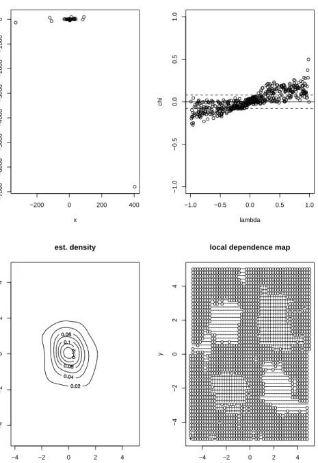
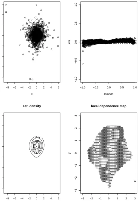
Figure 3: Scatterplot, chi-plot, density estimation and local dependence map for Cauchy distributed data
The data underlying the Figure 2 are from a t-distribution with three degrees of freedom. For the data generation the following qualities are used.
At first bivariate standard normal distributed samples Z with correlation
0.5 are produced. Aχ2 distributed variable U is then produced withdf = 3
degrees of freedom. WithV = (V1, V2)0 and Vi =√df Zi/√U, i= 1,2, the
variable V is then a sample from the t-distribution with three degrees of
freedom and
cov(V) = df
df−2Σ, (17)
Σ denoting the variance-covariance matrix of the bivariate normal variables. In comparison with the normal distributed data the chi-plot for the t-distributed data shows another course. The chi-plot does not incline on the right side of the graphic to the zero line anymore. This shows tail de-pendence on the upper right and lower left edge of the data. The local dependence map looks similar to the map for the normal distributed data. This changes in the next data example.
The data in Figure 3 are generated from a Cauchy distribution, in the same way as the t-distributed data. The degrees of freedom are set to one and the correlation of the bivariate standard normal is set to zero. The chi-plot in Figure 3 nevertheless shows dependence. Due to the definition of
λin (6), negative chi-values for negativeλmean negative dependence in the
upper left and lower right corner of the data. On the other hand, the positive
chi-values for positive λ indicate positive dependence in the lower left and
upper right corner. Looking at the local dependence map, one recognizes also four fields where dependencies are indicated. This confirms Holland
and Wang‘s (1987) observation thatγ(x, y) for the bivariate Cauchy density
“changes sign as(x, y)changes quadrant in the plane. Random variables X
andY are positively associated in the first and third quadrants and negatively associated in the second and fourth“. Exactly these signs are also shown in the local dependence map. This can be interpreted as positive association
between |X| and |Y|. The example shows, that the local dependence map
can be used to indicate dependence when the direction of the association is different in different regions of the plane.
4
Applications to stock return series
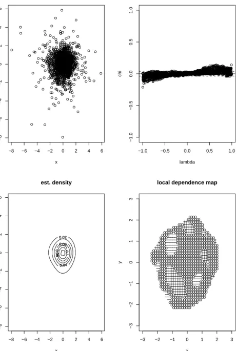
The local dependence graphs are used now to examine the “autocorrelation“ of two daily stock market index return series. The series are the German
DAX1 index from January 1, 1990 to Dezember 30, 1998 and the S&P 500
from January 1, 1992 until July 19, 1999. The returnsrt are defined by
rt= log pt
pt−1, (18)
with pt the price of the index at time t. The Figures 4 and 5 contain
scatterplots of rt against rt−1 for the respective return series. For both
indexes the chi-plots show dependencies. There are no dependencies in the center of the bivariate distributions but on the edges. So there seem to be tail dependencies in the lagged returns. Also in the local dependence maps spots with positive and negative dependence are recognized. The arrangement of the spots confirm the well known fact, that the lagged absolute returns are positively correlated. Both of the dependence graphs also show that the Bravais-Pearson correlation coefficient is not suitable to include the complex dependence structure in the lagged returns. The chi-plot shows in addition that when a model is developed for these data the tail dependence behavior has to be taken into account.
5
Summary
In the above sections two methods for local analysis of dependence were presented and illustrated at data examples. The first method, the chi-plot, is simple to calculate and is well suited to recognize dependence in the tails of the distribution. The second method, the local dependence map, is technically more demanding. It requires the estimation of mixed partial derivatives which is realized by nonparametric estimation methods. This also means that bandwidths must be chosen. After this the local depen-dence function must be converted with local permutation tests in the local dependence map. For this however regions can be indicated for the de-pendencies which are easy to interpret. Since regions with small densities are taken out of the calculations, the extreme tails of the distribution can not be analyzed. In summary, the two graphs are supplementary. The lo-cal dependence map delivers a mapping which is easy to interpret and the chi-plot permits representations of the dependencies up to the tails of the distribution.
−8 −6 −4 −2 0 2 4 6 −8 −6 −4 −2 0 2 4 6 scatterplot x y −1.0 −0.5 0.0 0.5 1.0 −1.0 −0.5 0.0 0.5 1.0 chiplot lambda chi x y −8 −6 −4 −2 0 2 4 6 −8 −6 −4 −2 0 2 4 6 est. density −3 −2 −1 0 1 2 3 −3 −2 −1 0 1 2 3
local dependence map
x y +++++ + + + + + + + + + + + + + + + + + + + + + + + + + + + + + + + + + + + + + + + + + + + + + + + + + + + + + + + + + + + + + + + + + + + + + + + + + + + + + + + + + + + + + + + + + + + + + + + + + + + + + + + + + + + + + + + + + + + + + + + + + + + + + + + + + + + + + ++ + + o o o o o o o o o o o o o o o o o o o o o o o o o o o o o o o o o o o o o o o o o o o o o o o o o o o o o o o o o o o o o o o o o o o o o o o o o o o o o o o o o o o o o o o o o o o o o o o o o o o o o o o o o o o o o o o o o o o o o o o o o o o o o o o o o o o o o o o o o o o o o o o o o o o o o o o o o o o o o o o o o o o o o o o o o o o o o o o o o o o o o o o o o o o o o o o o o o o o o o o o o o o o o o o o o o o o o o o o o o o o o o o o o o o o o o o o o o o o o o o o o o o o o o o o o o o o o o o o o o o o o o o o o o o o o o o o o o o o o o o o o o o o o o o o o o o o o o o o o o o o o o o o o o o o o o o o o o o o o o o o o o o o o o o o o o o o o o o o o o o o o o o o o o o o o o o o o o o o o o o o o o o o o o o o o o o o o o o o o o o o o o o o o o o o o o o o o o o o o o o o o o o o o o o o o o o o o o o o o o o o o o o o o o o o o o o o o o o o o o o o o o o o o o o o o o o o o o o o o o o o o o o o o o o o o o o o o o o o o o o o o o o o o o o o o o o o o o o o o o o o o o o o o o o o o o o o o o o o o o o o o o o o o o o o o o o o o o o o o o o o o o o o o o o o o o o o o o o o o o o o o o o o o o o o o o o o o o o o o o o o o o o o o o o o o o o o o o o o o o o o o o o o o o o o o o o o o o o o o o o o o o o o o o o o o o o o o o o o o o o o o o o o o o o o o o o o o o o o o o o o o o o o o o o o o o o o o o o o o o o o o o o o o o o o o o o o o o o o o o o o o o o o o o o o − − − − − − − − − − − − − − − − − − − − − − − − − − − − − − − − − − − − − − − − − − − − − − − − − − − − − − − − − − − − − − − − − − − − − − − − − − − − − − − − − − −− −
Figure 4: Scatterplot, chi-plot, density estimation and local dependence map for lagged daily DAX returns
−8 −6 −4 −2 0 2 4 6 −8 −6 −4 −2 0 2 4 6 scatterplot x y −1.0 −0.5 0.0 0.5 1.0 −1.0 −0.5 0.0 0.5 1.0 chiplot lambda chi x y −8 −6 −4 −2 0 2 4 6 −8 −6 −4 −2 0 2 4 6 est. density −3 −2 −1 0 1 2 3 −3 −2 −1 0 1 2 3
local dependence map
x y + + + + + + + + + + + + + + + + + + + + + + + + + + + + + + + + + + + + + + + + + + + + + + + + + + + + + + + + + + + + + + + + + + + + + + + + + + + + + + + + + + + + + + + + + + + + + + + + + + + + + + + + + + + + + + + + + + + + + + + + + + + + + + + + + + + + + + + + + + + o o o o o o o o o o o o o o o o o o o o o o o o o o o o o o o o o o o o o o o o o o o o o o o o o o o o o o o o o o o o o o o o o o o o o o o o o o o o o o o o o o o o o o o o o o o o o o o o o o o o o o o o o o o o o o o o o o o o o o o o o o o o o o o o o o o o o o o o o o o o o o o o o o o o o o o o o o o o o o o o o o o o o o o o o o o o o o o o o o o o o o o o o o o o o o o o o o o o o o o o o o o o o o o o o o o o o o o o o o o o o o o o o o o o o o o o o o o o o o o o o o o o o o o o o o o o o o o o o o o o o o o o o o o o o o o o o o o o o o o o o o o o o o o o o o o o o o o o o o o o o o o o o o o o o o o o o o o o o o o o o o o o o o o o o o o o o o o o o o o o o o o o o o o o o o o o o o o o o o o o o o o o o o o o o o o o o o o o o o o o o o o o o o o o o o o o o o o o o o o o o o o o o o o o o o o o o o o o o o o o o o o o o o o o o o o o o o o o o o o o o o o o o o o o o o o o o o o o o o o o o o o o o o o o o o o o o o o o o o o o o o o o o o o o o o o o o o o o o o o o o o o o o o o o o o o o o o o o o o o o o o o o o o o o o o o o o o o o o o o o o o o o o o o o o o o o o o o o o o o o o o o o o o o o o o o o o o o o o o o o o o o o o o o o o o o o o o o o o o o o o o o o o o o o o o o o o o o o o o o o o o o o o o o o o o o o o o o o o o o o o o o o o o o o o o o o o o o o o o o o o o o o o o o o o o o o o o o o o o o o o o o o o o o o o o o o o o o o o o o o o o o o o o o o o o o o o o o o o o o o o o o o o o o o o o o o o o o o o o o o o o o o o o o o o o o o o o o o o o o o o o o o o o o o o o o o o o o o o o o o o o o o o o o o o o o o o o o o o o o o o o o o o o o o o o o o o o o o − − − − −− − − − − − − − − − − − − − − − − − − − − − − − −− − − − − − −
Figure 5: Scatterplot, chi-plot, density estimation and local dependence map for lagged daily S&P 500 returns
6
Literature
Embrechts P., McNeil A., Strautmann D. (2002): Correlation and dependence in risk management: properties and pitfalls. In: Risk Man-agement: Value at Risk and Beyond, ed.: M.A.H. Dempster, Cambridge University Press, Cambridge.
Fisher N.I., Switzer P. (2001): Graphical assessment of dependence: is a picture worth 100 tests? The American Statistician, 55, 233-239.
Fisher N.I., Switzer P. (1985): Chi-plots for assessing dependence. Biometrika, 72, 253-265.
Hollander P.W., Wang Y.J. (1987): Dependence function for bivari-ate continuous densities. Communications in Statistics, Theory and Meth-ods, 16, 863-876.
Joe H. (1997): Multivariate models and dependence concepts. Chap-man and Hall, New York.
Jones M.C. (1998): Constant local dependence. Journal of Multivari-ate Analysis, 64, 148-155.
Jones M.C. (1996): The local dependence function. Biometrika, 83, 899-904.
Jones M.C., Koch I. (2002): Dependence maps: local dependence in practice. Discussion paper.
Loader C. (1999): Local regression and likelihood. Springer Verlag, Heidelberg.