Estudos e Documentos de Trabalho
Working Papers
5 | 2009
THE INTEREST RATE PASS-THROUGH OF THE PORTUGUESE BANKING SYSTEM: CHARACTERIZATION AND DETERMINANTS
Paula Antão
April 2009
The analyses, opinions and findings of these papers represent the views of the authors, they are not necessarily those of the Banco de Portugal or the Eurosystem.
Please address correspondence to Paula Antão
Economics and Research Department
Banco de Portugal, Av. Almirante Reis no. 71, 1150-012 Lisboa, Portugal; Tel.: 351 21 313 0418, Email: [email protected]
BANCO DE PORTUGAL
Edition
Economics and Research Department Av. Almirante Reis, 71-6th
1150-012 Lisboa www.bportugal.pt
Pre-press and Distribution Administrative Services Department
Documentation, Editing and Museum Division Editing and Publishing Unit
Av. Almirante Reis, 71-2nd
1150-012 Lisboa
Printing
Administrative Services Department Logistics Division Lisbon, April 2009 Number of copies 170 ISBN 978-989-8061-72-0 ISSN 0870-0117 Legal Deposit No 3664/83
The interest rate pass-through of the Portuguese banking
system: characterization and determinants
Paula Antão
April 2, 2009
Abstract
Using micro level data, this work characterizes the interest rate pass-through in loan and deposit retail rates of the Portuguese banking system. It concludes that the long-run impact of a change in money market rates on loans is typically around one while it is smaller than one for deposits. Moreover, di¤erences between the long run coe¢ cients for the corporate and household sectors also emerge. Results on the speed of adjustment show that, in general, deposit interest rates adjust faster than loan interest rates. The determinants of the heterogeneous behavior of banks in terms of interest rates’decisions are also studied. Capital and liquidity characteristics of banks turn out to be non-signi…cant while market share proves to contribute to a slower speed of adjustment in both loan and deposit interest rates.
JEL codes: G21, E43
.
I gratefully acknowledge António Antunes, Nuno Gonçalo Ribeiro and Paulo Rodrigues for their most relevant comments. I also acknowledge Carlos Robalo Marques for his help in early stages of the work.
1
Introduction
The speed of price adjustments to changes in market conditions is one of the factors underlying economic e¢ ciency. Retail interest rates on bank products are an example of such a relevant price. Everyday households and …rms are faced with these prices when making investment and savings decisions. In the euro area this is even more important because corporate …nancing is predom-inantly bank-based, in contrast to the United States, where market …nancing is more relevant. Additionally, euro area households hold most of their wealth under the form of deposits, although there has been a change in preferences towards other instruments, such as investment funds (see ECB, 2002). In this context, this study aims at understanding the interest rate pass-through of Portuguese banks, that is, how retail interest rates relate to changes in market conditions. This study has two main objectives. First, it characterizes the interest rate pass-through in retail rates of the Portuguese banking system. Second, it studies the determinants of the heterogeneous behavior of banks in terms of interest rate decisions.
The pass-through of market interest rates to retail interest rates has been studied for many years. In particular, the advent of the Economic and Monetary Union contributed to the substan-tial increase of articles discussing this topic in the euro area, inter alia focusing on cross section di¤erences among countries and accessing the degreee of integration1. Most studies analyse the
pass-through both in terms of the degree of the pass-through and of the speed of adjustment. In the majority of cases, studies consider aggregate interest rate series for di¤erent countries (and the euro area) on di¤erent interest rate categories2 and study whether there is pass-through
het-erogeneity across euro area countries and across di¤erent bank products. More recently, some micro-data studies on individual countries have also been performed3. Studies di¤er because data
used have di¤erent sources4 and also because they may refer to di¤erent time periods5. There
are also di¤erences in terms of the market interest rates considered: some studies select market rates with short maturity while others choose a market interest rate with a maturity more in line
1For a survey of recent studies on this topic see Sorensen and Werner (2006).
2See, for instance, De Bondt, Mojon and Valla (2005), Sorensen and Werner (2006) and Leuvensteijn, Sorensen,
Bikker, and van Rixtel (2008) with results for individual countries and the whole euro area.
3See, among others, Weth (2002) on German banks, De Graeve, de Jonghe and Vennet (2004) for Belgium,
Gambacorta (2004) for Italy, Lago-González and Salas-Fumás (2005) for Spain and Fuertes and He¤ernan (2006) for the United Kingdom.
4Most studies use national retail interest rate statistics collected by central banks. For euro area contries MFI
interest rates (MIR) statistics collected by the Eurosystem of Central Banks are also used, both for studies on individual countries and the euro area as a whole. Other data sources are also used; for instance, Leuvensteijn et al. (2008) use data from Bankscope.
with the repricing period of the bank product. In terms of econometric methods, most studies use single equation error correction models, which have the advantage of combining a long-run equilibrium relationship and short term adjustment dynamics to the long-run equilibrium.
Although studies approach the topic very di¤erently, two main conclusions emerge for European countries and the euro area. The …rst one is that there is signi…cant heterogeneity in the degree and speed of pass-through accross euro area countries. Some tentative explanations for this interest rate heterogeneous behavior are national di¤erences in bank competition, bank cost structures, banking ownership and legal and regulatory systems6. The second conclusion is that the heteregoneity in
the pass-through, both in terms of degree and speed, is also substantial across bank products. Most studies suggest that rates on loans to enterprises, specially short-term loans, adjust faster and show a more complete pass-through than interest rates on loans to households or on saving deposits. Results on deposits are not as clear as results on loans. Any way, the evidence shows
that interest rates on deposits are stickier than on loans. However, across studies, results are not uniform, which could happen because studies cover di¤erent time periods or because they use di¤erent market rates.
Against this background, this study develops an analysis of the interest rate pass-through of Portuguese banks. Some of the already mentioned studies present results for Portugal. These studies use aggregate data. Here, micro level data covering the period from January 1990 to December 2002 is used to study the interest rate pass through on a total of …fteen bank products (nine loan and six deposit interest rate categories). Despite the di¤erence in data sources, type of data and time period covered, results on the size of interest rate pass-through are broadly in line with the results from previous studies7. We conclude that there is a clear di¤erence in the long-run impact of a change in money market rates on loans and deposits. In the case of loans, the e¤ect is typically around one, meaning that changes in money market rates are fully transmitted to retail rates. In contrast, the long term coe¢ cient for deposits is smaller than one in all products considered. Under certain assumptions, this parameter can be also interpreted as a measure of competition in the industry. In this sense, the market for the corporate sector seems to be more
6Sander and Kleimeier (2004), Sorensen and Werner (2006) and Leuvensteijn et al. (2008) discuss several reasons
to explain heterogeneity across euro area countries.
7See, among the most recent studies presenting individual results for Portugal Leuvensteijn et al. (2008),
Sorensen and Werner (2006), De Bondt, Mojon, and Valla (2005) and Sander and Kleimeier (2004). Results are also in line with the main conclusions in Banco de Portugal (1999). Older studies with individual results for Portugal are Cottarelli and Kourelis (1994), Donnay and Degryse (2001), Heinimann and Schuller (2002), Kleimeier and Sander (2002) and Sander and Kleimeier (2002). A brief summary of the main results of these studies for Portugal can be found in De Bondt, Mijon and Valla (2005).
competitive than the one for households. Results on the speed of adjustment show that, in general, deposit interest rates adjust faster than loan interest rates.
The second part of this study aims at explaining the heterogeneity found across Portuguese banks. One advantage of using micro-data is the possibility of studying the causes of the pass-through heterogeneity across banks. Several reasons have been pointed out to explain the hetero-geneity in interest rate pass-through accross banks. The most relevant ones are related to solvency, liquidity, diversi…cation of activities, costs, liability structure, market power, concentration of the market and credit risk8. In this study, we try to explain the behavior of banks operating in the
Portuguese market considering some of these reasons. Constraints of data do not allow a deep study on this topic, but some conclusions are obtained. The liquidity and solvency of banks do not prove to be relevant for the speed and size of the pass-through for both loan and deposit interest rates. The conclusion on the relevance of the capital ratio could be related to the restraints on
banking activities in the period precendent the one under analysis. In fact, in the 80’s, banking activities were constrained and banks were not always able to …nd pro…table investments, resulting in higher levels of capital. Then, the nineties were years of adjustment re‡ecting the deregulation of banking activities and, simultaneouly, the convergence of nominal interest rate convergence, which help to explain the increase in bank credit. Nevertheless, capital bu¤ers of Portuguese banks were relatively high during an important part of the period under analysis. The market share of banks seems to be relevant for the determination of the speed of adjustment for both loan and deposit interest rates. Results suggest that banks with higher market shares, which could be interpreted as a proxy for market power, adjust interest rates slower than banks with smaller market shares.
This article is organised as follows. The …rst part studies the interest rate pass through. It starts by presenting the data in Section 2.1 and the model underlying the analysis in Section 2.2. The results are presented in Section 2.3. The second part studies the determinants of the heterogeneity in the behavior of banks. It starts by presenting the characteristics of banks in Section 3.1 and Section 3.2 presents the empirical results. Finally, the main conclusions of this study are summarized in Section 4.
8See De Graeve, De Jonghe and Vennet (2004), Gambacorta (2004), Fuentes and He¤ernan (2005), and
2
Characterisation of the interest rate pass through
2.1
Data
In Portugal, as in most countries, aggregate bank retail rates are publicly availabe but bank-speci…c rates are not. Since 1990, the Bank of Portugal has been conducting a monthly inquiry asking banks the rates they o¤er on new contracts of credits and loans. The inquiry also collects data on the amounts of the new operations. In December 2002 the inquiry changed dramatically introducing di¢ culties in the construction of a long-term time series of data from 1990 on9. Hence, the main data set used in this study comprises monthly data on retail rates and the corresponding amounts of new loan and deposit products for the period from January 1990 to December 2002.
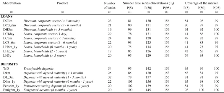
In this study we consider nine types of loan products (including discount operations) and six deposit products. These products were chosen as the most relevant in the period both for the corporate and the household sectors and for short and long maturities. Table 1 describes the data series and the abbreviations used to present the results. It also presents some cross-section and time-series characteristics of the series. The frequency of the entire analysis is monthly. The
information on interest rates for each product corresponds to a panel data where i denotes the
bank andTi denotes the number of months for which there is information for banki. The smallest panel is the one on "Discount, households with maturity less than 3 months (DH3m)", which considers only 16 banks, and the largest is the panel on "Transferable deposits (TrD)" including 34 banks. Panels for di¤erent products may cover di¤erent banks, as expected. Each panel data is unbalanced, that is, data from di¤erent banks(i)in the same panel cover di¤erent time periods (Ti). The study considers only the banks for which there is a time series of, at least, 72 consecutive monthly observations. For 50% of the banks considered, the time series have between 114 and 156 monthly observations as reported in column (5) of Table 1 (these values correspond to products "Loans, households with maturity between 6 months and 1 year (LH6m_1y)" and "Deposits with agreed maturity betwenn 6 months and 1 year (D6m_1y)", respectively). Table 1 also presents information on the coverage of the data, as the study does not consider all banks but just a sample of banks. Bank operations included in each panel account for around 80% of the new operations for each product, although there are some di¤erences in what concerns the coverage of the data. For instance, for 50% of the months considered, the 17 banks included in the panel
9At the end of 1997 the inquiry was slightly changed but it is possible to conciliate the outputs of both inquiries.
The same is not true from 2002 on as, since this date, retail interest rates has been collected following the rules of the European Central Bank set in December 2001 (Regulation no 63/2002).
Table 1: Characterization of data.
Abbreviation Product Coverage of the market P(5) P(50) P(95) P(5) P(50) P(95)
(1) (2) (3) (4) (5) (6) (7) (8) (9)
LOANS
DC3m Discount, corporate sector (< 3 months) 23 81 130 156 81 98 99 DC3_6m Discount, corporate sector (3 - 6 months) 21 80 131 156 80 97 99 DH3m Discount, households (< 3 months) 16 99 131 156 64 92 100 LC1day Loans, corporate sector (1 day) 29 78 131 156 41 88 100 LC3m Loans, corporate sector (< 3 months) 24 81 128 156 49 82 97 LC3_6m Loans, corporate sector (3 - 6 months) 22 93 125 156 41 83 99 LH6m_1y Loans, households (6 months - 1 year) 20 75 114 156 41 75 97 LH2_5y Loans, households (2 - 5 years) 17 85 126 156 42 65 97 LH5y Loans, households (> 5 years) 20 95 129 156 76 93 100
DEPOSITS
TrD Transferable deposits 34 95 142 156 95 99 100 D1m Deposits with agreed maturity (< 1 month) 25 85 120 153 58 81 97 D1_3m Deposits with agreed maturity (1 - 3 months) 32 78 137 156 81 91 99 D6m_1y Deposits with agreed maturity (6 months - 1 year) 22 103 156 156 95 98 100 Pens6m_1y Pensioneers'saving deposits (6 months -1 year) 20 102 139 156 81 97 99 Emig6m_1y Emigrants' account (6 months -1 year) 20 100 145 156 98 100 100
Number of banks
Number time series observations (Ti)
Notes: This table presents the abbreviation and a short description of each product in columns (1) and (2). Column (3) presents the number of banks included in the sample for each product. Columns (4) to (6) present the percentiles 5, 50 and 95 of the number of consecutive observations (out of 156 months) for each product. Columns (7) to (9) present percentiles 5, 50 and 95 of the value of new operations originated by the banks in the sample as a percentage of total value of new operations, for each product. All data is monthly.
"Loans, households (2 - 5 years)" account for only 65 percent of the total amount of new loans granted to households with a maturity between 2 and 5 years. In general, the coverage of the new operations of deposit products is higher than the one for loan products.
To perform this study we also use the money market interest rates of di¤erent maturities, which are publicly available. The money market interest rate series was constructed considering the information on unsecured transactions made in the domestic Interbank Money Market for the period between January 1990 and November 1992. These transactions are processed and settled through SITEME - Markets Electronic Transfer System. It then considers information on Lisbor (Lisbon Interbank O¤ered Rate) for the period December 1992 - December 1998 and Euribor rates from January 1999 onwards. We considered two di¤erent money market interest rate series, one with 3-month maturity and another with a 6-month maturity. It would have been interesting to consider a money market interest rate with a longer maturity, such as one year but it was not possible to construct such time series due to the lack of information for some months considered in the study. Besides, the transaction volumes at this maturity are much smaller and less representative of interbank dealings. Further, long term interest rates such as 5 or 10 year government bond yields are not used in this study because an overwhelming majority of the operations are either short-term or carry ‡oating interest rate.
Some authors argue that the best way do deal with this type of events is to consider merged banks as just one institution in the whole sample period. This approach is not followed here. We consider banks involved in a merger as di¤erent institutions before the merger. In this way, we are allowing interest rate policies to be di¤erent before and after the merge. The disadvantage of this approach is that we will have an unbalanced panel of data as, after the merge, the merged instituition is absorbed by the acquirer and will not make interest rate decisions.
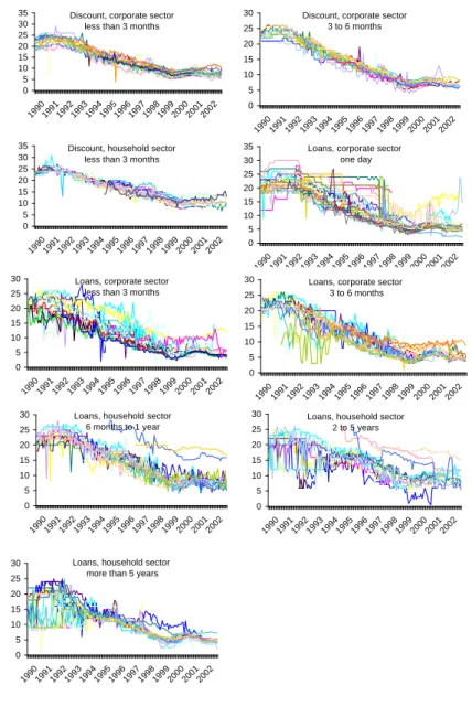
Appendix 1 presents a set of graphs depicting the retail rate series used in the study and also the money market interest rates. Data shows that interest rates have been decreasing over most of the sample period. This behavior results from the nominal convergence of the Portuguese economy in the process that led to the participation in the third stage of the Economic and Monetary Union in 1 January 1999. In general, bank retail rates tend to follow the evolution of money market interest rates except in the case of transferable deposits. There are also some di¤erences in the
retail rates charged by di¤erent banks within a panel, which suggest the study of bank speci…c characteristics in setting interest rates.
2.2
The model
The model follows closely the work by Hannan 1991 (see Appendix 2 for more details). The long run equations to be estimated are:
8 < : rin L =ain+binrs+"in rDim=aim+bimrs+"im where rin
L (rdim) represent the interest rate associated with the nth (mth) category of loans (de-posits) held by bank iandrs is the interbank market interest rate (either a 3-month or a 6-month interest rate). Given the asumptions of this model, parameter bin (bim) is a function of the elas-ticity of demand for bank i’s nth (mth) category of loans (deposits), and ain (aim) is a function of both the elasticity of demand for banki’s products and the corresponding marginal cost.
Under the hypotheses of the model, parameters b can be used as a measure of competition in
each banking product since values close to one correspond to a more competitive market. This parameter measures also the rate of a bank transmission of changes in the money market rate to their own retail rate.
The model presented must be carefully applied to interest rate time series since these series tend to be non-stationay. In that case, this model presents a long-run equilibrium relationship between
retail rates and the money market interest rate. In such case, the study of the relationship between non-stationary, but cointegraded variables, should be done by estimating an error correction model (ECM) as these models allow for a decomposition between the long-run equilibrium relationship and the short-run adjustments towards the long-run equilibrium. In this sense, this study starts by studying the stationarity of the retail rates and the money market interest rate and their cointegration relationships. If non-stationarity of the retail rates and the money market rates and cointegration between these variables is not rejected, an error correction model is estimated in order to capture both long term and short term e¤ects.
The estimation of an error correction representation will be done in two steps. The …rst step consists in estimating the cointegration vector
ri;t =ai+birs;t+ui;t: (1)
The intercept parameterais a measure of mark-up, or mark-down, that is, it measures how much
a retail rate is marked above or below the money market interest rate. The parameter b captures the long run pass-through, that is, it measures the fraction, or multiple, of the money market interest rate changes that is re‡ected in the bank retail interest rate.
In the second step we use the estimated residual of the cointegration vector to estimate an error correction model:
ri;t = i+ p X k=1 ik ri;t k+ q X l=0 il rs;t l+ iui;t 1+"i;t (2)
where ui;t 1 are the lagged residuals from individual cointegrating regressions. The residuals "i;t are assumed to be iid(0; 2): The term
iui;t 1 captures the adjustment towards equilibrium and
a signi…cant negative i is consistent with the series being cointegrated. The error correction
parameter i is the speed of adjustment and shows how much of the gap created by a change in
the money market interest rate is closed in one month.
2.3
Results
2.3.1 Stationarity and Cointegration Tests
We start by performing some panel unit root tests to check the stationarity of all series. It is well known that standard Dickey-Fuller-type tests lack power in small samples in distinguishing the unit root null from stationary alternatives. Adding the cross-section dimension to the time-series dimension allows for the use of unit root tests with more power.
Testing for unit roots in panel data has become more common given the development of testing procedures and their incorporation into econometric software packages10. However, most packages
work with balanced panel data while the data used in this study is unbalanced. We used the Rats procedure developed by Peter Pedroni which computes unit root tests based on the work by Levin, Lin and Chu (2003) and Im, Pesaran and Shin (2003). All these tests take as the null hypothesis non-stationarity and test against the alternative of stationarity11.
Let fyitg be the data series for a panel of banks, i= 1; :::; n; and let each bank series contain
t = 1; :::; Ti time series observations. The number of time series observations is di¤erent between banks and varies between 73 and 156 months. The number of banks in each panel ranges from 16 to a maximum of 34 (see Table 1). We wish to determine whether fyitg is integrated for each individual in the panel. As in the case of a single time series, the individual regression may include an intercept only or an intercept and time trend. The basic unit root testing approach by Levin,
Lin and Chu (2003), hereafter LLC, assumes that fyitg is generated by one of the following three models: Model 1 yit = yi;t 1+ pi X L=1 iL yi;t L+eit (3) Model 2 yit = i+ yi;t 1+ pi X L=1 iL yi;t L+eit (4) Model 3 yit= i+ it+ yi;t 1+ pi X L=1 iL yi;t L+eit; (5)
whereyit is the dependent variable of the model with dimension n X
i=1
Ti x 1, andeit areIID(0; 2e)
residuals. In Model 1, the panel unit root test procedure evaluates the null hypothesisH0 : = 0 against the alternative H1 : <0: In Model 2, the series yit has an individual speci…c mean but does not contain a time trend. In this case, the test evaluates the null hypothesis thatH0 : = 0 and i = 0;for all i; againstH1 : <0and i 2R: Finally, under Model 3, the series yit has an individual speci…c mean and time trend. The test procedure evaluates the null hypothesis that
H0 : = 0 and i = 0; for all i; against H1 : <0and i 2R:
In this study, yit is a series of monthly retail rates o¤ered by banks in both new operations of loans and deposits during the period between 1990 and 2002. On the one hand, it is reasonable
10See Harris and Sollos (2003) for a discussion on stationarity and cointegration tests with panel data.
11Many other nonstationarity tests heave been developed, such as the ones by Harris and Tzavalis (1999),
Breitung (2000) and Maddala and Wu (1999). All these tests take as the null hypothesis the presence of a unit root, and test against alternatives involving stationarity. In contrast, Hadri (2000) proposed a test for the null of stationarity against the alternative of unit roots in the panel data.
to admit that i 6= 0; as each bank has its own speci…cities. On the other hand, although during the sample period the interest rates showed clearly to be decreasing, this behavior is not expected to persist asymptotically. Such behavior would impose nominal rates to fall below zero. Consequently, we did not consider the presence of a time trend when explaining the behavior of interest rates. To sum up, the best model to analyse fyitg seems to be Model 2 and this is the one used to test the nonstationarity of all series.
A major assumption of all LLC tests is the imposition of homogeneity by setting i = ; for
all i. Thus, under the null all series in the panel contain a unit root, while the alternative is that all individual series are stationary. The alternative hypothesis is clearly restrictive since it tests if all icross sections are stationary. Im, Pesaran and Shin (2003), hereafter IPS, relaxed the
homogeneity constraint by estimating the equations of Models 1 to 3 allowing i to vary freely
across the i individual series in the panel. The null hypothesis (H0 : i = 0) is that each series in the panel contains a unit root and the alternative hypothesis (H0 : i <0; for at least one i) is that at least one of the individual series in the panel is stationary12. Essentialy, the IPS test averages the ADF-individual unit root test statistics that are obtained from estimating equations such as (3), (4) or (5), for each i. A rejection of the null hypothesis indicates stationarity of the series.
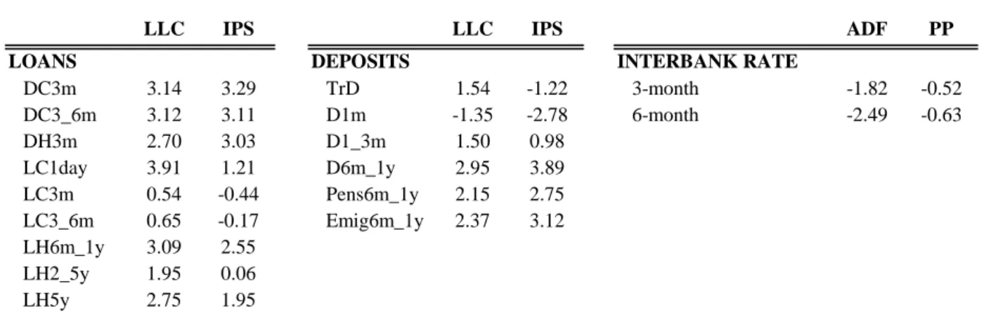
Table 2 presents the results of the LLC and IPS tests13 developed for all panels assuming Model 2. As both LLC and IPS test statistics follow a standard normal distribution N(0;1); we do not reject the null hypothesis of a unit root in bank interest rate series, at a nominal signi…cant level of 5%, if the statistics are larger than -1.645. For the money market interest rate we computed the Augmented Dickey and Fuller test as in Said and Dickey (1984) and the Phillips Perron (1988) assuming, once again, the model of equation (4). The test statistics are shown in Table 2 and
12Another problem of the LLC tests is related with the power of the tests to reject the null when it is false.
Harris and Tzavalis (1999) conducted Monte Carlo experiments to look at the properties of these tests when T is small. They analysed the power of the test to reject the null hipothesis when it is false. They found that the T ! 1assumption underlying LLC tests yields a test with poorer power properties, especially in …nite samples with T less than 50. They suggested testing for panel unit roots based on the assumption that T is …xed. As it was not possible to implement this test with unbalanced data, we tried to surpass this problem by choosing time series with as many observations as possible.
13To decide about the number of lags to include in all tests, we estimated the model y
it= i+
p X
L=1
iL yi;t L+
eit, for each i;choosing a maximum number of lags p= 12because data is monthly. Then we used the t-statistic
onbiL to determine if a smaller lag order is preferred. We observed thatL=p= 12 was a signi…cative lag for at
least one series of each panel, although for most series the highest signi…cative lag was smaller. As the software we used did not allow us to choose a di¤erent number of lags for each series within the panel, we decided to consider p= 12in all panels.
Table 2: Panel unit root test statistics
LLC IPS LLC IPS ADF PP
LOANS DEPOSITS INTERBANK RATE
DC3m 3.14 3.29 TrD 1.54 -1.22 3-month -1.82 -0.52 DC3_6m 3.12 3.11 D1m -1.35 -2.78 6-month -2.49 -0.63 DH3m 2.70 3.03 D1_3m 1.50 0.98 LC1day 3.91 1.21 D6m_1y 2.95 3.89 LC3m 0.54 -0.44 Pens6m_1y 2.15 2.75 LC3_6m 0.65 -0.17 Emig6m_1y 2.37 3.12 LH6m_1y 3.09 2.55 LH2_5y 1.95 0.06 LH5y 2.75 1.95
Notes: LLC stands for Levin, Lin and Chu (2003) test; IPS stands for Im, Pesaran and Shin (2003) test; ADF stands for Augmented Dickey and Fuller test proposed by Said and Dickey (1984) and PP stands for Phillips and Perron (1988) test. The lag length is set at 12 for all series. LLC and IPS test statistics are normally distributed and the 5% level critical value is -1.645. The ADF 5% and the PP 5% level critical value -2.887. The null of a unit root is not rejected at a 5% confidence level for all variables except the IPS test for Deposits with agreed maturity less than one month (D1m). The results were obtained using RATS. A short definition of each bank product can be found in Table 1.
allow us to not reject the null of a unit root in all interest rate series in the sample14.
As with testing for unit roots using panel data, testing for cointegration by pooling information across theimembers of the panel allows for power improvements. We used the cointegration tests developed by Pedroni (1999, 2004), where the null hypothesis is that there is no cointegration. Pedroni (1999, 2004) starts by computing regression residuals from the cointegration regression which, in the most general case may take the form
yit = i+ it+ J X j=1 jixji;t+eit (6) for t = 1; :::T; i= 1; :::N; j = 1; :::J
where T refers to the number of observations over time, N refers to the number of individual
members in the panel, andJ refers to the number of regression variables. As there are N di¤erent members in each panel, we can think ofN di¤erent equations each withM regressors. The various
slope coe¢ cients ji are allowed to vary across the i members of the panel. The parameter i is
the member speci…c intercept, or …xed-e¤ects parameter, and is also permited to vary across thei
member of each panel. This general form also allows to include deterministic time trends speci…c to individual members of the panel, captured by the term it: It is also possible to include a set of common time dummies that are intended to capture disturbances which may be shared across
the di¤erent members of the panel. Since i and ji are permited to vary, this approach allows
14The number of lags to include in the ADF test was decided following the same method as for the other interest
for considerable short-and long-run heterogeneity.
Tests for the null of no cointegration are based on the residuals beit using b
eit = ibeit 1+ it: (7) Pedroni (1999) presents seven di¤erent test statistics. The …rst four tests are based on what is commonly referred to as the within-dimension, and the last three tests are based on what is referred to as the between-dimension. The consequence of this distinction arises in terms of the autoregressive coe¢ cient i: For the within-dimension statistics, also called panel statistics, the test for the null of no cointegration is implemented in equation (7) as a test of the null hypothesis
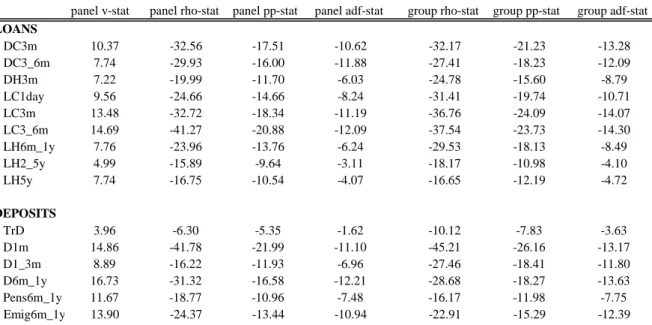
H0 : i = 1 for all i; versus the alternative H1 : i = < 0 for all i: These tests consider the existence of a common value for all i: The between-dimension test statistics, also called group mean statistics, by contrast, are implemented as tests of the null H0 : i = 1 for all i; versus the alternative H1 : i < 0 for all i: Thus, the between-dimension statistics allow to model an additional source of potential heterogeneity across individual members of the panel. The details of each test can be seen in Pedroni (1999). Under the alternative hypothesis, the …rst test proposed by Pedroni diverges to plus in…nity and thus the right tail of the standard normal distribuition needs to be used to reject the null hpothesis of no cointegration. For each of the other six tests, these diverge to minus in…nity and large negative values imply that the null of no cointegration is rejected. To implement Pedroni’s tests in unbalanced panels we used Rats15. The results are
presented in Table 3 and are based on a model without a time trend. Cointegration tests consider the 3-month interbank rate for products with a maturity less than 6 months and a 6-month interbank rate for products with a maturity higher than 6 months16. All tests reject the null of no
cointegration for all interest rate series. However, the test statistics for the variable "transferable deposits (TrD)" are not as high as for the other variables. The same tests were applied to a model with a time trend. In this case, the hypothesis that "transferable deposits (TrD)" is not cointegrated with the interbank rate is not rejected. This is consistent with Figure 2 of the retail rates of this product (see Appendix 1).
15The procedure used was "pancoint.src" downloaded from the RATS web-site written by Pedroni.
16In the case of deposits, the money market interest rate was corrected to consider minimum reserves
require-ments. Between January 1990 and October 1994 the reserve ratio was 17 percent and reserves were paid interest at a …xed rate decided by Banco de Portugal. During this period, the money market interest rate considered as the oportunity cost of deposit retail rate isrs(1 ) + r ;where is the reserve ratio andr measures the interest
rate paid on the amount of reserves. This remuneration rate is tipically lower than a market rate. In November 1994 the reserve ratio decreased to 2%, and reserves started to be paid a remuneration at a market rate.
Table 3: Panel cointegration test statistics
panel v-stat panel rho-stat panel pp-stat panel adf-stat group rho-stat group pp-stat group adf-stat
LOANS DC3m 10.37 -32.56 -17.51 -10.62 -32.17 -21.23 -13.28 DC3_6m 7.74 -29.93 -16.00 -11.88 -27.41 -18.23 -12.09 DH3m 7.22 -19.99 -11.70 -6.03 -24.78 -15.60 -8.79 LC1day 9.56 -24.66 -14.66 -8.24 -31.41 -19.74 -10.71 LC3m 13.48 -32.72 -18.34 -11.19 -36.76 -24.09 -14.07 LC3_6m 14.69 -41.27 -20.88 -12.09 -37.54 -23.73 -14.30 LH6m_1y 7.76 -23.96 -13.76 -6.24 -29.53 -18.13 -8.49 LH2_5y 4.99 -15.89 -9.64 -3.11 -18.17 -10.98 -4.10 LH5y 7.74 -16.75 -10.54 -4.07 -16.65 -12.19 -4.72 DEPOSITS TrD 3.96 -6.30 -5.35 -1.62 -10.12 -7.83 -3.63 D1m 14.86 -41.78 -21.99 -11.10 -45.21 -26.16 -13.17 D1_3m 8.89 -16.22 -11.93 -6.96 -27.46 -18.41 -11.80 D6m_1y 16.73 -31.32 -16.58 -12.21 -28.68 -18.27 -13.63 Pens6m_1y 11.67 -18.77 -10.96 -7.48 -16.17 -11.98 -7.75 Emig6m_1y 13.90 -24.37 -13.44 -10.94 -22.91 -15.29 -12.39
Note: These results were obtained for a model without a time trend. The interbank rate used for variables with a maturity smaller than 6 months is the 3-month interbank rate; for all the others it is the 6-month interbank rate. For deposit products the interbank rates were corrected to consider minimum reserve requirements. All reported values are distributed as N(0,1) under the null of no cointegration. The results were obtained using RATS. A short definition of each bank product can be found in Table 1.
2.3.2 Model estimation
The various panel cointegration estimators available include within- and between-group fully mod-i…ed (FMOLS) and dynamic (DOLS) estimators. So far there is no consensus on which estimator is prefered (see, for instance, Kao and Chiang, 2000 and Pedroni, 2000). However, the group mean
panel FMOLS estimator has the advantage of allowing for heterogeneity for all i in each panel.
This estimator is the one used in this study. Again, we used the Rats procedure17 developed
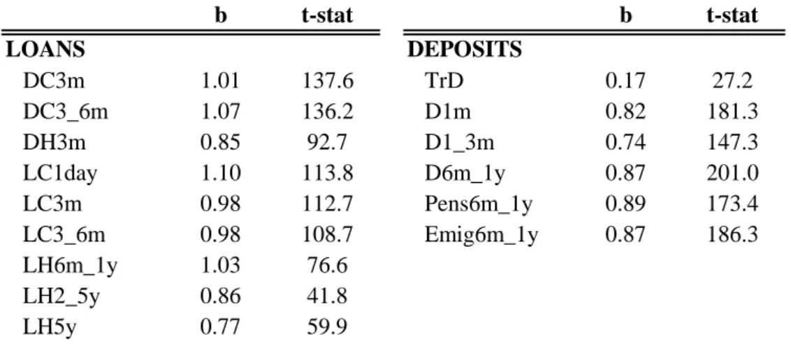
by Pedroni which computes a group mean panel FMOLS estimator based on equation (1). The results are presented in Table 4.
Bank retail rates are not expected to deviate from the money market interest rate for long periods and the cointegration tests con…rm that there is a long-run relationship between retail rates and the interbank rate. However, the impact of a unitary change in the interbank rate is di¤erent between loans and deposits. In the case of loans, the e¤ect is typically around one, meaning that changes in money market rates are fully transmitted to retail rates. On the other hand, the transmission of a change in interbank rates to deposits is shown to be incomplete. An usual explanation to the incomplete transmission of interbank rates to deposits retail rates is the presence of minimum reserve requirements. This di¤erence in the results for loans and deposits
Table 4: FMOLS estimator of the cointegrating Vector b t-stat b t-stat LOANS DEPOSITS DC3m 1.01 137.6 TrD 0.17 27.2 DC3_6m 1.07 136.2 D1m 0.82 181.3 DH3m 0.85 92.7 D1_3m 0.74 147.3 LC1day 1.10 113.8 D6m_1y 0.87 201.0 LC3m 0.98 112.7 Pens6m_1y 0.89 173.4 LC3_6m 0.98 108.7 Emig6m_1y 0.87 186.3 LH6m_1y 1.03 76.6 LH2_5y 0.86 41.8 LH5y 0.77 59.9
Note: The interbank rate used for variables with a maturity smaller than 6 months is the 3-month interbank rate; for all the others it is the 6-month interbank rate. For deposit products the interbank rates were corrected to consider minimum reserve requirements. The results were obtained using RATS. A short definition of each bank product can be found in Table 1.
was already observed in other studies on the Portuguese banking industry covering di¤erent time periods and using di¤erent methodologies (see Banco de Portugal, 1999, Sorensen and Werner, 2006, and De Bondt, Mijon and Valla, 2005). Moreover, the above mentioned studies for Portugal had di¤erent data sources and considered only aggregate data.
Although cointegration between the interest rates of "transferable deposits" and the interbank rate is not rejected in a model without trend, this conclusion does not hold for a model with a time trend. This was expected from the simple observation of Figure 2 with the evolution of retail rates in Appendix 1. This type of deposits may be seen as a way of starting a banking relationship, and a way to have access to other …nancial instruments. As such, they are more related with a payment service rather than an investment and their remuneration is quite low. As expected, retail rates of these deposits are not so responsive to the money market rate. Given the above discussion, the "transferable deposits" interest rates will not be analysed in this work.
Additionally, the existence of a risk premium in loan products was not yet taken into account.
If credit risk is incorporated in the model of Hannan (1991), it can be shown that parameter b
can be higher than one. This helps explaining the estimated values of b higher than one. In this context, we also computed a default measure and used it to estimate the long run parameter. This default measure is computed for each bank and does not depend on the speci…c produt considered. Using this default measure as another regressor in equation (1) the long run coe¢ cients of the interbank rate turn out to be equal or lower than the ones in Table 4, however this conclusion is
not valid for each bank individually.
The long run parameter can also be interpreted as a measure of competition in each particular market segment. If the market is competitive, this parameter should be around one. Under this interpretation, it can be argued that the credit market for corporations is more competitive than for households.
The next step consists in estimating the error correction model. As the long-run parameters are di¤erent between banks, equation (2) will be estimated individually for each bank. Thus, di¤erent estimates of the long-run parameters, instead of pooling the banks with respect to this parameter, will be used. We started by estimating the general expression in equation (2) with
p=q = 6and used the Schwarz Information Criterion to choose the number of lags to be included.
Keepingp= 6, the lagged terms of the di¤erence in the money market rate turned out to be non
signi…cant in most cases. We ended up with a model with p = 6 and q = 0: Results of the
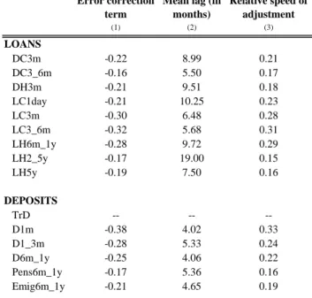
estimation are presented in Table 5. All columns present the arithmetic mean of the individual values obtained estimating each series individually. Results for the mean adjustment lag18 (mean lag) are also reported. Values for the "transferable deposits (TrD)" variable are not presented as already mentioned.
The error correction term, which can also be seen as a measure of the speed of adjustment of retail rates to changes in interbank rates is, in general, more negative for deposits than for loans19. It means that changes in the interbank rate result in faster changes in the retail rates of deposits than loans. This could be due to the fact that interest rates were declining over most of the sample considered. In addition, retail rates of loans to the corporate sector react faster to changes in the interbank rate. Another result is that there seems to exist a negative relationship between the maturity and the speed of adjustment for deposit rates (the error correction term for deposits with higher maturities presents lower values in absolute terms). Among loans, no clear relationship between the maturity and the speed of adjustment emerges.
The comparison of the speed of adjustment accross products needs to consider also the long-run equilibrium rates these retail rates are adjusting to. In other words, one should investigate whether retail rates are adjusting faster to a less than complete pass through, as in the case of deposits, or
18See Appendix 3 for a derivation of the mean lag in this model.
19This result contrasts with the results of Kok-Sorensen and Werner (2006) and Van Leuvensteijn et al. (2008).
In the …rst case, the speed of adjustment of consumer loans is higher than for mortgage loans, short term loans to enterprises and time deposits. In the second case, the speed of adjustment is approximately the same for mortgage loans, short term loans to enterprises and time deposits.
Table 5: Error correction term estimators and mean adjustment lag
Error correction term
Mean lag (in months) Relative speed of adjustment (1) (2) (3) LOANS DC3m -0.22 8.99 0.21 DC3_6m -0.16 5.50 0.17 DH3m -0.21 9.51 0.18 LC1day -0.21 10.25 0.23 LC3m -0.30 6.48 0.28 LC3_6m -0.32 5.68 0.31 LH6m_1y -0.28 9.72 0.29 LH2_5y -0.17 19.00 0.15 LH5y -0.19 7.50 0.16 DEPOSITS TrD -- -- --D1m -0.38 4.02 0.33 D1_3m -0.28 5.33 0.24 D6m_1y -0.25 4.06 0.22 Pens6m_1y -0.17 5.36 0.16 Emig6m_1y -0.21 4.65 0.19
Notes: Column (1) reports the arithmetic mean of the valuesγi obtained with the
individual estimation of equation (2). Column (2) reports the arithmetic mean of the individual mean lags. Finally, column (3) reports the arithmetic mean of the individual relative speed of adjustment computed as the product of -γiwith bi. A short definition
of each bank product can be found in Table 1.
slower to a higher value of pass-through, as in the case of loans. We then compute a measure of relative adjustment by multiplying the error correction term by the long term multiplier for each bank. The average of this measure, for each product, is presented in the last column of Table 5. Although the relative speed of adjustment measure is still higher for deposits, the di¤erence is now smaller when compared with the same measure for loans.
3
The determinants of the interest rate pass through
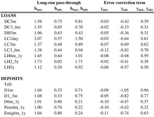
Most studies on pass-through analyze the impact of changes in money market interest rates on aggregate values, without taking into account the heterogeneity in the behavior of banks. However, the availability of bank individual data allows for the estimation of each relationship individually. Such detailed data allow us to study the price-setting behavior of banks, and their incentives to adapt their retail rates to changing market conditions. Using the individual estimations performed in the previous section, it is possible to conclude that there is some heterogeneity in the behavior of banks within a panel. Table 6 presents the minimum and maximum individual values obtained for the log-run coe¢ cient and the error correction term estimated in the previous section. It also reports a measure of the dispersion of the estimated values within each panel. As can be
Table 6: Heterogeneity of the long-run pass-through and the error correction term
bmax bmin bmax -bmin γmax γmin γmax -γmin
LOANS DC3m 1.56 0.75 0.81 -0.03 -0.42 0.39 DC3_6m 1.55 0.85 0.70 -0.02 -0.33 0.31 DH3m 1.06 0.63 0.43 -0.05 -0.36 0.31 LC1day 2.07 0.57 1.50 -0.03 -0.64 0.61 LC3m 1.37 0.48 0.89 -0.07 -0.69 0.62 LC3_6m 1.38 0.44 0.94 -0.12 -0.82 0.70 LH6m_1y 1.65 0.64 1.01 -0.08 -0.68 0.59 LH2_5y 1.73 0.02 1.71 -0.02 -0.41 0.39 LH5y 1.12 0.20 0.92 -0.06 -0.57 0.50 DEPOSITS TrD D1m 1.04 0.33 0.71 -0.09 -1.05 0.96 D1_3m 1.08 0.33 0.75 -0.05 -0.82 0.77 D6m_1y 1.01 0.80 0.21 -0.10 -0.47 0.37 Pens6m_1y 1.00 0.78 0.22 -0.10 -0.42 0.32 Emig6m_1y 1.04 0.80 0.24 -0.11 -0.74 0.63
Long-run pass-through Error correction term
Notes: bmax (bmin) is the maximum (minimum) long-run coefficient estimated using equation (1), within each panel. γmax (γmin) is the maximum (minimum) error correction term estimated using equation (2), within each panel. A short definition of each bank product can be found in Table 1.
observed, there is heterogeneity in the behavior of banks and this motivates the study of this section. Here we investigate whether bank characteristics explain the di¤erences obtained in the estimated coe¢ cients. The objective is to study the di¤erent decisions of banks in terms of their own speci…c characteristics. In addition, other characteristics such as the Her…ndahl index are also taken into account. In order to characterize the di¤erent behavior of banks, we regress the estimated value for the error correction term and the long term coe¢ cient on several bank and product characteristics. Loan products are considered as a group and deposits as another group implying that there is a common behaviour in the loan market and in the deposits market.
In the literature, several factors have been referred to as having an impact on the interest rate pass-through. According to the traditional structure-conduct-performance hypothesis, the setting of retail rates is less favorable to costumers in more concentrated markets as a result of competitive imperfections in these markets. Consequently, bank pro…ts are higher in more concentrated, or less competitive markets. A related theory is the relative market-power hypothesis. This theory asserts that only …rms with large market shares are able to exercise market power in pricing products and, consequently, earn higher pro…ts. These two market power hypothesis would predict a negative
impact on the pass-through, as banks in more concentrated markets, or with more market power, would be able to set interest rates more autonomously. In this study, as a measure of concentration,
we use the Her…ndahl index of each product and consider only new operations. Regarding the
computation of market shares, we opted to compute the market share of each bank in new
transactions of each product instead of a single market share taking into account the global activity of the bank.
In contrast to these market power theories, there are also e¢ ciency explanations of the positive relationship between pro…ts and either concentration or market shares. Banks may have higher pro…ts because they are more cost e¢ cient, either in terms of superior management, production technologies or because they work at more e¢ cient scales. These banks are also assumed to gain market share, resulting in more concentrated markets. However, in this case, the positive relationship between pro…ts and market power is spurious, as it is the e¢ ciency that is driving
both pro…ts and market structure. Following this hypothesis, e¢ cient banks have more incentive to pass its e¢ ciency advantage on to their customers, regardless of the evolution of market rates. A negative relationship between an e¢ ciency measure and the pass-through would be consistent with the e¢ ciency hypothesis. As it is not possible to construct the e¢ ciency measures proposed by Berger (1995), we decided to consider the cost to assets ratio as a measure of the degree of operational e¢ ciency.
In line with the literature on the credit channel of monetary policy transmission (for instance, Kishan and Opiela, 2000, and Kashyap and Stein, 2000), we included in the regressions an indicator of capitalization and an indicator of liquidity. Kishan and Opiela (2000) provide evidence that the loan supply of small, undercapitalized banks is more responsive to monetary policy than that of larger and well capitalized banks. As in the work by Kishan and Opiela (2000) we compute the
capital ratio as equity capital / total assets. On the other hand, Kashyap and Stein (2000)
study the monetary transmission mechanism using a data set of US commercial banks and …nd that the impact of monetary policy on lending is stronger for banks with less liquid assets. To test
this hypothesis, we use the coverage ratio of interbank liabilities by highly liquid assets
(interbank assets and assets eligible for monetary policy operations) as an indicatior of liquidity. Following this line of the literature, a negative relationship between the interest rate pass through and the capital and liquidity ratios would be expected.
deposits) provide more loan rate smoothing in response to exogenous credit shocks. The stable pool of deposits leave the banks less vulnerable to exogenous interest rate shocks. In line with
the work by Berlin and Mester (1999) we included a measure of a bank’s liability structure.
De Graeve, De Jonghe and Vennet (2004) argue that banks with more diversi…ed activites are less vulnerable to shocks in market interest rates than banks which are more specialized in retail activites. As such, more diversi…ed banks would set interest rates more autonomously than more specialized banks. The indicator used to measure the degree of diversi…cation is the ratio of non
interest income over gross income.
Another relevant variable in the determination of loan interest rates is the level of default risk of each bank’s portfolio. The ratio of non performing loans to toal loans is often used as a measure of default risk. However, this measure is quite sensitive to the evolution of credit and to write-o¤ policies. In the …rst case, the growth of credit in the up stages of the economic cycle contribute
to a (mechanic) decrease in non performing loans ratios, when usually it is in these stages of the cycle that credit risk builds up. In the second case, the write-o¤ of loans totally provisioned will make this ratio to decrease, specially in later stages of the cycle when loan delinquencies tend to increase. In this context, the variable used to measure credit risk is computed as the ratio of the
value of new non performing loans (over a year) to total loans. We expect a negative
relationship between default risk and the pass through of market rates as the setting of loan interest rates tends to follow less closely the evolution of market rates in situations where credit risk is more important.
Finally, other variables were introduced to consider some Portuguese banking characteristics. Throughout the 1980’s, the Portuguese banking system was subject to restrictions in several dimensions of its activities. These restrictions covered di¤erent features of the industry such as the setting of deposits and loans interest rates, the opening of new branches, the ownership of the institutions (many banks were public) and the entry of foreign banks. In the early nineties, the acceleration of the deregulation process promoted a dramatic change in the behavior of banking
institutions. Between 1993 and 2002, the number of branches20 increased around 70 per cent
and the number of banks increased around 50 per cent, from 43 banks (and branches of foreign banks) by the end of 1993 to 64 banks by the end of 2002. The privatisation process progressed and in 1997 the market share of state owned banks (in credits and deposits) was lower than 30 per cent. Simultaneously, a sequence of take-overs intensi…ed in the mid-eighties. Following
several acquisitions, banking business became more concentrated. The market share of the …ve major banking groups, in terms of assets21, went from 68 per cent in 1992 to 78 per cent in 2002,
reaching the highest value of 82 per cent in 2000. Another important fact is the increasing number of foreign bank entries in the Portuguese market. The number of foreign banks doubled in the nineties and the market share (either in assets or credits) more than doubled22. To sum up, during
the period under analysis the Portuguese banking business has been highly concentrated in …ve institutions, state-owned banks decreased in importance and foreign banks increased their weight in the industry. As a consequence, we decided to introduce several control variables, namelly a
dummy variable to control for the nationality of the bank, a dummy variable to control if the
bank belongs to one of the big …ve banking groups, and a growth variable measuring theasset
growthof the bank over time. The nationality issue is particularly relevant to take into account the fact that bank’s decisions in terms of price-setting may di¤er whether a bank belongs to a
foreign banking group as, in such case, these decisions are part of the group international decisions. The size issue is relevant as larger banks are expected to lend money to larger …rms which may have more …nancing sources than smaller …rms, which tend to be more dependent on bank loans. Thus, larger banks may follow market conditions more closely. In addition, to take into account the relevance of the new operations of the product being studied, an indicator of its weight to the broad category of credits or loans was also considered. Finally, the pro…tability of the bank
was also taken into account by introducing a pro…tability dimension measured by the ROE.
3.1
Data
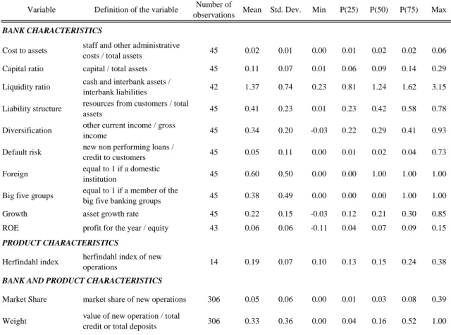
Bank characteristics are obtained by constructing ratios from balance sheets and pro…t and loss accounts of banks. The data used for the construction of all ratios matches the years studied in the previous sections. Outlier observations were considered missing and a correlation matrix was constructed to prevent the possibility of multicollinearity issues. Table 7 presents summary statistics of the data used in this section.
3.2
Results
The model to be estimated is the following
yi;j = + Xi+ Yj + Zi;j +"i;j (8)
21Market shares based on credit present a very similar evolution.
22However, the biggest jump in foreign banks’ market share occurred after the acquisition of a big portuguese
Table 7: Summary statistics on bank and product characteristics
Variable Definition of the variable Number of
observations Mean Std. Dev. Min P(25) P(50) P(75) Max
BANK CHARACTERISTICS
Cost to assets staff and other administrative
costs / total assets 45 0.02 0.01 0.00 0.01 0.02 0.02 0.06 Capital ratio capital / total assets 45 0.11 0.07 0.01 0.06 0.09 0.14 0.29 Liquidity ratio cash and interbank assets /
interbank liabilities 42 1.37 0.74 0.23 0.81 1.24 1.62 3.15 Liability structure resources from customers / total
assets 45 0.41 0.23 0.01 0.23 0.42 0.58 0.78 Diversification other current income / gross
income 45 0.34 0.20 -0.03 0.22 0.29 0.41 0.93 Default risk new non performing loans /
credit to customers 45 0.05 0.11 0.00 0.01 0.02 0.04 0.73 Foreign equal to 1 if a domestic
institution 45 0.60 0.50 0.00 0.00 1.00 1.00 1.00 Big five groups equal to 1 if a member of the
big five banking groups 45 0.38 0.49 0.00 0.00 0.00 1.00 1.00 Growth asset growth rate 45 0.22 0.15 -0.03 0.12 0.21 0.30 0.85 ROE profit for the year / equity 43 0.06 0.06 -0.11 0.04 0.07 0.09 0.15
PRODUCT CHARACTERISTICS
Herfindahl index herfindahl index of new
operations 14 0.19 0.07 0.10 0.13 0.15 0.24 0.38
BANK AND PRODUCT CHARACTERISTICS
Market Share market share of new operations 306 0.05 0.06 0.00 0.01 0.03 0.08 0.39 Weight value of new operation / total
credit or total deposits 306 0.33 0.36 0.00 0.04 0.16 0.52 1.00 Notes: These variables were computed using balance sheets and profit and loss accounts of banks. For each bank, an average of the value of each ratio over the years considered in Section 2 was computed. Outlier observations were considered as missing.
where i denotes the bank and j denotes the product. This equation will be estimated for two relevant parameters of the pass-through: the long-run coe¢ cient and the error correction term estimated in Section 2.3. Variables Xi represent banks’ characteristics, Yj represent products’ characteristics and Zi;j represent variables characterizing both the product and the bank. The estimation is done separately for deposits and for loans. In general, the explanatory variables are not expected to explain the heterogeneity in both parameters of both loans and deposits. For instance, the default risk parameter should mainly contribute to explain the behavior of banks when setting loan rates.
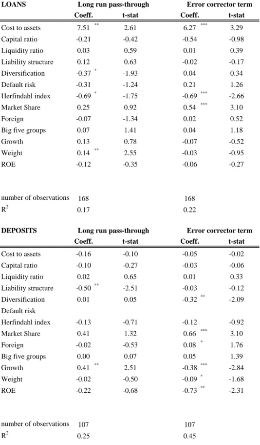
Table 8 summarises the results of the estimation of equation (8) for loans and deposits. It is relevant to keep in mind that the left hand side of the equation is already an estimated value. In addition, observations within a product have some common variance and by pooling over products each observation gets some product speci…c variance. For these reasons, the homoescedasticity
condition is violated. To deal with this issue, we compute heteroscedasticity- consistent standard errors as suggested by White (1980). Moreover, the error correction term takes always negative values, implying that negative estimated coe¢ cients for the explanatory variable contribute to increase the error correction term resulting in a faster pass-through.
In general, results are statistically more signi…cant for deposits than for loans. This may result from the fact that it is more di¢ cult to understand the setting of loan’s interest rates as problems of assimetry of information are more important than for deposits. In any case, given the small number of observations, results should be used with caution.
Capital and liquidity ratios are never signi…cant. This …nding strongly contrasts with the results by De Graeve, de Jonghe and Vennet (2004). According to these authors, the capital ratio is "probably the most discerning characteristic" in explaining retail bank interest rate heterogeneity of Belgian banks. The result for Portugal may happen because, in the eighties, there were many restrictions to banking ativities and banks may not have been able to …nd pro…table investments, resulting in an accumulation of capital. In fact, Boucinha e Ribeiro (2008) document that in 1994 capital bu¤ers were close to 80 percent above the minimum capital required. This …gure decreased signi…cantly in 2000 as there was a strong deregulation of banking activities during the nineties. Simultaneously, the convergence in interest rates promoted the rapid increase in credit. However, on average, for the period between 1994 and 2002 capital bu¤ers seem to be signi…cant and, as such, the capital ratio is not a restrictive variable in the behavior of Portuguese banks.
In terms of competition, the concentration of banks across products, measured by the Her…nd-ahl index, proves to be relevant to explain interest rate heterogeneity in loan but not deposit retail rates. Results show that for products where concentration is higher, the speed of adjustment in changes in interbank rates is higher but the long run pass-through is less complete. In turn, market share is relevant to explain the speed of adjustment of both loan and deposit rates. In this case, we conclude that banks with larger market shares will tend to adjust slower their retail rates than banks with smaller market shares. This result is in line with the relative market power hypothesis of Berger (1995). There is no evidence on the alternative hypothesis, that is, that banks with more operational e¢ ciency would tend to pass its e¢ ciency advantage on to their customers. In fact, results are mixed for loans as banks with higher cost to assets ratios adjust loan interest rates at a slower rate but to a more complete pass through than banks with lower cost to assets ratios.
Results on the e¤ect of diversi…cation are mixed. On the one hand, the estimated coe¢ cient of diversi…caton for the error correction term of deposits is signi…cant and negative. This means that more diversi…ed banks adjust deposit interest rates faster than less diversi…ed banks. As the period under study is characterized by decreasing interest rates, this could be interpreted as if banks with more diversi…ed activities were less dependent on deposits and, as such, were able to decrease interest rates on deposits faster than banks more dependent on a more tradicional funding. On the other hand, the long run coe¢ cient for deposits is negative, in line with De Graeve, De Jonghe and Vennet (2004) predictions. As for the liability structure of banks, results on the long run multiplier of deposits are in line with the argument of Berlin and Mester (1999) that banks with a larger share of core deposits are less vulnerable to the evolution of market interest rates. Finally, as in De Graeve, De Jonghe and Vennet (2004), default risk is not a relevant variable to explain loan interest rates pass-through.
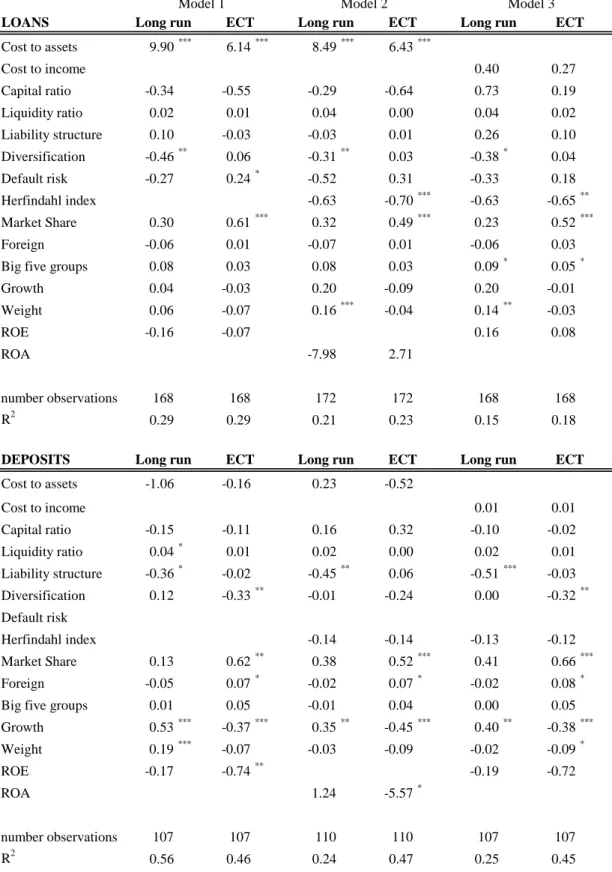
The robustness of the results has been checked in several ways (Table 9). The …rst test was to introduce one dummy variable per product instead of the Her…ndahl index. This case corresponds to Model 1 in Table 9. The main conclusions still apply. A second test consisted in using the concentration index C4 instead of the Her…ndahl index. Results are not reported as they are very similar to the ones in Table 8. Robustness tests were performed using alternative de…nitions of some explanatory variables. For instance, a return on assets ratio (ROA) was used instead of the return on equity (ROE) as a measure of pro…tability (Model 2 in Table 9). In this case,
diversi…cation e¤ect is no longer relevant to explain the speed of adjustment of deposits interest rate. A fourth robustness test consisted in replacing the cost to assets ratio by the cost to income ratio (Model 3 in Table 9). In this case the cost measure is no longer relevant to explain the behavior of the loan interest rates.
An alternative formulation including a measure of default risk in the long term model for loans was also considered. This formulation results in a positive and signi…cant coe¢ cient of the long term default risk parameter. The long term coe¢ cient of the interbank interest rate decreases although this pattern does not apply to all banks individually. In what concerns the determinants of heterogeneity, results are not signi…cantly di¤erent from the ones presented in Table 8.
4
Conclusions
This study addresses the interest rate pass through of the Portuguese banking system. The study is performed along two main questions. First, what are the main characteristics of the interest rate pass through of the Portuguese banking system? Second, does the pass-through of interest rates vary accross banks? In order to answer these questions a data set with quantities and prices set on new operations of loans and deposits was constructed. Data covers information of nine types of loans and six types of deposits for the period between 1990 and 2002. It includes information on products o¤ered to both the corporate sector and households, and also with short term and long term maturities.
Results on the characterization of the interest rate pass through are mostly in line with other published results for the Portuguese banking system. The interest rate pass-through is typically around one for loans and lower than one for deposits. This means that changes in money market rates are fully transmitted to loan rates but not to deposit rates. Regarding the speed of adjust-ment, retail rates of loans to the corporate sector adjust faster to changes in the interbank rate. In addition, we conclude that there is a negative relationship between the maturity and the speed of adjustment for deposit rates while no clear relationship between the maturity and the speed of adjustment emerges for loans.
The availability of micro-level data allows a study on the determinants of the heterogeneity in the pass-through accross banks. The empirical …ndings presented in this work have to be interpreted with caution because the sample period is short and the interest rate cycle covered is limited. Notwithstanding this, some conclusions emerge which seem to be quite robust. First,
Table 8: The determinants of heterogeneity
LOANS
Coeff. t-stat Coeff. t-stat
Cost to assets 7.51 ** 2.61 6.27 *** 3.29 Capital ratio -0.21 -0.42 -0.54 -0.98 Liquidity ratio 0.03 0.59 0.01 0.39 Liability structure 0.12 0.63 -0.02 -0.17 Diversification -0.37 * -1.93 0.04 0.34 Default risk -0.31 -1.24 0.21 1.26 Herfindahl index -0.69 * -1.75 -0.69 *** -2.66 Market Share 0.25 0.92 0.54 *** 3.10 Foreign -0.07 -1.34 0.02 0.52
Big five groups 0.07 1.41 0.04 1.18
Growth 0.13 0.78 -0.07 -0.52 Weight 0.14 ** 2.55 -0.03 -0.95 ROE -0.12 -0.35 -0.06 -0.27 number of observations 168 168 R2 0.17 0.22 DEPOSITS
Coeff. t-stat Coeff. t-stat
Cost to assets -0.16 -0.10 -0.05 -0.02 Capital ratio -0.10 -0.27 -0.03 -0.06 Liquidity ratio 0.02 0.65 0.01 0.33 Liability structure -0.50 ** -2.51 -0.03 -0.12 Diversification 0.01 0.05 -0.32 ** -2.09 Default risk Herfindahl index -0.13 -0.71 -0.12 -0.92 Market Share 0.41 1.32 0.66 *** 3.10 Foreign -0.02 -0.53 0.08 * 1.76
Big five groups 0.00 0.07 0.05 1.39
Growth 0.41 ** 2.51 -0.38 *** -2.84
Weight -0.02 -0.50 -0.09 * -1.68
ROE -0.22 -0.68 -0.73 ** -2.31
number of observations 107 107
R2 0.25 0.45
Notes: The long run coefficient corresponds to b in equation (1) and the error corrector term corresponds toγin equation (2). Standard errors are computed according to White (1980) heteroscedasticity-consistent estimators. * = significance at the 10 per cent level; ** = significance at the 5 per cent level; *** = significance at the 1 per cent level.
Long run pass-through Error corrector term
Table 9: Robustness tests LOANS Cost to assets 9.90*** 6.14*** 8.49*** 6.43*** Cost to income 0.40 0.27 Capital ratio -0.34 -0.55 -0.29 -0.64 0.73 0.19 Liquidity ratio 0.02 0.01 0.04 0.00 0.04 0.02 Liability structure 0.10 -0.03 -0.03 0.01 0.26 0.10 Diversification -0.46** 0.06 -0.31** 0.03 -0.38* 0.04 Default risk -0.27 0.24* -0.52 0.31 -0.33 0.18 Herfindahl index -0.63 -0.70*** -0.63 -0.65** Market Share 0.30 0.61*** 0.32 0.49*** 0.23 0.52*** Foreign -0.06 0.01 -0.07 0.01 -0.06 0.03
Big five groups 0.08 0.03 0.08 0.03 0.09* 0.05*
Growth 0.04 -0.03 0.20 -0.09 0.20 -0.01 Weight 0.06 -0.07 0.16*** -0.04 0.14** -0.03 ROE -0.16 -0.07 0.16 0.08 ROA -7.98 2.71 number observations 168 168 172 172 168 168 R2 0.29 0.29 0.21 0.23 0.15 0.18 DEPOSITS Cost to assets -1.06 -0.16 0.23 -0.52 Cost to income 0.01 0.01 Capital ratio -0.15 -0.11 0.16 0.32 -0.10 -0.02 Liquidity ratio 0.04* 0.01 0.02 0.00 0.02 0.01 Liability structure -0.36* -0.02 -0.45** 0.06 -0.51*** -0.03 Diversification 0.12 -0.33** -0.01 -0.24 0.00 -0.32** Default risk Herfindahl index -0.14 -0.14 -0.13 -0.12 Market Share 0.13 0.62** 0.38 0.52*** 0.41 0.66*** Foreign -0.05 0.07* -0.02 0.07* -0.02 0.08*
Big five groups 0.01 0.05 -0.01 0.04 0.00 0.05
Growth 0.53*** -0.37*** 0.35** -0.45*** 0.40** -0.38*** Weight 0.19*** -0.07 -0.03 -0.09 -0.02 -0.09* ROE -0.17 -0.74** -0.19 -0.72 ROA 1.24 -5.57* number observations 107 107 110 110 107 107 R2 0.56 0.46 0.24 0.47 0.25 0.45
Notes: The long run coefficient corresponds to b in equation (1) and the error corrector term corresponds toγin equation (2). Model 1 considers product dummies; Model 2 replaces the ROE measure by ROA and Moodel 3 replaces the cost to assets ratio by the cost to income ratio. * = significance at the 10 per cent level; ** = significance at the 5 per cent level; *** = significance at the 1 per cent level.
ECT
Model 1 Model 2 Model 3
Long run ECT Long run ECT Long run ECT
liquidity and capital ratios do not seem relevant for the determination of the speed and long run pass-through. In the case of the capital ratio, this could be due to the fact that capital ratios of Portuguese banks were still relatively high during the 90’s, following a period of many constraints in banking activities which prevented banks from allocating capital to pro…table investments. Second, banks with higher market shares are shown to adjust both loan and deposit interest rates at a slower speed than banks with lower market shares. However, the e¤ect of market share occurs only in the short-term as this variable is not relevant to explain the long-run coe¢ cients.
For further research, it would be interesting to investigate if there is any evidence that within a bank the speed of adjustment and the pass through is di¤erent accross products. To analyse this question, it would be necessary to have a more balanced panel. In this work, only a very small number of banks is operating in several of the products considered. Another extension would be to construct a longer time-series in order to consider a complete business cycle. There is some
evidence that the degree of price stickiness is likely to be assymetric over the interest rate cycle. This analysis is not possibe to perform with the data available as it only captures a period of decreasing interest rates.
References
Banco de Portugal, 1999, Annual Report, Box II.7.2
Berger, A., 1995, The Pro…t-Structure RElationship in Banking - Tests of Market-Power and E¢ cient-Structure Hypotheses, 27, p. 404-431.
Berlin, M. and Mester, L., 1999, Deposits and Relationship Lending, Review of Financial Studies, 12, p. 579-607.
Boucinha, M, and Ribeiro, N, 2008, Determinantes do Excesso de Capital dos Bancos Por-tugueses, Financial Stability Report 2007
Breitung, 2000, The Local Power of Some Unit Root Tests for Panel Data, in: B. Baltagi (ed.), Nonstationary Panels, Panel Cointegration, and Dynamic Panels, Advances in Econometrics, Vol. 15, JAI: Amsterdam, 2000, p. 161-178.
Cottarelli, C. and Kourelis, A. 1994, Financial Structure, Bank Lending Rates and the
Trans-mission Mechanism of Monetary Policy, IMF Sta¤ Papers, 41(4), p. 587-623.
De Bondt, G., 2002, Retail rate interest rate pass-through: new evidence at the euro area level, European Central Bank Working Paper Series, n. 136.
De Bondt, G., Mojon, B. and Valla, N., 2005, Term structure and the sluggishness of retail bank interest rates in euro area countries, European Central Bank Working Paper Series, n. 518. De Graeve, F., de Jonghe, O. and Vennet, R. V., 2004, The Determinants of Pass-Through of Market Conditions to Bank Retail Interest Rates in Belgium, National Bank of Belgium Working Paper Serie, n. 47.
Dickey, D. A. and Fuller, W. A., 1979, Distribution of the Estimators for Autoregressive Time Series with a Unit Root, Journal of the American Statisticas Association, 74, p. 427-31.
Donnay, M. and Degryse, H., 2001, Bank Lending Rate Pass-Through and Di¤erences in the Transmission of a Single EMU Monetary Policy, Discussion Paper, Center for Economic Studies, K.U. Leuven, 01.17
ECB, 2002, Report on Financial Structures, Frankfurt Am Main, European Central Bank. Fuertes, A. and He¤ernan, S.A., 2006, Interest Rate Transmission in the UK: A Comparative Analysis Across Financial Firms and Products, International Journal of Finance and Economics, Forthcoming [Available at SSRN]
Hadri, K., 2000, Testing for Stationarity in Heterogeneous Panel Data, Econometrics Journal, 3, p. 148-161.