An Implementation of Fully Convolutional Network for Surface Mesh Segmentation

University of Wisconsin Milwaukee University of Wisconsin Milwaukee

UWM Digital Commons

UWM Digital Commons

Theses and Dissertations

December 2019

An Implementation of Fully Convolutional Network for Surface

An Implementation of Fully Convolutional Network for Surface

Mesh Segmentation

Mesh Segmentation

University of Wisconsin-Milwaukee

Follow this and additional works at: https://dc.uwm.edu/etd Part of the Computer Sciences Commons

Recommended Citation Recommended Citation

Zhang, Taiyu, "An Implementation of Fully Convolutional Network for Surface Mesh Segmentation" (2019). Theses and Dissertations. 2341.

https://dc.uwm.edu/etd/2341

This Thesis is brought to you for free and open access by UWM Digital Commons. It has been accepted for inclusion in Theses and Dissertations by an authorized administrator of UWM Digital Commons. For more information, please contact [email protected].

AN IMPLEMENTATION OF FULLY CONVOLUTIONAL

NETWORK FOR SURFACE MESH SEGMENTATION

by

Taiyu Zhang

A Thesis Submitted in

Partial Fulfillment of the

Requirements for the Degree of

Master of Science

in Computer Science

at

The University of Wisconsin Milwaukee

December 2019

ii

ABSTRACT

AN IMPLEMENTATION OF FULLY CONVOLUTIONAL NETWORK FOR

SURFACE MESH SEGMENTATION

by Taiyu Zhang

The University of Wisconsin Milwaukee, 2019 Under the Supervision of Professor Zeyun Yu

This thesis presents an implementation of a 3-Dimensional triangular surface mesh segmentation architecture named Shape Fully Convolutional Network, which is proposed by Pengyu Wang and Yuan Gan in 2018. They designed a deep neural network that has a similar architecture as the Fully Convolutional Network, which provides a good segmentation result for 2D images, on 3D triangular surface meshes. In their implementation, 3D surface meshes are represented as graph structures to feed the network. There are three main barriers when applying the Fully Convolutional

Network to graph-based data structures.

• First, the pooling operation is much harder to apply to general graphs. • Second, the convolution order on a graph structure is unstable.

• _{Third, the raw data of surface meshes cannot be directly applied to the network.} To solve these problems, first, all the nodes inside the graph are re-ordered into a 1-dimensional list based on a multi-level graph coarsening algorithm, which allows the pooling operation to be applied as easily as a 1D pooling. Second, a self-defined generating layer is added before each convolution layer in the network to generate the neighbors of each node on the graph, and at the same time, sort all neighbors based on

iii

the L2 similarity to keep the convolution operation in a stable manner. Finally, three translation and rotation free low-level geometric features are pre-processed and used as input to train the network. This Shape Fully Convolution Network can effectively learn and predict triangular face-wise labels. In the end, to achieve a better result, the final labeling is optimized by the multi-label graph cut algorithm, which gives punishment to the predicted result based on the smoothness of the surface. The experiments show that the model can effectively learn and predict triangle-wise labels on surface meshes and yields good segmentation results.

iv

TABLE OF CONTENTS

ABSTRACT... ii

TABLE OF CONTENTS ... iv

LIST OF FIGURES ... vi

LIST OF TABLES ... viii

1. Introduction ... 1

2. Related Work ... 5

2.1. Fully Convolutional Network ... 5

2.2. Graphs Convolutional Neural Network... 5

2.3. Deep Learning on 3D Shapes ... 6

3. Shape Fully Convolutional Network ... 8

3.1. Pooling Operation ... 8

3.1.1. Multi-level Graph Coarsening ... 9

3.1.2. Fast pooling based on coarsening ... 10

3.1.3. Pooling on 3D Surface Mesh ... 12

3.2. Convolution Operation ... 14 3.2.1. Generating Neighborhood ... 15 3.2.2. Convolution Order ... 15 3.3. SFCN Architecture ... 16 3.3.1. Input Data ... 17 3.3.2. Generating Layer ... 18 3.3.3. Convolution Layer ... 19 3.3.4. Pooling Layer ... 20 3.3.5. Deconvolution Layer ... 21

v

3.3.6. The SFCN Architecture ... 23

4. Features on 3D Polygon Mesh ... 26

4.1. Geodesic Distance ... 27

4.2. Shape Context ... 28

4.3. Spin Image ... 31

5. Post Optimization ... 36

5.1. Finding the Optimal Swap Move ... 37

6. Experiment Result ... 40

6.1. Data ... 40

6.2. Shape Fully Convolution Network Parameters ... 40

6.3. Computation Time... 40 6.4. Result ... 41 6.4.1. Chairs Dataset ... 41 6.4.2. Vases Dataset ... 43 6.5. Limitations ... 45 7. Conclusion ... 46 References ... 47

vi

LIST OF FIGURES

Figure 1 The pipeline of the Shape Fully Convolutional Network model ... 4

Figure 2 Overview of the Multilevel Coarsening ... 9

Figure 3 Example of coarsening output ... 11

Figure 4 Example of Graph Coarsening and Pooling ... 12

Figure 5 Negative log plot ... 13

Figure 6 Convert mesh to general graph ... 14

Figure 7 Convolution process on a shape ... 15

Figure 8 Generating Layer ... 18

Figure 9 2-D Convolution Operation [4] ... 19

Figure 10 The convolution operation after generating layer ... 20

Figure 11 Pooling operation ... 21

Figure 12 Image-based deconvolution operation ... 22

Figure 13 Deconvolution operation in SFCN ... 23

Figure 14 The SFCN Architecture for a single input sample ... 25

Figure 15 Examples of the distribution of the average geodesic distance ... 28

Figure 16 Shape context computation and matching ... 29

Figure 17 Example of a shape context ... 30

Figure 18 Example of a shape context ... 30

Figure 19 An oriented point basis created at a vertex in a surface mesh ... 31

Figure 20 Spin images for three different oriented points on a surface mesh ... 32

Figure 21 The effect of bin size on the spin image ... 33

vii

Figure 23 The effect of support angle on the spin image ... 34

Figure 24 Example of a spin image ... 35

Figure 25 Example of a spin image ... 36

Figure 26 𝛼𝛼 − 𝛽𝛽 − 𝑠𝑠𝑠𝑠𝑠𝑠𝑠𝑠 algorithm ... 38

Figure 27 An example of the graph 𝐺𝐺𝛼𝛼𝛽𝛽. ... 38

Figure 28 Properties of a cut 𝐶𝐶 on graph 𝐺𝐺𝛼𝛼𝛽𝛽 ... 39

Figure 29 Accuracy plot for 50 test samples in the Chairs dataset ... 41

viii

LIST OF TABLES

Table 1 weight for each edge in 𝐺𝐺𝛼𝛼𝛽𝛽 for 𝑣𝑣 ∈ 𝑉𝑉𝛼𝛼𝛽𝛽 ... 39 Table 2 Visualization of Three samples from the Chairs test set ... 42 Table 3 Visualization of Three samples from the Vases test set ... 44

1

1. Introduction

The concept of segmentation is aiming to divide an object into some meaningful parts so that the internal structure of the object can be revealed. For segmentation on 2D images, labels are assigned to each pixel so the entire image can be divided into several significant components. The same idea is extended to 3D surface meshes. The segmentation on 3D surface meshes is to assign labels to each triangular face and, therefore, achieve the goal of segmentation. These labelings are very helpful in

exploring the inherent characteristic of the shape. As some examples, the segmentation result can be applied to various fields of computer graphics, such as shape editing [1], shape deformation [2], and shape modeling [3]. These make the shape segmentation a research hotspot, but yet tricky in the fields of digital geometric model processing, and instance modeling persist.

Nowadays, the data-driven method, such as deep learning [4], becomes more and more popular in many areas. In the image processing area, convolutional neural networks have shown excellent performance in various image processing problems, such as image classification [5, 6, 7] which aims to predict an image as a whole into some specific classes; and semantic segmentation [8, 9, 10], which aims to predict pixel-wise classes. With the emerging encouraging study results, many researchers have devoted their efforts to various deformation studies on Convolutional Neural Networks. One of which is the Fully Convolutional Network [11]. This network can achieve end-to-end, pixel-to-pixel predictions on semantic image segmentation, with no requirements over the size of input images. Therefore, it has become one of the most

2

popular methods for image segmentation. A couple of variations are build based on the Fully Convolutional Network architecture such as the DeConvNet [12], and U-Net [13]

Although the Fully Convolutional Network [11] can generate good results in 2D image segmentation, it can not be directly applied to 3D surface meshes. This mainly because of three reasons:

• First, unlike the 2D images where the data are stored as a 2D static array, which has a very standard data structure and regular neighborhood relationships. The surface meshes are stored by recording the coordinates for all vertices and the vertex indices for each triangular face. This particular data structure makes the regular pooling and convolution operation hard to apply.

• _{Second, in 2D images, each pixel has a well-organized neighborhood structure} that has a fixed geometric order, where surface meshes do not have similar fixed neighborhood relationships. This un-structured neighborhood ordering may cause the convolution operation to become unstable.

• Third, the RGB data are globally well defined in a 2D image. In other words, a specific color is mapped to the same RGB values across any images. Therefore, it is safe to directly use the RGB value of an image as input data and let the network to figure out the high-level features. On the other hand, the coordinates of vertices or the surface normal of triangular faces are defined locally for each surface mesh, where the translation, such as zoom in and zoom out, and the rotation operation will change the coordinates and face normal for a surface mesh. This makes it unsafe to feed the network directly using the raw data of surface meshes.

3

A novel Shape Fully Convolutional Network [14] is designed based on the Fully Convolutional Network [11] to solve these problems. The Fully Convolutional Network has two main stages: a sampling path and an up-sampling path. The down-sampling path has a similar convolution and pooling architecture compare to the Deep Convolution Neural Network. Inspired by the Graph Convolutional Neural Network [15, 16, 17] where the convolution and pooling operation can be directly applied to an arbitrary graph. The same idea is extended to the Shape Fully Convolutional Network. Based on the design: First, three low-level geometric features are pre-processed and assigned to each triangular face in the surface mesh. Second, the 3D surface mesh is converted to a graph structure with each triangular face as a node and the

neighborhood relationship between two faces as an edge. Third, before feeding the network, the graph is re-ordered into a 1D list based on the multi-level graph coarsening algorithm. Finally, a self-defined generating layer is added in the network before each convolution layer to generate the neighbors for convolution operation.

For the up-sampling path, the transpose-convolution operation proposed by the Fully Convolutional Network [11] is re-used. This operation provides a learnable way to optimize the up-sampling strategy. Moreover, the skip architecture from the Fully Convolutional Network is implemented, which passes the features from the down-sampling path to the up-down-sampling path at each level.

In the end, the prediction from the model is optimized base on a multi-label graph coarsening algorithm, which punishes the predicted labeling with the smoothness of the surface mesh. Figure 1 shows the pipeline of the model:

4

Figure 1 The pipeline of the Shape Fully Convolutional Network model [14]

This Shape Fully Convolution Network is able to train a triangles-to-triangles model for surface mesh segmentation, without any requirements on the triangle numbers of the input shape, and achieve good segmentation results.

5

2. Related Work

2.1. Fully Convolutional Network

The Fully Convolutional Network [11] proposed in 2015 is pioneering research that can effectively solve the problem of semantic image segmentation by pixel-level classification. It uses a down-sampling path that has a similar architecture as the Deep Convolution Neural Network, which is able to extract high-level features from the low-level RGB data. Then an up-sampling path based on the transpose convolution

operating is attached to expand the coarsened features to the original image shape to achieve the pixel-wise prediction. A skip architecture that concatenates the coarsened high-level features in the up-sampling path with the finer low-level features from the down-sampling path is applied to the network to get a better result. Later, a great deal of research has emerged based on the Fully Convolutional Network algorithms and

achieved good results in various fields such as edge detection [18], depth regression [19], optical flow [20], simplifying sketches [21], and etc.. However, the existing research on Fully Convolutional Network is mainly restricted to image processing, largely

because image has a standard data structure, easy for convolution, pooling, and up-sampling operations.

2.2. Graphs Convolutional Neural Network

Standard Convolutional Neural Networks cannot work directly on data which have graph structures. However, there are some previous researches [16, 17, 22, 23] that discussed how to apply Convolutional Neural Networks on graph structures. Some of them [17, 22] use a spectral method by computing bases of the graph Laplacian

6

matrix and perform the convolution in the spectral domain. Where one of the others [16] uses a PATCHY-SAN architecture, which maps from a graph representation onto a vector space representation by extracting locally connected regions from graphs based on a multi-level graph coarsening algorithm.

2.3. Deep Learning on 3D Shapes

The recent researches introduce various methods of deep convolutional

architectures for 3D shapes. By using volumetric representation, which is proposed in the 3D ShapeNet [24] and the volumetric Convolution Neural Network [25], standard 2D convolution and pooling operation, or even augmentation methods can be easily

extended to 3D data. However, data sparsity and the computation cost problem of 3D convolution has not yet been solved. The Projective Convolution Network [26] proposed a multi-view image-based Fully Convolutional Network and a surface-based Conditional Random Fields to do the 3D mesh labeling. Where the RGB data associated with the depth information of each pixel are used as input, however, it may need a lot of time to compute the surface-pixel reference, and more viewpoints to maximally cover the shape surface. Some other methods, such as the Synchronized Spectral Convolutional Neural Network [27] and the Point-net [28] proposed different deep architectures that can be trained directly on point clouds to achieve points segmentation and other 3D points analysis. However, the point cloud structure sampled from the original object surface may lack the intrinsic structure compare to surface mesh. For a better understanding of the intrinsic structures, many types of research directly adapt neural networks to surface meshes. The Geodesic Convolution Neural Network [29] used convolution filters in local

7

geodesic polar coordinates. The Anisotropic Convolutional Neural Network [30] used anisotropic heat kernels as filters. The Mixture Model Convolutional Neural Network [31] considered a more generalized Convolutional Neural Network architecture by using the mixture model.

8

3. Shape Fully Convolutional Network

In 2018, Pengyu Wang and Yuan Gan proposed a 3-dimensional shape segmentation technique named Shape Fully Convolutional Network [14]. In this

architecture, 3D triangular meshes are represented as graph structures with triangular faces as nodes and the neighborhood relationships as edges. Then the graph

convolution and pooling operations proposed in the Graph Convolutional Neural Network [17] are applied to the graph, which is similar to convolutional and pooling operations used on 2D images. The graph is pre-ordered based on the multi-level

coarsening algorithm [17], which allows the pooling operation much more comfortable to apply. Then a bridging function named generating operation [14] is designed that will generate proper neighborhood structures for each face to fit the convolution kernel. After the down-sampling path, the extracted features are then up-sampled using de-convolution operation and skip architecture proposed by the Fully Convolutional

Network [11] that combines the feature from the same stage in the down-sampling path with the output of the de-convolution operation before passing to next stage. Finally, the prediction is optimized based on the multi-level graph cut algorithm [32].

3.1. Pooling Operation

Apply general convolution and pooling operation to graphs is not straightforward, because the general convolution and pooling are designed only for grid structures such as images. The major obstacles of applying them are to figure out the pooling order and convolution order. The pooling operation requires meaningful neighborhoods on graphs, where similar nodes are clustered together. However, finding out multiple levels of

9

clustering is equivalent to finding out the multi-scale clustering of the graph, which is known as NP-hard [33]. Therefore, apply an approximation algorithm is much more practical.

3.1.1. Multi-level Graph Coarsening

To accurately approximate the multi-scale clustering, the coarsening phase proposed by the Graclus multilevel clustering algorithm [34] is applied, which has shown to be extremely efficient at clustering a large variety of graphs. Assume an input graph

𝐺𝐺0(𝑉𝑉0,𝐸𝐸0) with a set of vertices 𝑉𝑉0 and a set of edges 𝐸𝐸0 where each edge between two

vertices represents their similarity. The goal for this coarsening phase is to transform the graph 𝐺𝐺0 into a series of smaller and smaller graph 𝐺𝐺1,𝐺𝐺2,⋯,𝐺𝐺𝑚𝑚 such that |𝑉𝑉0| > |𝑉𝑉1| >⋯ > |𝑉𝑉𝑚𝑚|. The overview of multi-level coarsening is shown in figure 2.

10

For each level 𝑖𝑖, the algorithm is as follows: Start with all vertices un-marked. Visit each un-marked vertex 𝑢𝑢 ∈ 𝑉𝑉𝑖𝑖 in random order, search for another unmarked vertex 𝑣𝑣 ∈

𝑛𝑛𝑛𝑛𝑖𝑖𝑛𝑛ℎ𝑏𝑏𝑏𝑏𝑏𝑏(𝑢𝑢) such that 𝑢𝑢 and 𝑣𝑣 corresponds to the highest normalized weight

𝑠𝑠(𝑢𝑢,𝑣𝑣) =𝑛𝑛_𝑑𝑑(𝑢𝑢_(𝑢𝑢,𝑣𝑣_{) +}) 𝑛𝑛_𝑑𝑑(𝑢𝑢_(𝑣𝑣,𝑣𝑣₎)

among all neighbors. Then merge 𝑢𝑢 and 𝑣𝑣, and set them as marked. If all neighbors of 𝑢𝑢

have been marked, only mark 𝑢𝑢 and do not merge it. In the equation, 𝑛𝑛(𝑢𝑢,𝑣𝑣)

corresponds to the edge weight between 𝑢𝑢 and 𝑣𝑣. The higher the weight of the edge, the more likely the corresponding vertices would be clustered tighter. This edge weight should be normalized by 𝑑𝑑(𝑢𝑢), and 𝑑𝑑(𝑣𝑣), which are the degrees of vertex 𝑢𝑢 and 𝑣𝑣. The degree of vertex 𝑢𝑢 is defined as the summation of edge weights between 𝑢𝑢 and all its neighbors

𝑑𝑑(𝑢𝑢) = � 𝑛𝑛(𝑢𝑢,𝑣𝑣) 𝑣𝑣 ∈ 𝑛𝑛𝑛𝑛𝑖𝑖𝑛𝑛ℎ𝑏𝑏𝑏𝑏𝑏𝑏(𝑢𝑢)

If 𝑑𝑑(𝑢𝑢) is low, it means that vertex 𝑢𝑢 is unique in its neighborhood. It tends to not cluster with any neighbor. On the other hand, if 𝑑𝑑(𝑢𝑢) is high, it means that vertex 𝑢𝑢 is similar to its neighborhood, and it can be clustered with more of its neighbors. By normalizing the edge weight by the degrees of the corresponding vertices, the coarsening algorithm can be applied to more general graphs.

3.1.2. Fast pooling based on coarsening

After coarsening, the vertices of the graph and its coarsened versions are not arranged in a way that pooling operation can be easily applied. However, it is possible to arrange the vertices such that a graph pooling operation can be as efficient as the 1D

11

pooling. The output of the coarsening algorithm should be a binary tree with each parent corresponds to the merged nodes from its children. Each node would have either two children if it was matched at the finer level, or one, if it was not. Figure 3 shows an example of coarsening process and output. Suppose we carry out two layers of

clustering. The original graph has 8 nodes. Then during the first clustering, node 4 and node 7 are leftover as singleton nodes. Therefore, node 2 and node 4 in layer 2 have only one child. During the second clustering, node 1 and node 2 are clustered together, and node 3 and node 4 are clustered together. Node 0 is leftover as a singleton, and therefore, node 0 in the base layer only has one child.

Figure 3 Example of coarsening output [17]

To get the proper pooling order, we need to re-arrange the tree structure

returned from the coarsening phase into a balanced binary tree. From the base level to input level (coarsest level to finest level), fake nodes (disconnected nodes) are added to pair with the singletons so that each node should have two children:

1) regular nodes either have two regular nodes as children, 2) or one singleton and a fake node as children.

12

Suppose we carry out two layers of pooling with each pooling of size 2. Then two coarsening operations are needed. Based on figure 3, we then need to add fake nodes to make sure the output is a balanced binary tree. Figure 4 shows the pooling process and output.

Figure 4 Example of Graph Coarsening and Pooling. [17]

All fake nodes added are initialized with neutral values, such as 0 if the network uses the Rectified Linear Unit (ReLU) as activation function and the max-pooling. The ReLU activation will not react in backpropagation if the feature value is 0, and the max-pooling will always filter the fake nodes off.

3.1.3. Pooling on 3D Surface Mesh

The multi-level graph coarsening algorithm can re-arrange the original graph, which can make the pooling operation very efficient. But our goal is to apply the Fully Convolutional Network [11] on 3D surface meshes with each triangular face has a label. Therefore, we must convert the surface mesh into a graph structure with each node represent a triangular face on the mesh. We also need to set up proper edge weights between two neighborhood faces. The edge weight should be significantly large if the

13

two corresponding faces tend to cluster together, or significantly small otherwise. In surface mesh, two faces are considered similar if the two faces tend to fit in the same plane. In other words, two faces are considered similar if the dihedral angle between the two faces is close to 180°. Therefore, we can define the edge weights 𝑠𝑠(𝛼𝛼,𝛽𝛽) between two neighborhood faces 𝛼𝛼 and 𝛽𝛽 as:

𝑠𝑠(𝛼𝛼,𝛽𝛽) =−log (𝜃𝜃_𝜋𝜋+𝜖𝜖)

Where 𝜃𝜃 is the angle between two face normal in radian

𝜃𝜃= arccos{𝑛𝑛�⃗(𝛼𝛼)⋅ 𝑛𝑛�⃗(𝛽𝛽)}

so that the dihedral angle 𝜔𝜔 =𝜋𝜋 − 𝜃𝜃. The constant 𝜖𝜖 is the smallest float number to avoid 𝑙𝑙𝑏𝑏𝑛𝑛 zero problems. And face normal should be three-dimensional unit vectors.

Figure 5 𝑠𝑠(𝛼𝛼,𝛽𝛽) will be significantly large if 𝜃𝜃 is close to 0 (dihedral angle between the two faces is close to 180°)

Now the original surface mesh, like figure 6 (b), can be represented by a graph

𝐺𝐺(𝑉𝑉,𝐸𝐸,𝑊𝑊), as shown in figure 6 (c), with vertices 𝑉𝑉 represents all the triangular faces, edge 𝐸𝐸 represents the neighborhood relationship, and edge weight 𝑊𝑊 represents the tendency of clustering.

14

Figure 6 (a) Image data representation; (b) surface mesh representation; (c) surface mesh represented as graph structure [14]

The entire multi-level coarsening algorithm then can be described as a function that takes a graph 𝐺𝐺 as an argument, the number of levels as a parameter and returns a list of coarsened graphs and a permutation vector which can permute the original faces vector for fast pooling:

𝑐𝑐𝑏𝑏𝑠𝑠𝑏𝑏𝑠𝑠𝑛𝑛𝑛𝑛𝑖𝑖𝑛𝑛𝑛𝑛(𝐺𝐺,𝑙𝑙𝑛𝑛𝑣𝑣𝑛𝑛𝑙𝑙= 10)→([𝐺𝐺0⋯ 𝐺𝐺𝑚𝑚],𝑠𝑠𝑛𝑛𝑏𝑏𝑝𝑝)

If 5 pooling operation of size (4, 1) is applied in the network, then 10 levels of

coarsening are required because each level only reduces the number of nodes to half of its original amount.

3.2. Convolution Operation

The coarsening operation provides a way to permute the original graph into an order that pooling can be comfortably applied. However, the convolution operation requires a more structured neighborhood relationship and ordering. The graph built from a surface mesh has neighborhood relationships, just like an image. But the irregularity of the neighborhood structure restrains it from being directly represented and applied to

15

the convolution operation. Therefore, restructuring the graph representation is necessary.

3.2.1. Generating Neighborhood

In order to re-construct the graph for convolution operation, each triangular face is viewed as a source node, and the breadth-first graph search is applied to generate a set of 𝐾𝐾 nodes (a source node associated with 𝐾𝐾 −1 neighbors), as shown in figure 7 (a) and (b). Then based on the generated neighborhood structure, like figure 6 (c), a convolution kernel of shape (1,𝐾𝐾) can be easily applied.

Figure 7 Convolution process on a shape [14]. (a) surface mesh represented as a graph; (b) the neighborhood nodes of different sources after breadth-first graph search; (c) convolution order of each neighborhood set.

Since a convolution operation is needed after each pooling, we have to

determine the neighbors of the coarsened graph after each pooling stage. To achieve this, we need to apply a neighborhood search on each graph returned from the

coarsening algorithm.

3.2.2. Convolution Order

Another problem when process convolution operation is the convolution order. When performing the convolution operation on an image, it is easy to determine the

16

order of the convolution according to the spatial arrangement of the pixels. But it is rather challenging to determine the spatial orders amount the 3-dimensional surface mesh. Hence, sorting is applied after the neighborhood generation. Sorting ensures that the elements in each neighborhood set can be convolved by the same rules, so the convolution operation can better activate features. In this work, the neighbors are sorted based on the L2 similarity in the input feature space. Suppose an input data has a 4-dimensional shape as (𝑠𝑠𝑠𝑠𝑝𝑝𝑠𝑠𝑙𝑙𝑛𝑛𝑠𝑠,𝑓𝑓𝑠𝑠𝑐𝑐𝑛𝑛𝑠𝑠,𝑛𝑛𝑛𝑛𝑖𝑖𝑛𝑛ℎ𝑏𝑏𝑏𝑏𝑏𝑏𝑠𝑠,𝑓𝑓𝑛𝑛𝑠𝑠𝑓𝑓𝑢𝑢𝑏𝑏𝑛𝑛𝑠𝑠). In the neighborhood dimension, the first element is always the current source node. All elements after it are neighbors of the source node. The purpose is to keep the source node as the first element and sort all its neighbors based on the L2 similarity between the source node and the neighbor node.

𝐿𝐿2 = (𝑛𝑛𝑛𝑛𝑖𝑖𝑛𝑛ℎ𝑏𝑏𝑏𝑏𝑏𝑏[𝑖𝑖]− 𝑛𝑛𝑛𝑛𝑖𝑖𝑛𝑛ℎ𝑏𝑏𝑏𝑏𝑏𝑏[0])2, 𝑖𝑖 ∈[1,𝑛𝑛𝑢𝑢𝑝𝑝𝑏𝑏𝑓𝑓𝑛𝑛𝑛𝑛𝑖𝑖𝑛𝑛ℎ𝑏𝑏𝑏𝑏𝑏𝑏𝑠𝑠]

If more than one feature is presented, then the summation of the L2 similarity for all features is used to sort the neighbors.

3.3. SFCN Architecture

After reconstructing the graph so that pooling and convolution operations can be easily applied, a Shape Fully Convolution Network then designed to process the

segmentation task. First, reconstruct the data using the multi-level coarsening and breadth-first neighborhood searching algorithm. Then apply the Fully Convolutional Network [11] using convolution kernel of (1,𝑛𝑛+ 1), pooling size of (4, 1), and

deconvolution kernel of (4, 1) with stride (4, 1). where 𝑛𝑛 denotes the neighborhood size of each face.

17

3.3.1. Input Data

First, a graph 𝐺𝐺(𝑉𝑉,𝐸𝐸,𝑊𝑊) is created based on the face adjacency relationship of a surface mesh 𝑀𝑀. Where 𝑉𝑉 is a set of faces on the mesh, 𝐸𝐸 is a set of adjacent faces, and 𝑊𝑊 is the set of weights calculated based on the dihedral angle between two

adjacent faces. Then the multi-level coarsening algorithm is applied to the graph to get the pooling order. The algorithm will return a list of coarsened graphs and a permutation vector 𝑃𝑃 which can re-organize the original data into an order that pooling can be easily applied.

([𝐺𝐺0⋯ 𝐺𝐺9],𝑃𝑃) ← 𝑐𝑐𝑏𝑏𝑠𝑠𝑏𝑏𝑠𝑠𝑛𝑛𝑛𝑛𝑖𝑖𝑛𝑛𝑛𝑛(𝐺𝐺,𝑙𝑙𝑛𝑛𝑣𝑣𝑛𝑛𝑙𝑙= 10)

The breath-first search algorithm is then applied to the coarsened graph 𝐺𝐺𝑖𝑖 with 𝑖𝑖 ∈

𝑛𝑛𝑣𝑣𝑛𝑛𝑛𝑛𝑛𝑛𝑢𝑢𝑏𝑏𝑛𝑛𝑏𝑏 to match the pooling size of 4.

[𝑁𝑁0⋯ 𝑁𝑁4]← 𝑏𝑏𝑏𝑏𝑛𝑛𝑠𝑠𝑓𝑓ℎ_𝑓𝑓𝑖𝑖𝑏𝑏𝑠𝑠𝑓𝑓_𝑠𝑠𝑛𝑛𝑠𝑠𝑏𝑏𝑐𝑐ℎ([𝐺𝐺0,𝐺𝐺2,𝐺𝐺4,𝐺𝐺6,𝐺𝐺8])

𝑁𝑁𝑖𝑖 should have the shape as (𝑝𝑝𝑖𝑖,𝑛𝑛) with 𝑝𝑝𝑖𝑖 denotes the number of nodes in the graph

𝐺𝐺𝑖𝑖 and 𝑛𝑛 denotes the neighbor size. At the same time, the original input data with shape

as (𝑓𝑓,𝑐𝑐) are permuted based on the permutation vector 𝑃𝑃 in the first dimension. The result after permutation should have the shape as (ℎ,𝑐𝑐) where ℎ represents the number of nodes of the base graph 𝐺𝐺0 after adding all the fake notes. Finally, the permuted

result is reshaped to 3-dimensional data with shape (h, 1, c) and use as input data to the network.

18

3.3.2. Generating Layer

The Shape Fully Convolutional Network [14] includes a generating layer before each convolution layer to process the convolution operation properly. First, as shown in Figure 8 (a), the input data are pre-permuted based on the permutation vector

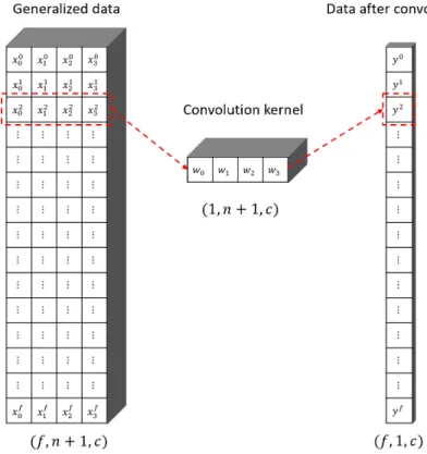
calculated from the multi-level coarsening algorithm. Second, the neighborhood indices, as shown in Figure 8 (b), are pre-calculated by the breadth-first graph search algorithm, and the neighbors are sorted based on the L2 similarity between the source node and each of its neighbor. Finally, the original data and the neighbors are concatenated together in the neighbor dimension makes the output has the shape as (𝑓𝑓,𝑛𝑛+ 1,𝑐𝑐), as shown in Figure 8 (c), where each row is sequenced in the convolution order represents a neighborhood set of 𝑛𝑛+ 1 nodes. By storing data in this way, we can achieve the convolution operation by row and pooling operation by column.

Figure 8 Generating Layer [14]. (a) the permutation vector, the nodes in blue represent true node on the graph, nodes in the red are fake nodes. (b) neighborhood set of each node, data represent the offset of each node. (c) outputs of

the generating layer, where the convolution operation can be applied by row, and the pooling operation can be applied by column.

19

3.3.3. Convolution Layer

The name “convolution” indicates that the layer employs a mathematical

operation called convolution. Convolution is a specialized kind of linear operation. In the implementation, instead of setup each unit inside a layer as a set of weights to all

features of input data, we consider each unit as a filter (kernel), which has much fewer parameters but will be shared by all features. The convolution layer designed for the graph follows the same rule as to apply the convolution operation on 2D-images, which are shown in Figure 9.

Figure 9 2-D Convolution Operation [4]

The output shape (𝐻𝐻𝑏𝑏𝑢𝑢𝑜𝑜,𝑊𝑊𝑏𝑏𝑢𝑢𝑜𝑜) can be calculated by the equations as follow:

𝐻𝐻𝑏𝑏𝑢𝑢𝑜𝑜 =�𝐻𝐻𝑖𝑖𝑛𝑛+ 2_𝑠𝑠𝑠𝑠𝐻𝐻− 𝑓𝑓𝐻𝐻

𝐻𝐻 + 1�

𝑊𝑊𝑏𝑏𝑢𝑢𝑜𝑜 =�𝑊𝑊𝑖𝑖𝑛𝑛+ 2_𝑠𝑠𝑠𝑠𝑊𝑊− 𝑓𝑓𝑊𝑊

20

Where (𝐻𝐻𝑖𝑖𝑛𝑛,𝑊𝑊𝑖𝑖𝑛𝑛) represent the shape of input to the convolution layer. 𝑠𝑠𝐻𝐻 and 𝑠𝑠𝑊𝑊

represent the vertical and horizontal padding. 𝑠𝑠𝐻𝐻 and 𝑠𝑠𝑊𝑊 represent the vertical and

horizontal stride. And (𝑓𝑓𝐻𝐻,𝑓𝑓𝑊𝑊) is the shape of the filter.

As discussed in section 4.2.1, the generating layer will distribute the data into shape (𝑓𝑓,𝑛𝑛+ 1,𝑐𝑐). Then a convolution layer with (1,𝑛𝑛+ 1,𝑐𝑐) is then applied to it. We use no padding [(𝑠𝑠𝐻𝐻,𝑠𝑠𝑊𝑊) = (0, 0)] and single strides [(𝑠𝑠𝐻𝐻,𝑠𝑠𝑊𝑊) = (1, 1)]. Based on the

equation, we can get the output shape as (𝑓𝑓, 1,𝑐𝑐), as shown in Figure 10.

Figure 10 The convolution operation after generating layer, the subscriptions represent the neighbor dimension indices, and the superscriptions represent the face dimension indices.

3.3.4. Pooling Layer

A pooling layer is usually added after the convolution layer to reduce the size of the representation. At the same time, the pooling layer can kind of “highlight” the

21

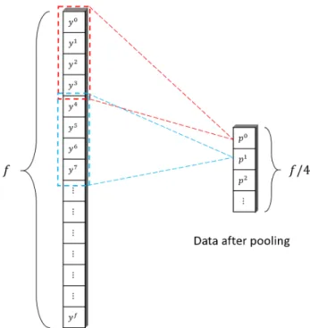
important information after convolution in case of speed up the calculation and make the feature detection more robust. In the Shape Fully Convolution Network, a max-pooling with shape (4, 1) and stride (4, 1) is applied after each convolution layer, which reduces the face dimension to a quarter of its original representation, as shown in Figure 11. Because all the fake nodes added have 0 as their features and all those zeros have no effect on the networks because of the Rectified Linear Unit (ReLU) activation.

Therefore, by using max-pooling, the output will always be the most significant real nodes or fake node if all four of its original inputs are fake.

Figure 11 Pooling operation where 𝑠𝑠0_{=𝑝𝑝𝑠𝑠𝑚𝑚 (𝑦𝑦}0_,𝑦𝑦1_,𝑦𝑦2_,𝑦𝑦3_{), 𝑠𝑠}2_{=𝑝𝑝𝑠𝑠𝑚𝑚 (𝑦𝑦}4_,𝑦𝑦5_,𝑦𝑦6_,𝑦𝑦7_{), and etc.}

3.3.5. Deconvolution Layer

Like the Fully Convolutional Network [11], the Shape Fully Convolutional Network [14] architecture still needs the expansive path before the output layer to achieve the

22

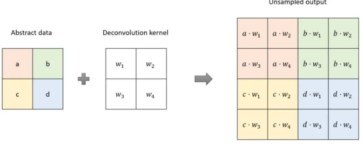
pixel-wise or triangular face wise prediction. There are several ways to process up-sampling. In the Fully Convolutional Network [11], a learnable up-sampling strategy named deconvolution operation or transpose convolution operation is applied to allow the network itself to figure out the optimal up-sampling through backward-propagation. The idea is the same as convolution operation but in an inversed way. Figure 12 shows the details of the deconvolution operation

Figure 12 Image-based deconvolution operation with filter shape (2, 2) and stride (2, 2)

In the Shape Fully Convolutional Network [14], the deconvolution layer can also be used to up-sample the data. As described previously, the SFCN regards pooling as a graph coarsening by clustering 4 vertices. Therefore, it is easy to reuse the image-based deconvolution implementation in the Fully Convolutional Network [11]. The

difference is that the width of the deconvolutional kernel in the original FCN architecture is changed to 1, and the height and stride are set to the pooling size, which is 4. Figure 13 shows the details about the deconvolution operation in SFCN.

23

Figure 13 Deconvolution operation in SFCN with kernel size (4, 1) and stride (4, 1)

3.3.6. The SFCN Architecture

The Shape Fully Convolutional Network [14] is an architecture that combines all the layers discussed above. Figure 14 shows the detailed SFCN structure with a single sample as input. It includes five stages in the down-sampling path and five stages in the up-sampling or expansive path. The input data should be a four-dimensional matrix with shape as (𝑠𝑠,𝑓𝑓, 1,𝑐𝑐), where 𝑠𝑠 is the sample size, 𝑓𝑓 is the number of faces per sample, the third dimension is the reserved neighborhood dimension which should be 1 as input, and 𝑐𝑐 is the channel dimension or number of features. It then followed by the down-sampling path that includes five stages with each stage have a generating layer

followed by a convolution layer, then followed by a max-pooling layer. Each generating layer takes two inputs: the original input or the output from previous pooling, and the

24

neighbor indices. It will generate the neighborhood features based on the neighbor indices and concatenate them with the original input, or the pooling output in the

neighborhood dimension, which makes the neighborhood size equals to 𝑛𝑛+ 1, where n is the number of neighbors. After the generating layer, a 2-D convolution layer is applied to the generated data with kernel shape as (1,𝑛𝑛+ 1), single stride, and no padding. Finally, at each stage, a max-pooling of shape (4, 1) is attached after each convolution to high light the extracted features.

For the expansive or up-sampling path, five de-convolution layers are applied with each deconvolution kernel has the shape (4, 1) and stride (4, 1). Also, a skip is applied between the down-sampling path and the up-sampling path at each stage. The skip architecture [11, 35] will combine the coarse, high layer information with the fine, low layer information. Two fully convolution layers are used to connect the down-sampling path and the up-down-sampling path to learning the abstract features. Finally, a SoftMax layer is used as the output layer to predict a probability map for all possible labels of each triangular face.

25

Figure 14 The SFCN Architecture for a single input sample

gen1:(f,n,c) gen3:(f/16,n,128) gen5:(f/256,n,512) [up2,pool3]:(f/64,1,512) conv1:(f,1,64) conv3:(f/16,1,256), conv5:(f/256,1,1024) [up3,pool2]:(f/16,1,256)

input:(f,1,c) pool1:(f/4,1,64) pool3:(f/64,1,256) pool5:(f/1024,1,1024) [up4,pool1]:(f/4,1,128) out:(f,1,𝑙𝑙) gen2:(f/4,n64) gen4:(f/64,n,256) full1:(f/1024,1,1024) up5:(f,1,32)

conv2:(f/4,1,128) conv4:(f/64,1,512) full2:(f/1024,1,1024)

26

4. Features on 3D Polygon Mesh

In the colored 2D image, the features are the RGB data of each pixel. All the colors are globally well defined so that each specific color is mapped to the same RGB value though out all colored images. Therefore, it is safe to directly use the raw RGB data and let the network itself to figure out the abstract features. However, it is not the case when using 3D polygon mesh as input data. The raw data used to form a 3D polygon mesh usually include the local [𝑚𝑚,𝑦𝑦,𝑧𝑧] coordinatesof each vertex and the vertex indices of each triangular face. Some times the face normal of each face is also recorded. All these pieces of information are defined locally, which means the same object may have different coordinates or different surface normals if it is put in different files with different orientations or different sizes, or if the object is simplified or re-meshed. Hanse, it is not practical to feed the network directly with the raw information of the surface mesh. The features we use to feed the Shape Fully Convolution Network should have two properties:

• _{They should be defined for each triangular face since we treat each face as a} node of the graph

• _{The features should independent with the transformation, rotation, simplification,} and subdivision so that the same object should have relatively the same features with different sizes or different orientations.

There are a lot of features that can be defined to each triangular face and also

independent with the orientation and the size, such as curvature [36], shape diameter function [37], distance from medial surface [38], average geodesic distance [39], shape context [40], and spin image [41]. In this implementation, the average geodesic distance

27

[39], the shape context [40], and the spin image [41] are pre-calculated and combined together as the triangular face wise features to feed the network.

4.1. Geodesic Distance

Geodesic, in definition, is equivalent to the absolute straight line on a curved surface. Geodesic distance is the distance of the straight line on the curved surface between two specific points. Based on the definition, the geodesic distance doesn’t seem necessary to be the shortest path between those two points. However, consider the trade-off between computation cost and accuracy, on a polygon mesh, the shortest path between two points is a good approximation of the geodesic distance between those two points. Therefore, the finer the surface mesh is, the better the approximation can be. It is practical to limit the edge length to be smaller than a threshold.

In the implementation, for each vertex on the mesh, we calculate the shortest path to all other vertices using Dijkstra’s algorithm. This function will return a matrix with shape as (𝑣𝑣,𝑣𝑣) where 𝑣𝑣 represents the number of vertices in the mesh. And each value inside the matrix represents the shortest path from the row index vertex to the column index vertex.

𝑣𝑣𝑛𝑛𝑏𝑏𝑓𝑓𝑛𝑛𝑚𝑚_𝑛𝑛𝑛𝑛𝑏𝑏𝑑𝑑𝑛𝑛𝑠𝑠𝑖𝑖𝑐𝑐(𝑝𝑝𝑛𝑛𝑠𝑠ℎ) → 𝑝𝑝𝑠𝑠𝑓𝑓𝑏𝑏𝑖𝑖𝑚𝑚[𝑣𝑣,𝑣𝑣]

Then, the average geodesic distance is calculated to each vertex by averaging one dimension of the matrix. Finally, the average geodesic distance of each triangular face is approximated by averaging the vertex geodesic distance for three of its vertices. Figure 15 shows the face average geodesic distance on two objects from two different perspectives. We can see that the AGD value is small if close to the center of the object

28

and large if close to the edge. Using the average geodesic distance provides rotation invariance shape descriptor. Normalize the average geodesic distance for each surface mesh to between [0, 1] can make it also translation invariant.

(a) (b)

(c) (d)

Figure 15 Examples of the distribution of the average geodesic distance, (a), (b) two perspectives of a chair, (c), (d) two perspectives of a candelabra

4.2. Shape Context

The shape context is originally proposed in a 2D shape matching algorithm in 2002 with each object as a point set [40]. To see whether two shapes can be matched with each other, some kinds of shape descriptor is needed for the comparison. The

29

initial idea is to use the vector originating from a point to all other sample points on the shape as a descriptor. Obviously, this will form a matrix with the shape of (𝑛𝑛,𝑛𝑛 −1), where 𝑛𝑛 represent the number of points on the shape. However, since 𝑛𝑛 gets larger, this full set of vectors is much too detailed, and most importantly, consume too much

processing power when using it. The concept of shape context comes above this idea. They propose that the distribution over relative positions of each point is a more robust and compact, yet highly discriminative descriptor.

The shape context is formed as follow: for a point 𝑠𝑠𝑖𝑖 on the shape, compute a

coarse histogram ℎ𝑖𝑖 of the relative coordinates of the remaining 𝑛𝑛 −1 points, where the

bins of the histogram are uniform in log-polar2 _{space, which makes the descriptor more}

sensitive to positions of nearby sample points than to those of points farther away. Figure 16 shows an example.

Figure 16 Shape context computation and matching [40]. (a) and (b) Sampled points. (c) log-polar bins with five bins for 𝑙𝑙𝑏𝑏𝑛𝑛(𝑏𝑏) and 12 bins for 𝜃𝜃. (d), (e), (f) Shape context of three points marked as .(g) correspondences found

30

The similar concept of shape context is applied to 3D triangular meshes with some variance. The geodesic distances from a triangular face to all other vertices are

approximated as described in section 5.1, and 5 logarithmic geodesic distance bins are used. On the other side, 6 uniform angle bins are formed, where angles are measured relative to the normal of each face. This will form a 5 by 6 histogram yielding 30 features total. Figure 17 and Figure 18 show two examples of shape context formed from two faces on two different shapes.

(a)

(b)

(c)

Figure 17 Example of a shape context (a) face select on a mesh of chair, (b) the distribution of all other vertices in

𝑙𝑙𝑏𝑏𝑛𝑛(𝑏𝑏) and angle space, (c) the shape context with 5 𝑙𝑙𝑏𝑏𝑛𝑛 (𝑏𝑏) bins and 6 angle bins.

(a)

(b)

(c)

Figure 18 Example of a shape context (a) face select on a mesh of candelabra, (b) the distribution of all other vertices in 𝑙𝑙𝑏𝑏𝑛𝑛(𝑏𝑏) and angle space, (c) the shape context with 5 𝑙𝑙𝑏𝑏𝑛𝑛 (𝑏𝑏) bins and 6 angle bins.

31

4.3. Spin Image

Spin image is another shape descriptor for shape matching, which is proposed by Andrew E. Johnson in 1999 [41]. The original idea is based on the oriented point cloud object representation, where each point on the object has a surface normal as its direction. If the object representation is a polygon mesh, then the surface normal at a vertex is computed by fitting a plane to the points connected with this vertex. An oriented point can form a partial, object-centered, coordinate system. Two cylindrical coordinates 𝛼𝛼 and 𝛽𝛽 are defined respect to the oriented point. 𝛼𝛼 defined as the

perpendicular distance to the line of the surface normal. Since this is the distance from a point to a line, the value should always be positive. 𝛽𝛽 defined as the signed

perpendicular distance to the tangent plane defined by vertex normal and position. This is the distance from a point to a plane. Since the point can be either above or below the plane. The value of 𝛽𝛽 could be either positive or negative. Figure 19 shows an example of an oriented point basis created at a vertex in a surface mesh.

Figure 19 An oriented point basis created at a vertex in a surface mesh [41]

𝛽𝛽 can be calculated by first computing the vector from the origin point to each other vertices, then process the dot product between this vector and the surface normal.

32

where 𝑚𝑚 and 𝑠𝑠 are 3D coordinates of the vertex, and 𝑛𝑛�⃗ is the surface normal unit vector. Since the surface normal is a unit vector, the dot product of the two vectors will return the projection of the (���������������⃗𝑚𝑚 − 𝑠𝑠) vector on 𝑛𝑛�⃗ direction, where if 𝑚𝑚 is above the plane, the projection is positive, otherwise negative. After computing 𝛽𝛽, then 𝛼𝛼 can be obtained by:

𝛼𝛼 =��(���������������⃗�𝑚𝑚 − 𝑠𝑠) 2− 𝛽𝛽2

After (𝛼𝛼,𝛽𝛽) coordinates are computed for each vertex on the surface mesh. The bins indexed by (𝛼𝛼,𝛽𝛽) are then created as accumulators to recode the histogram about how many points are laid on each bin. Figure 20 shows an example of three spin images generated from three different oriented points.

33

There are three important parameters to generate the spin image: bin size, image width, and support angle. The bin size is simply the size of each bin on 𝛼𝛼 and 𝛽𝛽

axis; in another word, it decides the boundary condition of which bin should a vertex be projected to. figure 21 shows an example of different spin images on different bin sizes.

Figure 21 The effect of bin size on the spin image [41] (a) 4x mesh resolution, (b) 1x mesh resolution, (c) 1/4x mesh resolution

In practical, this parameter is set to the mesh resolution, which is the median edge length across the entire surface mesh.

The next parameter is the image width, which determines the output size of a spin image. Although spin images can have any number of rows and columns, for simplicity, a squared image with equal height and width is usually used. Then the equation relating spin-map coordinates (𝛼𝛼,𝛽𝛽) and the spin image bin (𝑖𝑖,𝑗𝑗) are:

𝑖𝑖=� 𝑊𝑊 2 − 𝛽𝛽 𝑏𝑏 � 𝑗𝑗= � 𝛼𝛼 𝑏𝑏�

Where 𝑊𝑊 is the image width and 𝑏𝑏 is the bin size. Figure 22 shows an example of three different spin images from different image width.

34

Figure 22 The effect of image width on the spin image [41]

The last parameter of generating the spin image is the support angle. It is the maximum angle between the direction of the oriented point of the spin image and the surface normal of other points. Suppose we have the origin point 𝐴𝐴 with position and normal as

(𝑠𝑠𝐴𝐴,𝑛𝑛�⃗𝐴𝐴), and another vertex 𝐵𝐵 with position and normal as (𝑠𝑠𝐵𝐵,𝑛𝑛�⃗𝐵𝐵). Then the constraint

of support angle 𝜙𝜙𝑆𝑆 is:

acos(𝑛𝑛�⃗𝐴𝐴⋅ 𝑛𝑛�⃗𝐵𝐵) <𝜙𝜙𝑆𝑆

Figure 23 shows an example of three spin images generated from three different support angles

35

In our case, the spin images should be assigned to each triangular face instead of a vertex. Therefore, the center point of the face is used as the origin point position, and the surface normal of the triangular face is used as the oriented direction. Then the set of 𝛼𝛼 is the distance from other vertices to the current surface normal. And the set of 𝛽𝛽 is the distance from all other vertices to the current surface plane.

Originally, the spin image is designed for shape matching, which means they are looking for two .meshes with the same shape. Use a fixed image width associated with a bin size that is related to the mesh resolution, which is the median edge length of the mesh, makes the output spin image independent form the size of the shape. However, in our case, we are not only looking for the features that are size invariance, but they should also be invariant from transformations, such as re-meshing. Also,the meshes we used to train a network has many different shapes. So instead of using fixed bin size, we uniformly divide the 𝛼𝛼 and 𝛽𝛽 axis into 8 bins and always yielding 64 features for each triangular face. Figures 24 and 25 show two examples of how spin images are

generated from a specific triangular face on different surface meshes.

(a)

(b)

(c)

Figure 24 Example of a spin image (a) a face select on a mesh of chair, (b) the distribution of all other vertices in (𝛼𝛼,𝛽𝛽) coordinates, (c) the spin image with 8 uniform bins on both axis.

36

(a)

(b)

(c)

Figure 25 Example of a spin image (a) a face select on a mesh of candelabra, (b) the distribution of all other vertices in (𝛼𝛼,𝛽𝛽) coordinates, (c) the spin image with 8 uniform bins on both axis.

5. Post Optimization

After training, the network should be able to output a probability map that is able to assign labels to each face. However, inconsistency may arise among adjacent triangles, leading to unsatisfactory visual effects. A comment constraint is that the labels should be very smoothly almost everywhere while preserving sharp discontinuities that may exist. And this task is naturally formulated in terms of energy minimization. That is, to find a labeling 𝑙𝑙 that minimizes the energy function

𝐸𝐸(𝑙𝑙) =𝐸𝐸𝑑𝑑𝑑𝑑𝑜𝑜𝑑𝑑(𝑙𝑙) +𝐸𝐸𝑠𝑠𝑚𝑚𝑏𝑏𝑏𝑏𝑜𝑜ℎ(𝑙𝑙)

𝐸𝐸𝑑𝑑𝑑𝑑𝑜𝑜𝑑𝑑 measures the disagreement between the labeling 𝑙𝑙 and the observed data, or in

another word, it evaluates a classifier:

𝐸𝐸𝑑𝑑𝑑𝑑𝑜𝑜𝑑𝑑(𝑙𝑙) =� 𝐷𝐷𝑝𝑝(𝑙𝑙𝑝𝑝) 𝑝𝑝∈𝑃𝑃

37

Where 𝐷𝐷𝑝𝑝 measures how well label 𝑙𝑙𝑝𝑝 fits target 𝑠𝑠 given the observed data. In SFCN

[14], 𝐷𝐷𝑝𝑝 is the predicted probability map, and the negative logarithm of 𝐷𝐷𝑝𝑝is used as the

data term [14] [42].

𝐸𝐸𝑑𝑑𝑑𝑑𝑜𝑜𝑑𝑑 =−log (𝐷𝐷𝑝𝑝)

𝐸𝐸𝑠𝑠𝑚𝑚𝑏𝑏𝑏𝑏𝑜𝑜ℎ measures the extent to which 𝑙𝑙 is not piecewise smooth. It is a term that

penalizes neighbors assigned different labels. In SFCN [14], they propose to compute the product of the dihedral angle and the side length between the adjacent faces. And serve it with a negative logarithm as the smooth term.

𝐸𝐸𝑠𝑠𝑚𝑚𝑏𝑏𝑏𝑏𝑜𝑜ℎ(𝑙𝑙𝑢𝑢,𝑙𝑙𝑣𝑣) =�

0, 𝑖𝑖𝑓𝑓𝑙𝑙𝑢𝑢 =𝑙𝑙𝑣𝑣

−log�𝜃𝜃_{𝜋𝜋 � 𝑛𝑛}𝑢𝑢𝑣𝑣 𝑢𝑢𝑣𝑣, 𝑏𝑏𝑓𝑓ℎ𝑛𝑛𝑏𝑏𝑠𝑠𝑖𝑖𝑠𝑠𝑛𝑛

Where 𝜃𝜃𝑢𝑢𝑣𝑣 is the dihedral angle in degrees between face 𝑢𝑢 and 𝑣𝑣, and 𝑛𝑛𝑢𝑢𝑣𝑣 is the

distance between face 𝑢𝑢 and 𝑣𝑣.

The NP-hardness of minimizing the energy function [32] effectively forces us to find an approximate solution. One way is to convert the problem into a graph and approximate the solution using a minimum graph cut algorithm [32]. The algorithm generates a labeling that is a local minimum of the energy in a 𝛼𝛼 − 𝛽𝛽 − 𝑠𝑠𝑠𝑠𝑠𝑠𝑠𝑠 move.

5.1. Finding the Optimal Swap Move

The 𝛼𝛼 − 𝛽𝛽 − 𝑠𝑠𝑠𝑠𝑠𝑠𝑠𝑠 algorithm [32] is described as follow: Given an input labeling 𝑓𝑓

and pair of labels (𝛼𝛼,𝛽𝛽), we wish to find a labeling 𝑓𝑓̂ that minimizes the energy over all labeling within one 𝛼𝛼 − 𝛽𝛽 swap:

38

Figure 26 𝛼𝛼 − 𝛽𝛽 − 𝑠𝑠𝑠𝑠𝑠𝑠𝑠𝑠 algorithm [32]

The algorithm is based on computing a labeling corresponding to a minimum cut on a graph 𝐺𝐺𝛼𝛼𝛼𝛼 = (𝑉𝑉𝛼𝛼𝛼𝛼,𝐸𝐸𝛼𝛼𝛼𝛼). To build the graph 𝐺𝐺𝛼𝛼𝛼𝛼, we first need to generate an original

graph based on the neighborhood relationship of the original data and the labeling 𝛼𝛼,𝛽𝛽. Use the surface mesh as an example, all faces are labeled as 𝛼𝛼 or 𝛽𝛽 are treated as vertices 𝑉𝑉𝛼𝛼𝛼𝛼, and the neighborhood relationships across all these faces are treated as

edges. These edges are called n-links or neighbor-links. Then, the graph 𝐺𝐺𝛼𝛼𝛼𝛼 is

generated by adding two labeling 𝛼𝛼 and 𝛽𝛽 to the original graph as two vertices and connect each of these two vertices to all other vertices 𝑣𝑣 ∈ 𝑉𝑉𝛼𝛼𝛼𝛼. In this graph, 𝛼𝛼 and 𝛽𝛽

are called two terminals, and the edges connect between terminals and other vertices are called t-links or terminal-links. Figure 27 shows an example of 𝐺𝐺𝛼𝛼𝛼𝛼.

39

After generating the graph, weights are assigned to each edge as follow:

Edge Weight 𝑓𝑓𝑣𝑣𝛼𝛼 𝐸𝐸𝑑𝑑𝑑𝑑𝑜𝑜𝑑𝑑(𝛼𝛼) + � 𝐸𝐸𝑠𝑠𝑚𝑚𝑏𝑏𝑏𝑏𝑜𝑜ℎ(𝑣𝑣,𝑢𝑢) 𝑢𝑢∈𝑁𝑁𝑣𝑣 𝑓𝑓_𝑣𝑣𝛼𝛼 𝐸𝐸𝑑𝑑𝑑𝑑𝑜𝑜𝑑𝑑(𝛽𝛽) + � 𝐸𝐸𝑠𝑠𝑚𝑚𝑏𝑏𝑏𝑏𝑜𝑜ℎ(𝑣𝑣,𝑢𝑢) 𝑢𝑢∈𝑁𝑁𝑣𝑣 𝑛𝑛(𝑣𝑣,𝑢𝑢) 𝐸𝐸𝑠𝑠𝑚𝑚𝑏𝑏𝑏𝑏𝑜𝑜ℎ(𝑣𝑣,𝑢𝑢)

Table 1 Weight for each edge in 𝐺𝐺𝛼𝛼𝛼𝛼 for 𝑣𝑣 ∈ 𝑉𝑉𝛼𝛼𝛼𝛼, where 𝑁𝑁𝑣𝑣 denotes the neighbor set of vertex 𝑣𝑣 [32]

Based on the graph 𝐺𝐺𝛼𝛼𝛼𝛼, we try to find a minimum graph cut 𝐶𝐶, which must serve

exactly one t-link for any vertices 𝑣𝑣 ∈ 𝑉𝑉𝛼𝛼𝛼𝛼. In other words, the cut 𝐶𝐶 should leave each

vertex 𝑣𝑣 ∈ 𝑉𝑉𝛼𝛼𝛼𝛼 with exactly one t-link, as shown in Figure 28. This defines a labeling 𝑓𝑓𝐶𝐶

corresponding to a cut 𝐶𝐶 on graph 𝐺𝐺𝛼𝛼𝛼𝛼:

𝑓𝑓𝑣𝑣𝐶𝐶 = �

𝛼𝛼 𝑖𝑖𝑓𝑓𝑓𝑓𝑣𝑣𝛼𝛼 ∈ 𝐶𝐶

𝛽𝛽 𝑖𝑖𝑓𝑓𝑓𝑓𝑣𝑣𝛼𝛼 ∈ 𝐶𝐶 𝑓𝑓𝑣𝑣 𝑖𝑖𝑓𝑓𝑣𝑣 ∉ 𝑉𝑉𝛼𝛼𝛼𝛼

Figure 28 Properties of a cut 𝐶𝐶 on graph 𝐺𝐺𝛼𝛼𝛼𝛼 for two neighbor vertices 𝑠𝑠,𝑞𝑞 [32]

In other words, 𝑣𝑣 ∈ 𝑉𝑉𝛼𝛼𝛼𝛼 is assigned to label 𝛼𝛼 if the cut 𝐶𝐶 separates 𝑣𝑣 from the terminal

𝛼𝛼; similarly, 𝑣𝑣 is assigned to label 𝛽𝛽 if the cut 𝐶𝐶 separates 𝑣𝑣 from the terminal 𝛽𝛽. If 𝑣𝑣 ∉ 𝑉𝑉𝛼𝛼𝛼𝛼, then keep the original label 𝑓𝑓𝑣𝑣.

40

6. Experiment Result

6.1. Data

The data used in this project are two existing large datasets from the Shape COSEG datasets [43], including the chair dataset of 400 shapes, and the vase dataset of 300 shapes.

6.2. Shape Fully Convolution Network Parameters

The network is trained by using Adam optimizer with a learning rate of 0.001, 𝛽𝛽1

as 0.9 and 𝛽𝛽2 as 0.999. The rectified linear unit (ReLU) is used as the activation function

for all convolution and transposed convolution layers. A dropout layer of 40% is added between two (1 × 1) fully convolution layers at the finest level. Finally, the per-triangle prediction is achieved by a (1 × 1) fully convolution output layer with SoftMax as the activation function. The categorical cross-entropy loss function is used to minimize the cost.

6.3. Computation Time

The model is trained on a server with one Intel(R) Core(TM) i5-9400F CPU @ 2.90GHz with 6 cores and one NVIDIA GeForce RTX 2080 Ti GPU. On large datasets such as the Chairs dataset, 300 samples are used for training, and the training time for a single epoch is approximately 979 seconds, which yields to about 3 seconds per sample. However, if the sorting is removed from the generating layer, the training time will be reduced to approximately 8 seconds per epoch. In other words, the majority time spent on training is to sort all neighbors by their L2 similarity during the generating

41

process. It is because the GPU is designed only for arithmetic computing, where the sorting is a comparison-based algorithm.

6.4. Result

6.4.1. Chairs Dataset

In this experiment, the model is trained separately by two datasets. For the Chairs dataset, 300 random samples are used for training, 50 samples are used for validation, and 50 samples are used for testing. The test accuracy is about 89%. However, the variation for the prediction is quite high. Figure 29 shows the accuracy plot for 50 samples in the test set.

Figure 29 Accuracy plot for 50 test samples in the Chairs dataset

We can see that one sample has about 98% accuracy, and another has only about 78%.

After prediction, the optimization algorithm explained in section 5 is applied. The algorithm can optimize the labeling by providing punishment to the predicted result based on the smoothness of the surface, which suppose to be able to sharpen the

42

edges between two labels. But based on the experiment result on this data set, the optimization algorithm doesn’t improve accuracy significantly. Table 2 shows the visualization of three samples from the test set.

Ground Truth Prediction accuracy Optimization accuracy

91.83% 91.92%

93.21% 93.12%

80.07% 80.15%

43

6.4.2. Vases Dataset

The vases dataset has 300 samples. Because of the sample size of this data set is relatively small than the Chairs data set. Instead of using a similar rate for training, validation, and testing as the Chairs dataset. I use 250 for training and 50 samples for testing. The accuracy of the test set is about 83.5% on average. The same with the Chair dataset, the varication of the testing accuracy is also high. Figure 30 shows the accuracy plot for 50 testing data:

Figure 30 Accuracy plot for 50 test samples in the Vases dataset

Obviously, there are a couple of samples have accuracy above 95%, and some others below 70%. The lowest prediction accuracy is 60% for this data set.

The same with the Chairs data set, the multi-label graph cut algorithm is applied to the predicted labels to optimize the result. Table 3 shows the visualization of three samples from the dataset. The result shows that the model is able to separate between the base, the neck, and the body of a vase but not very well for the handles. Also, the post-optimization doesn’t provide significant improvement to the final result.

44

Ground Truth Prediction accuracy Optimization accuracy

98.62% 98.62%

86.90% 86.93%

83.89% 83.95%

45

6.5. Limitations

Although the Shape Fully Convolutional Network can complete the segmentation task effectively, it still has some limitations. Firstly, the convolution operation has an

advantage in extract and highlight the abstract features from the raw data. But because the coordinates and the normal of faces are defined locally for each surface mesh, which can not be used to feed the network. The geometric features used to feed the network must be preprocessed, and most of them are computational heavy. Secondly, the generating layer uses the breadth-first graph search algorithm to find neighbors, and then all the neighbors are sorted by the L2 similarity in the feature dimension. When using a larger neighborhood window, which neighbor is chosen may not consistent across all samples, and the sorting for coarsened graph after each pooling stage makes this even more unstable. In other words, adding more convolution operation at each stage like the U-net [13] is not practical. Finally, to obtain better parameter sharing, the Shape Fully Convolutional Network may need all meshes to be the same triangulation granularity. In other words, the model will work better if triangles across all meshes have similar size, and the number of triangles for each mesh is close to each other.

46

7. Conclusion

This thesis introduces an implementation of the Shape Fully Convolution Network architecture, which can automatically carry out triangles-to triangles learning and

prediction on 3D surface meshes, and complete the segmentation task in a reasonable quality. The Shape Fully Convolution Network is a modification of the Fully

Convolutional Network, which shows a good result in image segmentation. It applies the graph convolution and pooling operation [17] for the down-sampling path on the surface mesh by converting the mesh into a general graph structure with each triangle as a node and neighborhood relationships as edges. Then all the nodes are re-ordered based on the multi-layer graph coarsening algorithm [17], which allows the pooling operation to be applied as easily as a 1D pooling. Then a novel generating operation is proposed before each convolution layer. It will generation neighbors for each node, and sort them based on the L2 similarity, which makes the convolution operation more stable. Moreover, the skip architecture similar to the Fully Convolution Network is applied to pass the features from the down-sampling path to the up-sampling path so that more accurate segmentation results can be produced. The experiment shows that the Shape Fully Convolutional Network can predict the edge between two labels quite well. Finally, the multi-label graph cut algorithm [32] is applied to optimize the

segmentation results obtained by the network prediction. However, the experiment result shows that the improvement is not significant.

47

References

[1] Yu, Yizhou; Zhou, Kun; Xu, Dong; Shi, Xiaohan; Bao, Hujun; Guo, Baining; Shum, Heung-Yeung;, "Mesh editing with poisson-based gradient field manipulation,"

ACM Transactions on Graphics, vol. 23, no. 3, pp. 644-651, 2004.

[2] Yang, Yin; Xu, Weiwei; Guo, Xiaohu; Zhou, Kun; Guo, Baining;, "Boundary-Aware Multidomain Subspace Deformation," IEEE TRANSACTIONS ON VISUALIZATION AND COMPUTER GRAPHICS, vol. 19, no. 10, pp. 1633-45, 2013.

[3] Chen, Xiaowu; Zhou, Bin; Lu, Feixiang; Wang, Lin; Bi, Lang; Tan, Ping;, "Garment Modeling with a Depth Camera," ACM Transactions on Graphics, vol. 34, no. 6, 2015.

[4] Goodfellow, Ian; Bengio, Yoshua; Courville, Aaron;, Deep Learning, MIT Press, 2016.

[5] Krizhevsky, Alex; Sutskever, Ilya; Hinton, Geoffrey E.;, "ImageNet Classification with Deep Convolutional Neural Networks," in Neural Information Processing Systems (NIPS), 2012.

[6] Szegedy, Christian; Liu, Wei; Jia, Yangqing; Sermanet, Pierre; Reed, Scott;

Anguelov, Dragomir;, "Going deeper with convolutions," in 2015 IEEE Conference on Computer Vision and Pattern Recognition (CVPR), Boston, MA, USA, 2015. [7] Simonyan, Karen; Zisserman, Andrew;, "Very Deep Convolutional Networks for

Large-Scale Image Recognition," CoRR, vol. abs/1409.1556, 2014.

[8] Ciresan, Dan; Giusti, Alessandro; Gambardella, Luca M.; Schmidhuber, Jürgen;, "Deep Neural Networks Segment Neuronal Membranes in Electron Microscopy Images," in Neural Information Processing Systems (NIPS, 2012.

[9] Farabet, Clement; Couprie, Camille; Najman, Laurent; LeCun, Yann;, "Learning Hierarchical Features for Scene Labeling," IEEE Transactions on Pattern Analysis and Machine Intelligence, vol. 35, no. 8, pp. 1915 - 1929, 2013.

[10] Pinheiro, Pedro; Collobert, Ronan;, "Recurrent Convolutional Neural Networks for Scene Parsing," 31st International Conference on Machine Learning, vol. 1, 2014. [11] Long, Jonathan; Shelhamer, Evan; Darrel, Trevor;, "Fully Convolutional Networks

for Sementic Segmentation," 2015.

[12] Hyeonwoo Noh; Seunghoon Hong; Bohyung Han, "Learning Deconvolution Network for Semantic Segmentation," CoRR, vol. abs/1505.04366, 2015.