THE DETERMINANTS OF CAPITAL BUFFER IN THE
MACEDONIAN BANKING SECTOR
Milan Eliskovski, MSc
1Abstract
Capital buffer is the excess of capital that banks have above the legally prescribed minimum and has a very important role for preserving the stability of the banking sector, especially in economies where banks are the main source of funding. The capital buffer of banks is very important to maintain their solvency, and to maintain the potential for unconstrained provision of loans in the economy. From this perspective, the question that arises is: which factors determine its movement? The econometric analysis in this paper is made by the use of the Johansen cointegration technique (Vector Error Correction Model - VECM) applied to quarterly time series of the banking sector, covering the period from 2003Q2 to 2013Q3. The findings of this study suggest that the capital buffer of the banking sector in the Republic of Macedonia is determined by the credit risk, market risk and profitability. The recommendations provided in this paper are that prudent measures to maintain the stability of banks in the country be taken.
Keywords: capital buffer, banking sector, Johansen cointegration technique JEL Classification: C32, G21, G28
Introduction
Banks occupy an important place in the modern financial sectors and their operation is
subject to regulation, supervision and risk control with the main purpose of preserving the
financial stability. From that perspective, a banks’ capital is a key element to maintaining their solvency. Many countries in the world have accepted the Basel Accords which define minimum rate of capital adequacy of 8%. The excess of capital that banks hold above this minimum prescribed rate is a buffer that ensures the stability of banks i.e. the more capital a bank holds, the greater the possibility of absorbing unexpected losses in the event of an economic downturn. According to Tabak et al. (2011) and Atici and Gursoy (2013), banks maintain a capital buffer for a number of reasons such as: (1) to reflect their stability and to absorb smoothly the unexpected losses in case of eventual materialization of the risks to which banks are exposed, (2) to meet the requirements set by the regulator in terms of
maintaining the minimum required level of capital and thus avoid the costs and sanctions
1 Specific Issues Advisor at Stopanska Banka AD Skopje, [email protected].
UDC: 336.71:658.14]:303.025(497.7)”2003/2013” Original scientific paper
for adjustment of capital to the required level and (3) by maintaining a capital buffer, banks reflect market discipline to economic agents in such manner as to have credit potential and thus be able to extend loans in an unconstrained manner.
Having in mind the importance of banks’ capital buffer to maintain their solvency, and the
potential that it provides for unconstrained lending, the question that arises is: which factors
determine its movement? The importance of conducting such research is the following: (1) investigating the determinants of capital buffer of the banking sector in the Republic of Macedonia (RM) would allow the policy makers insight into the mechanism for managing risks associated with banks’ capital buffer; (2) by finding out the determinants affecting the banks’ capital buffer and the way they affect, the National Bank of the Republic of Macedonia (NBRM) could take appropriate macro-prudential measures to maintain the capital buffer and preserve the stability of the banking sector; (3) also, this research question is significant for NBRM in terms of facilitating the transmission mechanism of the monetary policy. Namely, in terms of economic expansion, the banks exhibiting prudent behavior extend loans in increased volume and they increase their capital in parallel. If the banks do
not behave in this manner, then when facing economic recession and subsequently, credit
risk losses are materializing and the capital is becoming expensive, the banks are likely to
reduce or stop lending in order to maintain the capital adequacy rate above the minimum
prescribed. In this case, the signals given by NBRM, for example by reducing the reference
interest rate in order to boost lending, will have no effect because the banks are concerned
about their ability to maintain the level of capital above the required level.
Further in this paper, the theory of determinants of capital buffer will be explained and an overview of the empirical literature that deals with this issue will be given. Additionally, the variables will be specified for the econometric investigation of the determinants of capital buffer and the results will be explained. Finally, appropriate conclusion and recommendations to policy makers will be provided.
Theoretical model
Ayuso et al. (2002) explains the theoretical model of determinants of the capital buffer. The
starting point of this theoretical model is the investment equation with quadratic adjustment
costs used to explain the dynamic of the bank’s capital stock.
(1) In the equation 1,Kt is the capital at the end of the period t, Kt-1 is the capital at the end
of the previous period and It is the flow of the capital i.e. shares issued or repurchased, and retained earnings at the period t. Furthermore, the equation 1 is accompanied by the below given equation 2 for encompassing the costs of holding the capital i.e. this equation represents the trade-off among three types of costs for holding capital.
(2)
Ct are the total costs of holding capital, αt is the cost of remunerating the shareholders (in fact this is the cost of capital i.e. the rate of return of the equity), γt is the cost of the bank’s exposure to risks i.e. the losses that would arise in case of materialization of the bank’s risk
exposure (this costs are predominantly arising from the credit risk) and δt is the adjustment
cost i.e. this cost is the transaction cost arising at the capital market so that the bank will obtain the sufficient level of capital.
Having in mind the equations 1 and 2, the bank determines the capital by minimizing the total costs of holding the capital represented by the equation 3.
(3) Based on equation 3, the identification of It from the equation 2 is in the following equation 4.
(4) By replacing the equation 1 into equation 4, the equation 5 is obtained representing the expected capital Et(Kt) as a function of the lag of capital Kt-1 and the costs of bank’s risk exposure γt+i and the remuneration cost αt+I (cost of capital).
(5) In order to obtain the capital buffer from equation 5, the regulatory capital (based on minimum legally prescribed rate of capital adequacy) should be deducted from both sides, and also, the expected capital should be replaced by the observed capital and equation 6 is thus arrived at.
(6) Thus, based on the above represented mathematical derivation, the capital buffer within equation 6 depends: (1) directly proportionally on the lag value representing the
adjustment cost i.e. the transaction cost needed for the bank to obtain sufficient capital, (2) directly proportionally on the bank’s risk exposure γt+I, (3) inversely proportionally on the bank’s cost of capital αt+i.
Review of the empirical literature
Most frequently referenced papers regarding the determinants of the banks’ capital buffer are: Ayuso et al. (2002), Lindquist (2003), Stolz and Wedow (2005) and Jokipii and Milne (2006). These papers mostly concentrate on investigating the movements of the capital buffer depending on the economic cycle, i.e. they explore macro-prudential dimension of the capital buffer as a tool for reducing the systemic risk. Namely, the importance of
investigating the dependence of the capital buffer on economic cycles is perceived from the
aspect of counter-cyclical or pro-cyclical role of the banks in the economy. As a prerequisite for continuous growth of economies where banks are dominant players in the financial sector, the banks have to lend in an unconstrained manner. Thus, in periods of economic
expansion the banks provide more credit in the economy and consequently credit risk starts to build. In contrast, when the economy is in a phase of recession, the banks face materialization of credit risks. Therefore, it would be prudent for banks to increase their level of capital during economic expansion since capital is more likely to be cheaper on
the capital market at that time and, in parallel, the banks will be able to build in a timely fashion the capital buffer for absorbing the losses that might arise during adverse economic
developments. If banks behave in this manner, then the change in the economic cycle from expansion to recession would not cause them to reduce lending in order to maintain the
capital adequacy rate above the minimum legally prescribed, and would not in turn deepen
the economic recession i.e. the banks will act counter-cyclically. Regarding the econometric
modeling in these empirical papers, they start from the theoretical model described in
Ayuso et al. (2002) and include the economic cycle variable as well as variables for banks’ exposure to various risks (credit, market, etc..), profitability variable (cost of capital), lag of the capital buffer (lag of the dependent variable) to cover the adjustment costs of holding the capital, and various additional variables, such as the size of banks etc, in order to make a more comprehensive econometric modeling.
In the first mentioned paper Ayuso et al. (2002), the authors examined the determinants of the capital buffer for the Spanish banks for the period 1986 to 2000. The paper uses annual data, where the capital buffer is the dependent variable, calculated as a percentage i.e
the current capital decreased by the regulatory required capital divided by the regulatory capital, and as independent variables are used: lag of capital buffer in order to cover the
adjustment cost of capital, the rate of non-performing loans, the rate of return on equity, dummy variables for distinguishing the banks by size and the gross domestic product growth rate as a measure of the economic cycle. The econometric modeling is done by using panel econometric technique. The findings of this paper suggest that Spanish banks are quite imprudent in terms of capital buffer management. Namely, the rate of non-performing loans affects negatively the capital buffer, which means that the materialization of the credit risk has been covered at the expense of the capital. The rate of return on equity also affects negatively, implying that profits are not reinvested to increase the capital. Furthermore, the dummy variable for capturing the size of the banks has a negative influence on the capital buffer, indicating that large banks hold less capital than smaller banks. Finally, the relationship between economic cycle and capital buffer is also negative, i.e. when GDP grows, banks decrease the capital buffer, and hence, the banks behave pro-cyclically in the economy.
Lindquist (2003) examines the determinants of the capital buffer for Norwegian banks for the period from Q3 1992 to Q4 2001 by using a panel econometric technique. Lindquist defined the capital buffer as the ratio between excess of capital and the risk weighted assets. The variables included in this paper can be presented into five categories. The first category of variables ensures the banks’ ability to provide capital. Therefore, the variables that have been taken in this group are: the real interest rate on bonds with maturity of 10 years, the variance of the banks’ profit, the size of the banks measured by total balance and off-balance exposure and loan loss provisions. The second category is a variable that reflects the riskiness of the portfolio, to be precise, the risk profile of the banks’ assets. The third category is a variable that represents the discipline imposed by the competition, i.e. it is the capital buffer of competing banks. The fourth category contains a variable measured by the number of completed on-site supervisions and the fifth category contains variable to address the economic cycle, the growth rate of the gross domestic product. The specific of
this paper that sets it apart from the theoretical model explained above is that the author
has not included the lag of the dependent variable in order to encompass the adjustment
cost. The results obtained in this paper imply that banks in Norway are prudent in terms of the economic cycle and competitive pressure. Namely, during positive economic cycle
banks increase their capital buffer and also competitive pressures affect banks to increase
capital. The imprudence of the Norwegian banks is perceived only in terms of the riskiness of their portfolio. The estimated negative coefficient before this variable indicates that banks increase capital when taking higher risk.
The paper by Stolz and Wedow (2005) investigates the same issue for German banks for the period 1993-2003. The authors define the capital buffer as a difference between the rate of capital adequacy and legally minimum prescribed rate of 8%. As independent
variables used in this paper are: lag of the dependent variable, variables for covering the
credit risk costs, profitability, size and gross domestic product for the economic cycle. Also, additional variables are included for encompassing banks’ mergers within the observed period, their disposable liquidity, as well as the type of banks in the German economy. The results indicate a negative influence of profitability, the economic cycle and the size of banks on the capital buffer and a positive impact of liquidity and mergers.
Similarly to previously described studies, Jokipii and Milne (2006) also investigate the determinants of the capital buffer and put emphasis on the influence of the economic cycle. This study covers the period from 1997 to 2004 and takes into account the banks from EU member countries. Panel econometric technique is used, including standard variables for the adjustment costs of capital, profitability, exposure to credit risk covered by the rate of non-performing loans and the rate of loan loss provisions to total assets, the level of loans and the loan growth, the size of the banks and the economic cycle expressed by the gross domestic product. The results of this paper suggest that the increased profitability, the size of banks and the economic cycle affect negatively the capital buffer, while the exposure to credit risk has a positive influence.
Econometric model specification, data and methodology
Having in mind the above elaborated theoretical model and the review of the empirical literature, the econometric testing of the determinants of capital buffer of the banking sector in
RM will be done by using standard variables for covering the bank’s exposure to risks (credit and market), profitability variable (cost of capital) and the economic cycle. The following time series variables will be included as independent variables: non-performing loans rate (NPL) and non-performing loans coverage with loan loss provisions (COVERAGE), loans growth rate (LOANSGR), net open currency position to regulatory capital (OCP), return on equity (ROE), gross domestic product growth rate (GDPGR) and loans to GDP gap (difference) from its’ trend level (LOANSGAP). Dependent variable is the capital buffer (BUFFER) calculated as a difference between the rate of capital adequacy and legally prescribed minimum adequacy ratio of 8%. All variables are expressed in percentages. The rate of non-performing loans to gross loans (NPL) and non-performing loans coverage with loan loss provisions (COVERAGE) represent ex-post measures of the credit risk of the banks i.e. measures of the already materialized credit risk losses. The impact of these variables should be positive. The positive effect indicates that higher the credit risk the banks
have undertaken should stimulate them to increase the capital and thus to protect against
unexpected losses. The coefficient of NPL variable should be higher than the coefficient before COVERAGE variable because loan loss provisions are alternative buffer, protecting the banks against the expected losses. Negative coefficients in front of these two variables would imply that Macedonian banks are imprudent meaning that they take credit risk at reduced level capital (D’Avack and Levasseur, 2007).
The growth rate of loans (LOANSGR) is a variable covering ex-ante credit risk exposure undertaken by the banks. Namely, the banks start to build their credit risk at the moment of granting the loan and losses eventually materialize after a certain period of time when a loan becomes non-performing due to delays in the repaynent. Therefore, prudent banks should increase their capital in parallel with the increased lending and hence, a positive coefficient is expected in front of this variable. Negative coefficient would imply short-sightedness of the banks in their projections for capital (Tabak et al. 2011).
The net open currency position to regulatory capital (OCP) is taken as a proxy variable to cover the market risk of the banks. Similar to the previous variables, the expected impact
of this variable on the capital buffer is positive so that the banks may cover any losses from
changes in currency rates.
The rate of return on equity (ROE) is used to capture the profitability i.e. the cost of capital. As explained above in the theoretical models, ROE is a cost for the bank and reward for the bank’s shareholders. If the profit is distributed as dividend, then there is no source for increasing the bank’s capital buffer. However, according to Jokipii and Milne (2006), if ROE is high enough in that it exceeds the shareholders’ expected return, then excess profits can be reinvested and thus have a positive impact on the capital buffer.
The gross domestic product growth rate (GDPGR) is included as a measure of the economic cycle. A negative coefficient in front of this variable indicates that banks increase their
capital buffer during economic recession, which could in turn restrict their lending, and thus
the recession could deepen.
The gap (difference) of loans to GDP from its’ trend level (LOANSGAP) is proposed by the Basel Committee on Banking Supervision with the latest Basel Accord (Basel III) for regulating the banking sector pro-cyclicality. In fact, this variable should indicate whether the lending level in the economy is excessive and accordingly, the banks should provide additional capital or so called counter-cyclical buffer2 (Gersl and Seidler, 2012). According to
the Basel Committee suggestions, the loans to GDP variable trend should be calculated by using a Hodrick - Prescott (HP) filter3. The countercyclical capital buffer that banks need to
provide should range from 0% to 2.5% relative to respective difference of 2 to 10 percentage points of the loans to GDP from its’ trend level. If LOANSGAP variable is negative, then the banks are not obliged to provide counter-cyclical capital buffer.
Similarly as Lindquist (2003), the econometric model in this study does not contain lag of capital buffer as an independent variable. According to Boucinha (2008) this makes 2 Basel Accord (Basel III) also suggests to the banks to provide previously an additional amount of capital (conservation buffer),in a case they have a low rate of capital adequacy.
3 According to Gersl and Seidler (2012), the lambda parameter for calculating the HP filter when using quarterly data should be set at 400,000. This high amount of lambda parameter is proposed because the credit cycle lasts longer than the economic cycle.
the Lindquist (2003) model miss specified, but it is not to be taken as misspecification in this paper. Namely, according to De Bondt and Prast (1999), Kleff and Weber (2004) and D’Avack and Levasseur (2007), for economies with underdeveloped capital market, such as Macedonian economy, the reinvested profit is the most important source for increasing the capital buffer. Taking into consideration the fact that the Macedonian Stock Exchange is characterized by poor development and lack of liquidity4 as well as included ROE as one
of the independent variables in the econometric model, the significance of eventual wrong econometric specification is reduced.
The data for the independent variables relating to the Macedonian banking sector risk exposure and profitability are taken from the website of the NBRM5. GDPGR variable is
taken from the State Statistical Office. Quarterly data are used for the period from 2003Q2 to 2013Q3. LOANSGR variable is calculated on a quarterly basis and GDPGR is calculated annually.
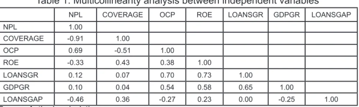
In order to eliminate multicollinearity between independent variables, a correlation analysis is presented in Table 1. The results in Table 1 indicate the highest collinearity of -0.91 between NPL and COVERAGE variables.
Table 1. Multicollinearity analysis between independent variables
NPL COVERAGE OCP ROE LOANSGR GDPGR LOANSGAP
NPL 1.00 COVERAGE -0.91 1.00 OCP 0.69 -0.51 1.00 ROE -0.33 0.43 0.38 1.00 LOANSGR 0.12 0.07 0.70 0.73 1.00 GDPGR 0.10 0.04 0.54 0.58 0.65 1.00 LOANSGAP -0.46 0.36 -0.27 0.23 0.00 -0.25 1.00
Source: Author’s calculations
In order to avoid multicollinearity between NPL and COVERAGE and over-parameterization
by including too many independent variables as well as to check the robustness of the
coefficients, the following four regressions will be estimated:
4 The market capitalization to GDP as a measure of size and stock turnover to GDP as a measure of liquidity of the Macedonian Stock Exchange is relatively low at an average of 7.16% and 1.43%, respectively, for the period from 1996 by 2012 (see World Development Indicators).
5 For the variables BUFFER, NPL, COVERAGE and ROE, the available quarterly data cover the period 2004Q4 to 2013Q3 and for the variable OCP quarterly data are available from 2006Q1 to 2013Q3. Concerning the previous periods, the data are annual for these variables. Therefore, in order to cover these data gaps and econometric results to be valid by encompassing a period of at least 10 years, the annual data for the above variables before 2004Q4 and 2006Q1 have been interpolated in a simple manner i.e. the annual value is allocated to the appropriate quarters.
The choice of the appropriate methodology for estimating these regressions depends on the integrative features of each individual variable (stationary or non stationary variables) as well as on their endogenous nature. Therefore, the Johansen cointegration technique (Vector Error Correction Model) will be applied as the most appropriate in order to estimate the regressions 7, 8, 9 and 10. The Johansen technique allows variables to be taken with
the same order of integration and uses lags in order to mitigate the problem that might
arise from the endogenous variables (Haris and Sollis, 2003). Additionally, this technique provides long-run equilibrium coefficients and the error correction mechanism (ECM) which presents the speed of adjustment of short-run disequilibrium towards long-run equilibrium. It should be noted that all studies presented in the literature review given above use panel econometric techniques. The data for the Macedonian banks are mostly available at the level of the total banking sector for the given period from 2003Q2 to 2013Q3 (individual banks data are not available for this period) and therefore the VECM technique is the most
appropriate econometric technique to be used in this study, rather than panel econometric
technique.
Estimation of the econometric model and results
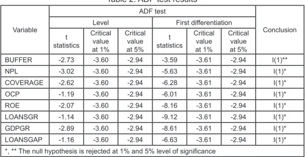
Before applying the Johansen co-integration technique, each variable included in the empirical model has to be tested for its order of integration i.e. checking whether the variables are stationary or non-stationary. Therefore, two tests were used: Augmented Dickey Fuller (ADF) and Phillips Perron (PP). The results of the unit root tests are presented in the table 2.
Table 2. ADF test results
Variable
ADF test
Conclusion Level First differentiation
t statistics Critical value at 1% Critical value at 5% t statistics Critical value at 1% Critical value at 5% BUFFER -2.73 -3.60 -2.94 -3.59 -3.61 -2.94 I(1)** NPL -3.02 -3.60 -2.94 -5.63 -3.61 -2.94 I(1)* COVERAGE -2.62 -3.60 -2.94 -6.28 -3.61 -2.94 I(1)* OCP -1.19 -3.60 -2.94 -6.01 -3.61 -2.94 I(1)* ROE -2.07 -3.60 -2.94 -8.16 -3.61 -2.94 I(1)* LOANSGR -1.14 -3.60 -2.94 -9.12 -3.61 -2.94 I(1)* GDPGR -2.89 -3.60 -2.94 -8.61 -3.61 -2.94 I(1)* LOANSGAP -1.16 -3.60 -2.94 -6.63 -3.61 -2.94 I(1)* *, ** The null hypothesis is rejected at 1% and 5% level of significance
Source: Author’s calculations
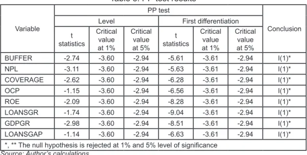
The results of both tests for stationarity indicate that the variables are non-stationary in the levels and they become stationary after the first differentiation, or are integrated of first order I(1). Furthermore, the Johansen co-integration procedure proceeds with determining the order of Vector Auto Regression (VAR) and identification of how many lags need to be included in the regression in order to mitigate the endogenous problem. For the order of VAR, information criteria such as: Likelihood Ratio (LR), Final Prediction Error (FPE), Akaike
(AIC), Schwarc (SC) and Hannan-Quinn (HQ) will be considered and the choice depends on the compliance of the majority of these criteria regarding the appropriate lag. Additionally, a review of the residual diagnostic tests (serial correlation, normality and homoscedasticity) will be carried out in order to check the validity of the chosen VAR based on the information criteria. The results of the information criteria and diagnostic tests for the regressions from 7 to 10 are presented in tables 4 to 11.
Table 3. PP test results
Variable
PP test
Conclusion Level First differentiation
t statistics Critical value at 1% Critical value at 5% t statistics Critical value at 1% Critical value at 5% BUFFER -2.74 -3.60 -2.94 -5.61 -3.61 -2.94 I(1)* NPL -3.11 -3.60 -2.94 -5.63 -3.61 -2.94 I(1)* COVERAGE -2.62 -3.60 -2.94 -6.28 -3.61 -2.94 I(1)* OCP -1.15 -3.60 -2.94 -6.56 -3.61 -2.94 I(1)* ROE -2.09 -3.60 -2.94 -8.28 -3.61 -2.94 I(1)* LOANSGR -1.74 -3.60 -2.94 -9.04 -3.61 -2.94 I(1)* GDPGR -2.98 -3.60 -2.94 -8.51 -3.61 -2.94 I(1)* LOANSGAP -1.14 -3.60 -2.94 -6.63 -3.61 -2.94 I(1)* *, ** The null hypothesis is rejected at 1% and 5% level of significance
Source: Author’s calculations
Table 4. VAR lag order selection criteria’s for the regression 7
BUFFER = f(NPL, OCP, ROE, LOANSGR, GDPGR)
Lag LR FPE AIC SC HQ
0 NA 35754.1800 27.5116 27.7676 27.6034
1 223.8570 212.4196 22.3622 24.15377* 23.00502* 2 52.70275* 202.9552* 22.18136* 25.5085 23.3751
3 26.5587 499.9117 22.6996 27.5623 24.4443
* indicates the order of VAR according to each criterion Source: Author’s calculations
Table 5. Diagnostic tests for the regression 7
Diagnostic tests for VAR = 2 in the regression 7; BUFFER = f(NPL, OCP, ROE, LOANSGR, GDPGR) Calculated
statistics Critical value at 1% Conclusion
H0: No serial correlation in the residuals 38.47 58.62
H0: Normality in the residuals 40.33 26.22 *
H0: Homoscedastic residuals 491.01 576.49
* indicates rejection of the null hypothesis at 1% level of significance Source: Author’s calculations
Table 6. VAR lag order selection criteria’s for the regression 8
BUFFER = f(NPL, OCP, ROE, LOANSGAP)
Lag LR FPE AIC SC HQ
0 NA 16043.3700 23.8724 24.0857 23.9489
1 248.9590 30.9739 17.6102 18.88988* 18.06935* 2 39.41547* 29.18832* 17.48457* 19.8306 18.3263
3 23.7509 44.7559 17.7340 21.1464 18.9583
* indicates the order of VAR according to each criterion Source: Author’s calculations
Table 7. Diagnostic tests for the regression 8
Diagnostic tests for VAR = 2 in the regression 8; BUFFER = f(NPL, OCP, ROE, LOANSGAP) Calculated
statistics Critical value at 1% Conclusion
H0: No serial correlation in the residuals 26.49 44.31
H0: Normality in the residuals 27.88 23.21 *
H0: Homoscedastic residuals 316.30 359.91
* indicates rejection of the null hypothesis at 1% level of significance Source: Author’s calculations
Table 8. VAR lag order selection criteria’s for the regression 9
BUFFER = f(COVERAGE, OCP, ROE, LOANSGR, GDPGR)
Lag LR FPE AIC SC HQ
0 NA 766081.1000 30.5762 30.8322 30.6681
1 222.9097 4688.1230 25.4565 27.24799* 26.09925* 2 56.03838* 3939.919* 25.14729* 28.4744 26.3410 3 31.2442 7677.7980 25.4312 30.2940 27.1759 * indicates the order of VAR according to each criterion
Source: Author’s calculations
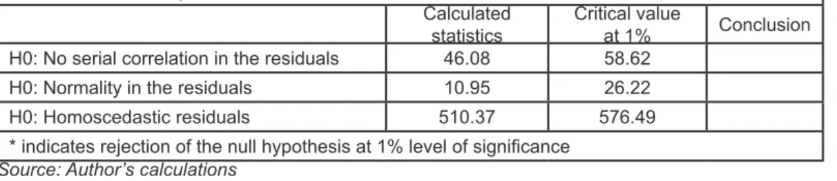
Table 9. Diagnostic tests for the regression 9
Diagnostic tests for VAR = 2 in the regression 9; BUFFER = f(COVERAGE, OCP, ROE, LOANSGR, GDPGR)
Calculated
statistics Critical value at 1% Conclusion
H0: No serial correlation in the residuals 46.08 58.62 H0: Normality in the residuals 10.95 26.22 H0: Homoscedastic residuals 510.37 576.49 * indicates rejection of the null hypothesis at 1% level of significance
Table 10. VAR lag order selection criteria’s for the regression 10
BUFFER = f(COVERAGE, OCP, ROE, LOANSGAP)
Lag LR FPE AIC SC HQ
0 NA 511876.1000 27.3352 27.5484 24.4117
1 250.4034 945.9259 21.0292 22.30890* 21.48837* 2 40.74217* 850.1430* 20.8562 23.2023 21.6980 3 30.9371 953.7629 20.79317* 24.2056 22.0175 * indicates the order of VAR according to each criterion
Source: Author’s calculations
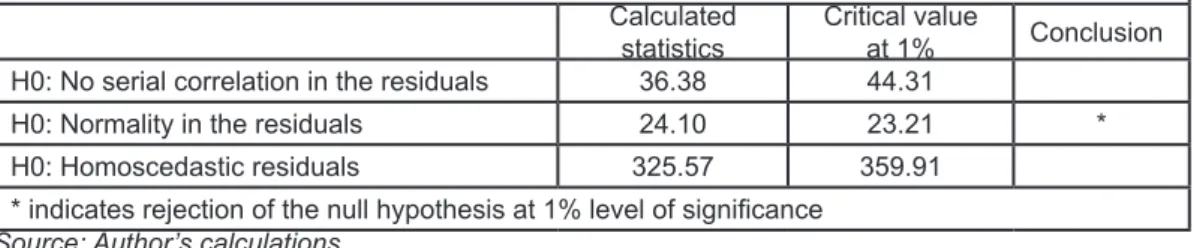
Table 11. Diagnostic tests for the regression 10
Diagnostic tests for VAR = 2 in the regression 10; BUFFER = f(COVERAGE, OCP, ROE, LOANSGAP)
Calculated
statistics Critical value at 1% Conclusion
H0: No serial correlation in the residuals 36.38 44.31
H0: Normality in the residuals 24.10 23.21 * H0: Homoscedastic residuals 325.57 359.91
* indicates rejection of the null hypothesis at 1% level of significance Source: Author’s calculations
As can be seen from Tables 4, 6, 8 and 10, the majority of information criteria suggest the involvement of two lags or value of VAR = 2 within the regressions7, 8, 9 and 10 and in addition the results of the diagnostic tests suggest appropriate specificity of all four regression equations under the order of VAR = 2 despite the rejection of the normal distribution hypothesis in the tables 5, 7 and 11.The rejection of the normality hypothesis can render invalid t and F tests of the coefficients for all four regressions. Nevertheless, according to Gujarati (2003), the non fulfillment of the assumption of the normal distribution of the residuals, does not necessarily mean misspecification of the regressions given the fulfillment of the homoscedasticity hypothesis and the size of the sample under investigation. Since homoscedasticity hypothesis is not rejected in any of the specifications presented in the tables 5, 7, 9 and 11, and the sample in this paper for the period 2003Q2 to 2013Q3 is the longest available sample for the Macedonian banking sector, it can be considered that t and F tests asymptotically follow normal distribution and therefore the regressions are correctly specified.
The next step in the Johansen integration analysis is to test for the presence of the co-integration vectors among the variables in the regressions 7, 8, 9 and 10. Two test statistics are available for this purpose; the first one is based on the trace of the stochastic matrix and the second one on the maximum Eigen value of the stochastic matrix. In this study, only the trace of the stochastic matrix test will be considered because of its’ advantage that can be drawn when the residuals are not normally distributed (Harris and Sollis, 2003).
Table 12. Co-integration rank test: trace statistics for the regressions 7, 8, 9 and 10
Regression 7 Regression 8 Regression 9 Regression 10
Trace stat Critical value at 1% Trace stat Critical value at 1% Trace stat Critical value at 1% Trace stat Critical value at 5% Null hypothesis: no
co-integration 129.35 127.71 80.28 77.82 127.45 127.16 73.99 69.82
Alternative hypothesis: at
most 1 co-integration vector 93.47 97.6 47.54 54.68 93.18 97.12 46.44 47.86
Source: Author’s calculations
According to the trace of the stochastic matrix test there is one co-integration vector at 1 percent level of significance for the regressions 7 to 9 and 5 per cent level of significance for the regression 10.Obtaining one cointegration vector implies that the vector can be normalized upon the dependent variable i.e. BUFFER. When normalized with respect to BUFFER, it is obtained the following co-integration vector.
Table 13. Normalized co-integrating vectors and estimated long run coefficients for the regressions 7, 8, 9 and 10
Regression 7 Regression 8 Regression 9 Regression 10
NPL 0.70 * 0.80 * Standard errors (0.1) (0.17) COVERAGE 0.16 ** 0.17 Standard errors (0.06) (0.2) OCP 0.06 ** 0.05 0.29 * 0.35 * Standard errors (0.03) (0.04) (0.04) (0.09) ROE 0.19 * 0.21 ** -0.13 0.14 Standard errors (0.06) (0.1) (0.08) (0.31) LOANSGR -0.37 * -1.05 * Standard errors (0.1) (0.2) GDPGR -0.09 -0.17 Standard errors (0.07) (0.14) LOANSGAP -0.06 -0.59 Standard errors (0.09) (0.38) Speed of adjustment (ЕCМ) 0.08 0.18 ** -0.12 0.03 Standard errors (0.16) (0.08) (0.08) (0.02)
* and ** indicate that the null hypothesis is rejected at 1% and 5% level of signifficance
Source: Author’s calculations
The results for the estimated coefficients regarding the regressions 7, 8, 9 and 10, shown in the table 13 indicate that the capital buffer of the Macedonian banking sector is generally determined by its exposure to risks and the profitability and not from the economic cycle. The results indicate that variables for the ex-post exposure to credit risk (NPL and COVERAGE) have a positive influence on BUFFER. The average effect of increasing NPL by one percentage point is 0.7 and 0.8 percentage points in the regressions 7 and 8 respectively,
under the condition that other factors remain unchanged, while COVERAGE coefficient is statistically significant only in the regression 9 and has an average effect of 0.16 percentage points. In compliance with the theory explained above, the coefficient before COVERAGE variable is with lower magnitude than the coefficient before NPL. LOANGR as ex-ante measure of credit risk is with a negative coefficient and it is -0.37 in the regression 7and -1.05 in the regression 9. OCP manifested statistically significant positive effect on BUFFER by 0.06; 0.29 and 0.35 percentage points in the regressions 7, 9 and 10, and its effect is not statistically significant in the regression 8.
ROE, as expected, manifested a positive and statistically significant impact in the regression 7 and 8. Regressions 7 and 8 imply an influence of ROE of 0.19 and 0.21 percentage point on the BUFFER, under ceteris paribus.
The coefficients for the economic cycle variables GDPGR and LOANSGAP suggest a negative and statistically insignificant impact on BUFFER in all regressions. This result is probably due to the fact that lending in Macedonian economy as a transition economy
has not yet reached its equilibrium level, and probably another reason would be that the
Macedonian GDP has not suffered from significant endogenous shocks would affect the banking sector significantly to increase the capital at the expense of limited credit.
The coefficient in front of the Error Correction Mechanism (ECM) measures the speed of adjustment of the BUFFER to its equilibrium level. The negative sign of this coefficient will allow the dependent variable to reach its’ equilibrium level. Namely, if the dependent variable is above the long-term equilibrium, then the negative value of this coefficient allows that it be reduced and equilibrium be reached. ECM coefficient in the regressions 7, 9 and 10 is positive, but statistically insignificant. The statistical insignificance of this coefficient probably indicates that the capital buffer of the Macedonian banking sector is in the initial equilibrium. This result is likely due to the high level of capitalization of the banks in Macedonia. The ECM coefficient is positive and statistically significant at the 5% level only in the regression 8 and implies that the disequilibrium of the BUFFER expands.
Conclusion and recommendations for the policy makers
The estimated coefficients before ex-post (NPL and COVERAGE) and ex-ante measures (LOANSGR) of the credit risk exposure of the Macedonian banks indicate that banks have
no tendency to create capital much earlier during the lending, but afterwards, when the
credit risk materializes. The econometric results also indicate that banks increase their
capital buffer when market risk increases, while the economic cycle has not statistically
significant effect.
It can be concluded from the results that banks in Macedonia are shortsighted, viewed from the perspective that they do not respond to ex-ante credit risk. As mentioned above, according to Tabak et al. (2011), banks that do not allocate capital in terms of credit
growth are myopic because they do not allocate capital anticipatively to protect against
unexpected losses from the materialized credit risk in the future. However, the good thing is that Macedonian banks reinvest their earnings as indicated by ROE variable and partially mitigate this problem of shortsightedness.
From that perspective, the recommendations of this study indicate that NBRM is required
to prepare research and econometric models to determine the equilibrium level of loans in
the Macedonian economy as implied by the Basel III Accord. By monitoring the equilibrium level of loans, NBRM can act proactively by prescribing a macro-prudential rule which would
impose an obligation on the banks to increase their capital whenever loans deviate upward
of their equilibrium level. In this way, the stability of the Macedonian banking sector will be further strengthened. Additional recommendation based on the findings of this paper is taking additional measures to stimulate the development of the Macedonian Stock Exchange. With a developed stock exchange, banks will have easier access to alternative sources of capital, besides their reinvested profits.
To overcome the shortcomings of this study, we give a recommendation to other researchers who would work on this issue. This research in the future could be improved by using panel techniques. Also, it would be good to include variable for the size of the banks and the deposits in the economy, in order to determine whether banks follow moral hazard. The big banks that fulfill the criteria too big to fail usually are predisposed to maintain less capital, because they believe that if getting into financial problems, they will be bailed out by the state. The impact of deposits on capital buffer should also be explored in terms of moral hazard. Namely, in terms of insured deposits, banks exhibit risky behavior and might not increase the capital because of the existence of the deposit insurance fund to cover the cost of depositors if banks are faced with eventual problems.
References
Atici, G. and Gursoy, G., (2013) The Determinants of Capital Buffer in the Turkish Banking System, International Business Research, Vol. 6. No. 1.
Ayuso, J., Perez, D. and Saurina, J, (2002) Are Capital Buffers Pro-Cyclical? Evidence from Spanish Panel Data ,Banco de Espana, Research Working Paper 0224.
Boucinha, M. (2008) The Determinants of Portuguese Banks’ Capital Buffers, Banco de Portugal, Working Paper.
D’Avack, F. and Levasseur, S. (2007) The Determinants of Capital Buffers in CEECs,
Observatoire Francais des Conjonctures Economiques, No. 28.
De Bondt, G. J. and Prast H. M. (1999) Bank Capital Ratios in the 1990: Cross-Country Evidence Central Bank of the Netherlands, Banca Nazionale del Lavoro Quarterly Review
212, 71–97.
Gersl, A. and Seidler, J. (2012) Credit Growth and Countercyclical Capital Buffers: Empirical Evidence from Central and Eastern European Countries, Charles University Prague, Faculty of Social Sciences, Institute of Economic Studies, Working Papers IES.
Gujarati, D. (2003) Basic Econometrics. Fourth Edition. New York, McGraw Hil.
Harris, R. and Sollis, R. (2003) Applied Time Series Modelling and Forecasting, Chichester,
Jokipii, T. and Milne, A. (2006) The cyclical behaviour of European bank capital buffers,
Bank of Finland, Research Paper 17.
Kleff, V. and Weber, М. (2005) How Do Banks determine Capital? Evidence From Germany,
ZEW Discussion Paper 03/66, University of Mannheim.
Lindquist, K. (2003) Banks’ Buffer Capital: How Important is Risk, Norges Bank. Working Paper(KGL) 12.3.03 Preliminary.
Stolz, S. and Wedow, M. (2011) Banks Regulatory Capital Buffer and the Business Cycle: Evidence for Germany, Deutsche Bundesbank, Discussion Paper, No.07/2005.
Tabak, B. M., Noronha, A. C. and Cajueiro, D. (2011) Bank Capital Buffers, Lending Growth and Economic Cycle: Empirical Evidence for Brazil, Bank for International Settlements,