Munich Personal RePEc Archive
The Gender Pay Gap: Micro Sources and
Macro Consequences
Morchio, Iacopo and Moser, Christian
University of Vienna, Columbia University
11 May 2018
Online at
https://mpra.ub.uni-muenchen.de/99549/
The Gender Pay Gap:
Micro Sources and Macro Consequences
∗Iacopo Morchio† Christian Moser‡ April 9, 2020
Abstract
We use administrative linked employer-employee data from Brazil to document that a large share of the gender pay gap is explained by women working at relatively low-paying employers. To shed light on the gender pay gap across employers, we establish three novel facts on revealed-preference ranks of employers by gender. First, employment is concentrated among high-ranked but not necessarily high-paying employers for both genders. Second, women’s ranking of employ-ers is less increasing in pay compared to that of men. Third, both pay and ranks of a given employer differ between women and men. To rationalize these facts, we develop an empirical equilibrium search model featuring endogenous gender differences in pay, amenities, and recruiting intensities across employers. The estimated model suggests that compensating differentials explain one-fifth of the gender gap, that there are significant output and welfare gains from eliminating gender differences, and that an equal-pay policy fails to close the gender pay gap.
Keywords: Worker and Firm Heterogeneity, Misallocation, Compensating Differentials, Discrimination,
Em-pirical Equilibrium Search Model, Linked Employer-Employee Data
JEL Classification:E24, E25, J16, J31
∗We thank Daron Acemoglu, Jim Albrecht, Jorge Alvarez, Roc Armenter, Jesper Bagger, Erling Barth, Martin Beraja, Mary Ann Bronson, Sydnee Caldwell, Rebecca Diamond, Rafael Dix-Carneiro, David Dorn, Niklas Engbom, Mikhail Golosov, Émilien Gouin-Bonenfant, Kyle Herkenhoff, Jonas Hjort, Philipp Kircher, Francis Kramarz, Kory Kroft, David Lagakos, Tzuo Hann Law, Rasmus Lentz, Ben Lester, Ilse Lindenlaub, Paolo Martellini, Guido Menzio, Magne Mogstad, Ben Moll, Giuseppe Moscarini, Andreas Mueller, Makoto Nakajima, Tommaso Porzio, Pascual Restrepo, Isaac Sorkin, Kjetil Storeslet-ten, Coen Teulings, Gabriel Ulyssea, Gianluca Violante, Susan Vroman, and Pierre Yared for valuable comments and discus-sions. We also thank attendants at the 2018 GEA Conference, the 2019 AEA Annual Meeting, the 2019 Search and Matching Network Conference, the 2019 Bank of Italy/CEPR/IZA Conference, the 2019 SED Annual Meeting, the 2019 NBER Sum-mer Institute, the 2019 Stanford SITE Workshop, the 3rd Dale T. Mortensen Centre Conference, the Boston Macro Juniors Conference, the 2020 Columbia Junior Micro Macro Labor Conference, and seminar participants at Columbia University, Boston University, CREST, Iowa State University, the University of Oslo, the University of Bristol, the University of Ed-inburgh, the University of Vienna, the Johannes Kepler University Linz, the Federal Reserve Bank of Philadelphia, and Temple University for helpful comments. Ian Ho and Rachel Williams provided outstanding research assistance. Moser gratefully acknowledges financial support from the Ewing Marion Kauffman Foundation and the Sanford C. Bernstein & Co. Center for Leadership and Ethics at Columbia Business School. Any errors are our own.
†Department of Economics, University of Vienna. Email:[email protected]. ‡Graduate School of Business, Columbia University. Email:[email protected].
1
Introduction
During the past decades, the introduction of gender in economic theory and measurement has had a profound impact on studies of labor markets and the macroeconomy. A common thread in these stud-ies is the robust empirical finding of a gender pay gap that is partly explained by gender imbalances in employment across different types of jobs. The implications of this finding crucially depend on whether the observed pay and employment of women relative to men reflects gender-specific prefer-ences over jobs or barriers in the labor market. The goal of this paper is to identify the microeconomic sources of the gender pay gap and to assess its macroeconomic consequences.
Our contribution is threefold. First, we use linked employer-employee data to establish novel facts on employment segregation, pay heterogeneity, and revealed-preference ranks across employers by gender. Second, we rationalize these facts by developing and estimating a new empirical equilibrium search model featuring endogenous gender differences in pay, amenities, and recruiting intensities across employers. Third, we use the estimated model to decompose the empirical gender pay gap, to quantify the output and welfare gains from moving to an economy with no gender differences, and to evaluate the effects of a counterfactual equal-pay policy. In doing so, we provide the first estimates of output and welfare losses from firm-level gender misallocation.
We base our empirical analysis on rich linked employer-employee data from Brazil between 2007 and 2014. The presence of a large gender earnings gap of around 14 log points makes it interesting in its own right to study the sources of gender inequality in a nation of over 200 million people. Such a study is made possible by Brazil’s remarkable data infrastructure, which contains detailed information on gender-relevant labor market variables, including workers’ educational attainment, occupation, contractual work hours, and employment histories with information on parental leaves.
We document significant employer segregation, with large differences in female employment shares across employers, even within sectors. To understand the link between employer segregation and the gender pay gap, we estimate an empirical specification with gender-specific employer pay components developed byCard et al.(2016) who, in turn, build on the seminal two-way fixed effects (FEs) framework byAbowd, Kramarz, and Margolis(1999, henceforth AKM). Controlling for worker heterogeneity, we find a gender pay gap of around 8 log points accounted for by gender-specific em-ployer pay heterogeneity, with women sorting to lower-paying emem-ployers relative to men.
To assess the extent to which the gender pay gap across employers reflects gender-specific tastes versus obstacles, we construct revealed-preference rankings of employers using PageRanks (Page et
al., 1998; Sorkin,2018) estimated separately by gender. The PageRank is a network centrality mea-sure that quantifies the attractiveness of an employer based on the network of worker flows between employers. Intuitively, higher-ranked employers poach many workers from other high-ranked em-ployers and lose few workers to low-ranked emem-ployers. Importantly, these PageRanks are estimated independently of any information on employer sizes or pay.
Based on estimated employer pay and revealed-preference ranks, we establish three novel facts. First, employment is concentrated among high-ranked but not necessarily high-paying employers for both genders. That is, employers’ revealed-preference ranks are different from pay ranks for both women and men. Second, revealed-preference employer ranks are increasing in pay for both genders, but more so for men than for women. In other words, women are relatively more attracted to employ-ers with low pay but high values of nonpay characteristics. Third, both within and across gendemploy-ers, there is significant heterogeneity in employers’ revealed-preference ranks conditional on pay. Specif-ically, both pay and the rank of a given employer differ between women and men.
To rationalize these facts, we develop a new empirical equilibrium search model featuring en-dogenous gender differences in pay, amenities, and recruiting intensities across employers. The model remains analytically tractable while accommodating several competing explanations for the gender pay gap, including employer productivity differences (Burdett and Mortensen,1998), gender-specific compensating differentials (Rosen, 1986), statistical discrimination (Arrow, 1971) based on expected employment transitions, and taste-based discrimination (Becker, 1971). The model gives rise to gender-specific job ladders with notable properties. The equilibrium wage equation is log-additively separable in a worker component and a gender-specific employer component, providing a microfoundation for the specification used in Card et al.(2016) and our own empirical investiga-tion. Endogenous worker transitions may be associated with wage declines. Low-productivity and discriminatory employers survive in equilibrium. Finally, equilibrium spillovers of discrimination imply that even employers without regard for gender offer different pay to men compared to women. A key challenge is to separately identify the competing explanations for the gender pay gap. We identify four sets of gender-specific model parameters using information on worker flows and em-ployer pay across genders. We estimate, emem-ployer-by-emem-ployer, gender-specific amenity values as residuals between employers’ relative pay and revealed-preference ranks in a set of bilateral com-parisons. We use empirical worker flows to obtain estimates of labor market parameters by gender, which give rise to heterogeneity in statistical discrimination by firms based on expected employment transitions. The conditional equilibrium pay gap between coworkers of different genders within
em-ployers identifies firm-level parameters guiding emem-ployers’ preferences over genders. Finally, we nonparametrically estimate each employer’s gender-specific hiring costs from their empirical recruit-ing intensities among nonemployed workers.
The estimated model is qualitatively and quantitatively consistent with our empirical facts. Fur-thermore, the estimation results shed light on the (unobserved) microstructure of labor markets for men and women. Employer pay, ranks, and amenities are positively correlated within employers across genders. Employer ranks are relatively more increasing in pay for men, but more increasing in amenity values for women. We find compensating differentials for both genders. Employers’ prefer-ence for men over women increases with employer productivity, consistent withBecker(1971)’s idea that discrimination cannot survive among low-productivity firms with close-to-zero economic profits. Our firm-level identification allows us to link structural estimates of employer heterogeneity to observed employer characteristics in the data. We find that women put relatively higher value on hours flexibility and parental leave benefits, while men are relatively less averse to pay fluctuations and health risks. Empirical proxies for more-wofriendly employers include higher routine man-ual and nonroutine cognitive-interpersonal task intensities, higher female employment shares and employing women in top-paid positions, and greater financial accountability. These estimates speak to different reasons why some employers are not gender-blind, including taste-based discrimination
(Becker,1971) and gender-specific comparative advantages (Goldin,1992).
With the estimated equilibrium model in hand, we simulate a number of counterfactuals that shed light on the sources and consequences of the gender pay gap. In a nonlinear structural decomposition, we find that compensating differentials in the form of gender-specific amenities explain 1.3 log points (18 percent) of the gap, employer tastes explain 5.4 log points (73 percent), and gender-specific hiring costs account for 5.6 log points (76 percent) of the gap. However, given the estimated distribution of pay and nonpay characteristics across employers, closing the gender pay gap may or may not be welfare-improving. We find that moving to an economy without gender differences is associated with output gains of 3.5 percent and welfare gains of 3.3 percent, reflecting firm-level misallocation of talent
(Hsieh et al.,2019). In contrast, a hypothetical equal-pay policy is mostly output- and welfare-neutral,
though it has redistributive effects.
Related literature. Several macroeconomic studies have focused on the drivers of trends in female
labor force participation, including structural change (Ngai and Petrongolo,2017;Buera et al.,2019), culture (Fernández et al.,2004; Fernández and Fogli,2009), technology (Greenwood et al.,2005;
Al-banesi and Olivetti, 2016), and information (Fogli and Veldkamp, 2011; Fernández, 2013). Related work has linked changes in female participation to economic growth (Heathcote et al.,2017;Hsieh
et al.,2019), unemployment (Albanesi and ¸Sahin,2018), business cycles (Fukui et al.,2019;Albanesi,
2020), and declining dynamism (Peters and Walsh,2019). Whereas previous macroeconomic studies have focused on data at the national, geographic, sectoral, or occupational level, our work highlights firm-level drivers of women’s employment and pay in relation to aggregate output and welfare.
The firm is a natural unit of analysis for studying productivity and factor input distortions in relation to macroeconomic outcomes (Restuccia and Rogerson,2008;Hsieh and Klenow,2009;Lentz
and Mortensen,2008;Bagger et al.,2014). Little prior work has connected firms’ gender composition
to aggregate output and welfare. If gender-specific barriers impede women’s relocation to higher-productivity firms, the gender pay gap may be associated with efficiency losses from misallocation of talent (Hsieh et al.,2019). By combining a rich equilibrium model with detailed linked employer-employee data, we provide the first estimates of output losses from firm-level gender misallocation. At the same time, our findings emphasize that output losses do not necessarily reflect welfare losses. A burgeoning literature highlights firm heterogeneity in explaining empirical pay dispersion for otherwise identical workers based on AKM’s seminal contribution (Card et al.,2013;Goldschmidt and
Schmieder,2017;Alvarez et al.,2018;Card et al.,2018;Gerard et al.,2018;Song et al.,2018). We build
onCard et al.(2016)’s empirical specification with gender-specific employer pay components. By
es-timating this specification on Portuguese data, they decompose the gender pay gap across employers into sorting and rent sharing terms. The fundamental sources of the gender pay gap, in particular the sorting and rent sharing terms, remain less understood. By providing a microfoundation for this specification based on worker and firm optimization, our equilibrium model can rationalize gender-specific sorting and rent-sharing patterns, and hence the empirical gender pay gap.
Our empirical equilibrium search model builds on the pioneering framework of Burdett and
Mortensen(1998).Bontemps et al.(1999,2000) estimate variants of this framework with heterogeneity
in firm productivity. Other important extensions and empirical applications includePostel-Vinay and
Robin(2002),Cahuc et al.(2006),Moscarini and Postel-Vinay(2013),Meghir et al.(2015),Engbom and
Moser(2018), andBagger and Lentz(2018). In all these models, firms are ex ante heterogeneous in
only one dimension, namely productivity. As a consequence, all workers agree on a common ranking of firms based purely on pay considerations. To rationalize our empirical facts on heterogeneity in employer pay and ranks by gender, we develop and estimate a tractable model with multiple dimen-sions of firm heterogeneity: productivity, amenity costs, hiring costs, and preferences over genders.
Other models have addressed gender issues in the labor market. For example, Black (1995),
Bowlus (1997), Bowlus and Eckstein (2002), Albanesi and Olivetti (2009), Flabbi (2010), Gayle and
Golan (2011), and Amano-Patiño et al. (2019) study different forms of wage discrimination. It is
well known that discrimination is hard to empirically distinguish from unobserved productivity dif-ferences or compensating differentials. In our framework, linked employer-employee data with in-formation on worker transitions and coworker wages is necessary to separately identify employer preferences over gender from other dimensions of job heterogeneity.
Gender-specific compensating differentials à la Rosen (1986) have been empirically studied by
Goldin and Katz(2011,2016).Goldin(2014) andErosa et al.(2019) highlight the gender-specific value
of job flexibility, which is underlined by recent experimental evidence (Mas and Pallais,2017,2019;
Wiswall and Zafar,2017). Theoretical models withnonspecificjob amenities have been developed by
Hwang et al.(1998),Lang and Majumdar(2004), andAlbrecht et al. (2018). Sullivan and To(2014),
Hall and Mueller (2018), and Luo and Mongey (2019) estimate nonspecific amenity values using
survey data. These studies are silent on specific job characteristics underlying nonspecific amenity values. Others have estimated the values of specific job amenities like employer health insurance
(Dey and Flinn, 2005), job security (Jarosch,2015), occupational fatality risk (Lavetti and Schmutte,
2018), commuting costs (Le Barbanchon et al.,2019;Flemming,2020), regional preferences (Heise and
Porzio,2019), and working conditions (Bonhomme and Jolivet,2009;Maestas et al.,2018). These
stud-ies do not relate the value of specific amenitstud-ies to the overall value of job amenitstud-ies. We bridge these two strands of the literature by first estimating nonspecific amenity values and then relating them back to specific employer characteristics. Like Taber and Vejlin(2016) andXiao(2020), we estimate nonspecific amenity values using linked employer-employee data. Unlike them, we identify gender-specific parameters employer-by-employer without relying on distributional assumptions or indirect inference. Sorkin(2018) and Lamadon et al.(2019) also estimate nonspecific firm-level amenity val-ues from linked employer-employee data. Our focus, in contrast to theirs, is on gender.Sorkin(2017) combines PageRanks with a partial-equilibrium framework to study gender differences in pay and amenities, highlighting gender differences in the exogenous offer distribution. As a complement to this prior work, our equilibrium model provides a theory of endogenous gender differences in offer distributions, which we leverage to study the effects of a counterfactual equal-pay policy.
Outline. The rest of the paper is structured as follows. Section 2 introduces the data. Section 3
the identification strategy. Section 6 presents estimation results. Section 7 conducts model-based counterfactuals. Finally, Section8concludes.
2
Data
2.1 Dataset and Variables
Dataset. Our main data source is theRelação Anual de Informações Sociais(RAIS) linked
employer-employee register administered by the Brazilian Ministry of Labor and Employment. Survey response by all tax-registered firms is mandatory and misreporting is deterred through threat of audits and fines. The data are available from 1985 onward, with coverage becoming near universal in 1994. Since 2007, the data contain detailed information on reasons and lengths of worker absences, including parental leaves. In 2015, the country entered a severe recession associated with a large drop in aggre-gate economic activity. Therefore, we focus on the eight-year period from 2007 to 2014. This leaves us with a large dataset of over 538 million employment records.
Variables. The data contain unique identifiers for workers and establishments.1 Although reports
are annual, we observe for each job spell the precise start and end dates, mean monthly earnings (henceforth “earnings”), and contractual work hours (henceforth “hours”). This allows us to avoid aggregation bias in classifying job-to-job transitions (Moscarini and Postel-Vinay,2018). Our baseline analysis uses earnings with flexible indicator controls for hours. However, for parts of our analysis we also construct hourly wages (henceforth “wages”) as earnings divided by the number of hours. Other key variables include gender in two categories, race in five categories, nationality in 37 cate-gories, educational attainment in nine catecate-gories, worker age in years, five-digit sector codes with 672 categories, municipality codes with 5,565 categories, six-digit occupation codes with 2,383 categories, and tenure in years. In addition, the data contain start and end dates of any absences from work and the reason for absence. We exploit the full panel dimensions of the data going back to 1985 with the tenure variable to impute actual (not just potential) formal-sector work experience in years.2
1All of our analysis is at the level of the establishment, which we intercheangably refer to as “employer” or “firm.” 2The distinction between actual and potential experience is important in general but explains little of the empirical
2.2 Sample Selection
We first restrict attention to male and female workers between the ages of 18 and 54 who worked at least one hour per week with earnings at or above the federal minimum wage. We then keep for each worker-year combination the highest-paid among all longest employment spells. Next, we iteratively drop singleton observations defined either by the combination of establishment identifier and gender or by worker identifier. We also impose a minimum establishment size threshold of ten nonsingleton workers per year on average.3 Finally, we require that establishments appear in our sample in at least four out of the eight years. Together, the last two selection criteria ensure that we are dealing with a set of reasonably large and stable establishments for which pay policies and amenity values can be credibly estimated.
To separately identify worker and employer pay components, we followAbowd et al. (2002) in constructing the largest connected set, where connections are formed through worker mobility be-tween establishments over time. In the language of graph theory, there are two types of connected sets. Aweakly connected setis one in which each establishment is connected to another establishment through at least one incoming or outgoing worker. Astrongly connected setis one in which each estab-lishment is connected to another node through at least one incoming and one outgoing worker. For the AKM model to be identified, it is sufficient to restrict attention to weakly connected sets. However, to estimate revealed-preference ranks of employers using PageRanks requires restricting attention to strongly connected sets (Sorkin, 2018). Therefore, we restrict attention to the largest strongly con-nected set (henceforth “concon-nected set”).
2.3 Summary Statistics
Table 11in Appendix A.2presents summary statistics on observations in the connected set in 2007, in 2014, and pooled across 2007–2014.4 In the pooled sample, we have over 231 million worker-years, corresponding to over 55 million unique workers and over 222,000 unique establishments. Around 38 percent of these observations are for women. The raw gender gap in earnings is around 14 log points and the gap in wages is around 6 log points. Compared to women, men are more likely to be nonwhite and hold at most a middle school degree.5 Men are significantly younger, work at smaller
3Following Sorkin(2018), nonsingleton workers are those who are observed at least one more time at a future date.
While the RAIS data cover only Brazil’s formal sector, the employer size restriction implies that the vast majority of informal establishments would be excluded from our analysis in any case (Ulyssea,2018;Dix-Carneiro et al.,2019).
4Also in AppendixA.2, we show the same summary statistics in the data before making sample selections and restricting
the data to the connected set (Table12) and comparing the two samples (Table13).
and younger establishments, work more hours, and have less tenure compared to women.6
3
Employer Heterogeneity and the Gender Gap
A classical Mincerian analysis of the gender gap in pay is presented in AppendixB.1. Standard Min-cerian controls only partly explain the empirical gender gap. Thus, building on AKM’s seminal con-tribution, we investigate the role of employer heterogeneity in relation to the gender gap.
3.1 Gender Segregation Across Employers
Women made up 38 percent of Brazil’s formal sector employment over the period of 2007–2014. How-ever, women were highly segregated across employers, even within industries. Figure 1 shows a histogram of female employment shares in 2014. Around 28 percent of establishments had less than 10 percent women among their workforce. In contrast, if women were equally distributed across employers, we would see a single bar of height 10 in the 30–40 percent category.
Figure 1. Histogram of female employment shares, 2014
0 1 2 3 4 5 6 7 8 9 10 Density 0.0 0.1 0.2 0.3 0.4 0.5 0.6 0.7 0.8 0.9 1.0 Female employment share
Overall
Source:Authors’ calculations based on RAIS.
We show in AppendixB.2 that gender segregation is a robust empirical phenomenon over time (Figure12), within sectors (Figure13), and across different employer sizes (Figure14). Figure15 in AppendixB.3shows that employment levels of men and women within establishments are positively but imperfectly correlated. In Appendix B.4, we quantify the degree of gender segregation across employers by defining and estimating an employer segregation index, which we find to be higher than analogous indices estimated across industries, occupations, or states.
3.2 Quantifying Employer Pay Heterogeneity
To understand the link between employer segregation and the gender pay gap, we estimate a wage equation with gender-specific employer pay components developed byCard et al.(2016), building on the seminal two-way FEs specification by AKM. This allows for the possibility that a given employer has two pay policies—one for each gender. Formally, we model earnings of individual i in yeart working at establishmentj= J(i,t), denotedyijt, as
yijt= Xitβ+αi+1[genderi = M]ψMj +1[genderi =F]ψFj +εijt, (1)
whereXitis a vector of gender-specific worker characteristics including a set of restricted
education-age dummies as well as dummies for hours, occupation, tenure, actual experience, and education-year combinations;αi is a person FE;ψjM andψFj are the male and female employer FEs, respectively; and
εijtis a residual term.7By including a set of person FEs, this specification controls for selection of men
and women across establishments based on unobserved time-invariant worker characteristics such as ability. In estimating equation (1), our main focus is on estimates of the gender-specific employer FEs,
ψM
j andψFj.
As is the case in all two-way fixed models, at least one normalization must be made regarding the intercept or mean of the employer FEs versus the person FEs. In our case, the model with gender-specific employer FEs requires two normalizations—one for each gender. Consistent with the the-oretical model presented later, we followCard et al. (2016) and Gerard et al.(2018) in normalizing the employer FEs of both genders to be of mean zero in the restaurant and fast-food sector, which, arguably, is populated by low-surplus employers.8
We now turn to our main object of interest in equation (1), namely the gender-specific employer FEs.9 Panel (a) of Figure 2 plots the distribution of employer FEs by gender. The distribution for women has visibly lower mean and lower variance than that for men. Panel(b)of the figure shows the distribution of within-employer differences in FEs for dual-gender establishments. The distribution is relatively dispersed compared to its mean of around 2 log points.
7To identify age, time, and worker FEs simultaneously, we restrict the age-pay profile to be flat around ages 45–49, which
is approximately consistent with empirical raw-earnings profiles. See AppendixB.5for details.
8For robustness, we experimented with alternative normalizations for gender-specific employer FEs. Separately, we
have repeated our analysis based on a wage equation without worker FEs, making the normalization redundant.
9In AppendixB.5, we present auxiliary results relating to the AKM equation, including estimated gender-specific hours
FEs (Figure16), occupation FEs (Figure17), actual-experience FEs (Figure18), tenure FEs (Figure19), education-year FEs (Figure20), and education-age FEs (Figure21).
Figure 2. Predicted AKM employer FEs for women and men (a) Gender-specific employer FE distributions
0.0 0.5 1.0 1.5 2.0 2.5 3.0 3.5 Density −1.0 −0.8 −0.6 −0.4 −0.2 0.0 0.2 0.4 0.6 0.8 1.0
Gender−specific AKM employer FE
Men Women
(b) Gender-specific employer FE distributions
0 1 2 3 4 5 6 7 8 Density −0.5 −0.4 −0.3 −0.2 −0.1 0.0 0.1 0.2 0.3 0.4 0.5
AKM employer FE gap (male − female)
Source:Authors’ calculations based on RAIS.Note:Dashed vertical line shows mean of the distribution.
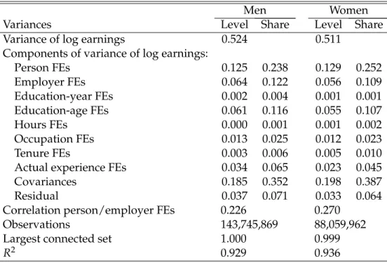
Table1shows a log-earnings variance decomposition.10 Men have a slightly higher variance of log earnings, with 52.4 log points, compared to 51.1 log points for women. For both genders, the largest variance component is due to estimated worker FEs, which account for 24 percent for men and 25 percent for women. Employer FEs account for 12 percent of the variance of earnings for men and 11 percent for women. The positive covariance terms are primarily attributed to the covariance between worker and employer FEs, education-age and employer FEs, and actual experience and employer FEs. The correlation between person and employer FEs is around 23 percent for men and 27 percent for women. For each gender, the largest connected set spans close to the full data. Finally, the model explains around 93 percent of the variation in log earnings.
10To be precise, Table1presents plug-in estimators of the variance components. In ongoing work, we are adapting
the leave-one-out estimator byKline et al.(2019), which implements a jackknife bias correction for limited-mobility bias (Andrews et al.,2008,2012), to a dataset of significantly larger size like ours.
Table 1. Variance decomposition based on gender-specific employer FEs model
Men Women
Variances Level Share Level Share Variance of log earnings 0.524 0.511
Components of variance of log earnings:
Person FEs 0.125 0.238 0.129 0.252 Employer FEs 0.064 0.122 0.056 0.109 Education-year FEs 0.002 0.004 0.001 0.001 Education-age FEs 0.061 0.116 0.055 0.107 Hours FEs 0.000 0.001 0.001 0.002 Occupation FEs 0.013 0.025 0.012 0.023 Tenure FEs 0.003 0.006 0.005 0.010 Actual experience FEs 0.034 0.065 0.023 0.045 Covariances 0.185 0.352 0.198 0.387 Residual 0.037 0.071 0.033 0.064 Correlation person/employer FEs 0.226 0.270
Observations 143,745,869 88,059,962 Largest connected set 1.000 0.999
R2 0.929 0.936
Source:Authors’ calculations based on RAIS.Note:Variance components based on earnings equation (1).
3.3 Between Versus Within-Employer Pay Differences
From here on we will focus on differences in the gender-specific employer components (henceforth “gender gap”). Using a Oaxaca-Blinder decomposition, we can write the gender gap as
γe ≡Ei,thψM J(i,t) genderi= M i −Ei,thψF J(i,t) genderi=F i =Ei,thψM J(i,t)−ψFJ(i,t) genderi= M i | {z }
within-employer gender pay gap
+Ei,thψF J(i,t) genderi= M i −Ei,thψF J(i,t) genderi=F i | {z }
between-employer gender pay gap
(2) =Ei,t h ψMJ(i,t)−ψFJ(i,t)genderi=F i | {z }
within-employer gender pay gap
+Ei,t h ψMJ(i,t)genderi= M i −Ei,t h ψJM(i,t)genderi=F i | {z }
between-employer gender pay gap
. (3)
Equations (2) and (3) are two alternative decompositions of the total gender gap,γe, into two terms.
Thewithin-employer pay gaporpay-policy componentis the mean difference in gender-specific employer FEs weighted by the distribution of men and women, respectively. It reflects differences in pay be-tween women and men at the same establishment. Thebetween-employer pay gaporsorting component is the difference between genders in mean male-employer FEs and female-employer FEs, respectively. It reflects differences in pay between men and women due to their different allocations across
estab-lishments.11
Figure22in AppendixB.6graphically illustrates estimates of the two components of the decom-positions in equations (2) and (3). Results of the decomposition are shown in Table2. Out of the total gender pay gap of 8.4 log points, 24 percent (5 percent) is attributed to the pay-policy component in Decomposition 1 (2). The remainder is attributed to the sorting component. This evidence suggests that women systematically work at lower-paying employers compared to men.
Table 2. Oaxca-Blinder decompositions of the gender pay gap due to employer heterogeneity Pay-policy component Sorting component Gender pay gap Level Share Level Share Decomposition 1 0.084 0.020 0.241 0.064 0.759 Decomposition 2 0.084 0.004 0.047 0.080 0.953
Source:Authors’ calculations based on RAIS.Note:Decompositions 1 and 2 correspond to equations (2) and (3),
respectively.
3.4 Life-Cycle Patterns and Event Study Analysis Around Parental Leaves
An obvious candidate factor that may be behind some of the hitherto documented patterns is related to childbirth. In AppendixB.7, we study life-cycle patterns of employer pay by gender and parental status. In AppendixB.8, we conduct an event study analysis around childbirth, as proxied by parental leave, following the methodology inKleven et al.(2016). While we find significant gender gaps in par-ticipation and earnings associated with childbirth, our analysis suggests that firm pay heterogeneity isnotthe only, or even a very important, factor behind these gaps.
3.5 Revealed-Preference Employer Rankings by Gender
To what extent does the gender pay gap reflect a gender utility gap? To answer this question, one must take into account both pay and nonpay characteristics of jobs for both genders. To this end, we estimate gender-specific revealed-preference rankings of employers using the PageRank index. The PageRank is a network centrality measure developed by Page et al.(1998) to rank websites for the web search engine Google that was first used in an economic context bySorkin(2018).
In a labor market context, the PageRank is defined as follows. Let g ∈ {M,F}index a worker’s gender, let j ∈ Jg = {j
1,j2, . . . ,jNg} index a set of Ng gender-specific employers, and let t ∈ T
11Note that the sorting component is invariant to the choice of the normalization of gender-specific employer FEs.
Coin-cidentally, this will be the main object of interest in our study. The pay-policy component, on the other hand, depends on the normalization of men’s relative to women’s employer FEs.
index time. We denote byngj,j′,t the number of workers of gendergtransitioning from employerjto
employer j′ at timet, bynjg,j′ = ∑t∈T n g
j,j′,tthe time aggregation of gender-specific flows between the
two employers, and byngj,. = ∑j′ngj,j′the number of workers of gendergflowing out from employer
j. LetBg(j) = nj′ :ngj′,j ≥1 o
denote the set of employers who have ever lost a worker of gendergto employerj. Letd ∈[0, 1]be a damping factor. ThePageRank index,sg(j), is a probability distribution
over all employersj∈ Jgsuch that
sg(j) = 1−d Ng +d
∑
j′∈Bg(j) wgj′,jsg j′ , ∀j∈ Jg,∀g, (4) wherewgj′,j = n g j′,j/n gj′,. is a weight equal to the share of worker flows from employer j′ to employer
jas a fraction of all worker flows from employer j′. Intuitively, employers with a high PageRank index poach many workers from other employers with high PageRank indices and lose few workers to other employers with low PageRank indices. The damping factor drepresents the weight on the poaching term in a convex combination with equal employer weights. Based on PageRank indices, we compute gender-specificPageRanks rg(j)for every employerj ∈ Jg as the rank of the PageRank
indices, with the lowest rank normalized to 0 and the highest rank normalized to 100.
Interestingly, the PageRank index represents the asymptotic share of time a representative worker (“random surfer”) who switches jobs by following the network of empirical worker flows would spend at a given employer. FollowingSorkin(2018), we choose as the damping factord=1 in all our
applications. By estimating PageRank indices on the strongly connected set, we avoid absorbing states (“rank sinks”), in which a worker could get indefinitely stuck at an employer. This interpretation of the PageRank index is particularly close to the definition of an employer rank in a large class of on-the-job search models, including the one we develop. Note also that an employer’s PageRank does not directly depend on its pay or size. Indeed, in computing PageRanks, we did not use any information on worker wages or the number of workers at any employer.
Based on equation (4), we compute employer PageRanks separately by gender.12We now establish three facts relating to employer heterogeneity in pay and ranks within and across gender.13
12In AppendixB.9, we show that the resulting PageRanks are strongly but imperfectly correlated with gender-specific
employer FEs in pay. PageRank estimates are also strongly but imperfectly correlated with two other popular employer rank measures, namely the poaching rank (Moscarini and Postel-Vinay,2008;Bagger and Lentz,2018) and the net poach-ing rank (Haltiwanger et al.,2018;Moscarini and Postel-Vinay,2018). An advantage of the PageRank over the other two rank measures is that it uses more information per worker transition in constructing an employer ranking, which reduces spurrious misclassifications of employer ranks.
13For the remainder of this section, we will study gender-population-weighted estimates of the unweighted PageRanks
as described above. Note that PageRanks are not restricted to having any particular mean value (e.g., 50) by construction since the PageRank estimation is independent of the cross-sectional employment distribution.
Fact 1. Employment is concentrated among high-ranked but not necessarily high-paying employers for both genders.
Figure3compares the employment distributions of men and women across pay ranks and across employer ranks. Panel(a)shows employment is weakly positively related to pay for both genders. Panel(b), on the other hand, shows that employment is strongly related to employer ranks for both genders. Furthermore, the rank-based employment distribution of women looks relatively more sim-ilar to that of men than it does for the pay-based employment distribution. Women’s mean employer pay rank is 53.9 while men’s is 58.3, implying a gender gap in pay ranks of 4.4 percentiles. On the other hand, women’s mean employer rank is 73.7 while men’s is 74.4, implying a gender gap in em-ployer ranks of 0.7 percentiles.
Figure 3. Densities over pay ranks and employer ranks, by gender (a) Pay ranks
0.00 0.01 0.02 0.03 0.04 0.05 Density 0 10 20 30 40 50 60 70 80 90 100
Gender−specific pay rank
Male pay ranks Female pay ranks
(b) Employer ranks 0.00 0.01 0.02 0.03 0.04 0.05 Density 0 10 20 30 40 50 60 70 80 90 100
Gender−specific employer rank
Male employer ranks Female employer ranks
Source:Authors’ calculations based on RAIS.
Fact 2. Mean employer ranks are more increasing in pay ranks for men than for women.
Figure 4 shows that employer ranks are positively correlated with pay ranks for both men and women. However, the employer rank-pay gradient is steeper for men than for women, especially in the bottom half of employer pay rank distribution. This suggests that there exist low-paying jobs that are at the same time relatively attractive for women, and this is less so the case for men. Therefore, pay is a relatively more important determinant the overall evaluation of an employer for men than for women.14
14AppendixB.10presents several robustness checks. Figure27shows the relationship between employer ranks and pay
ranks across sectors. Table17shows that this fact is not driven by sectoral or geographic differences. Table18shows that this fact is consistent with the dynamics of pay for different worker transitions across employer ranks.
Figure 4. Employer rank and pay, by gender 0 10 20 30 40 50 60 70 80 90 100
Mean gender−specific employer rank
0 10 20 30 40 50 60 70 80 90 100
Gender−specific employer pay rank
Men Women
Source:Authors’ calculations based on RAIS.
Fact 3. There is significant heterogeneity in employer ranks conditional on pay within and across genders.
Figure5shows that there is significant dispersion in employer ranks conditional on pay for men in Panel(a)and for women in Panel(b). This suggests heterogeneity in employers’ nonpay character-istics.15 For both men and women, ranks are relatively more dispersed at low-pay employers than at high-pay employers. This suggests that establishments with high pay are also high in utility. This is consistent with either their pay being high enough to compensate for their level of (dis-)amenity, or alternatively, their amenities being high on top of their high pay.16
Figure 6shows that there is also significant within-employer between-gender dispersion in pay ranks in Panel(a)and in employer ranks in Panel(b). Pay and employer ranks are strongly positively correlated within employers across genders. This is consistent with the idea that an employer’s pro-ductivity and amenities, such as its location and certain benefit policies, are partly shared by its male and female workers. Cross-gender employer ranks are also relatively more dispersed than cross-gender pay ranks. This may reflect that productivity (e.g., technology or management practices) is shared more freely across genders compared to valuations of certain amenities (e.g., hours flexibility or parental leave policies). Finally, men and women closely agree on their rankings of top employers, both in terms of pay ranks and employer ranks, but agree less on lower-ranked employers.17
15Figure30in AppendixB.11shows that the standard deviation of employer ranks is similarly decreasing in employer
pay ranks for men and women.
16AppendixB.11shows that the same qualitative conclusions apply when, for robustness, we compare employer ranks
across pay ranks by industry for women (Figure28) and for men (Figure29).
17For robustness, AppendixB.11shows the same relation between female and male pay ranks (Figure31) and that
Figure 5. Percentiles of employer rank distribution conditional on pay ranks, by gender (a) Men 0 10 20 30 40 50 60 70 80 90 100
Percentiles of male employer ranks
0 10 20 30 40 50 60 70 80 90 100
Percentiles of male pay
P10 P25 P50 P75 P90 (b) Women 0 10 20 30 40 50 60 70 80 90 100
Percentiles of female employer ranks
0 10 20 30 40 50 60 70 80 90 100
Percentiles of female pay
P10 P25 P50 P75 P90
Source:Authors’ calculations based on RAIS.
Figure 6. Percentiles of female versus male employer pay and ranks (a) Pay 0 10 20 30 40 50 60 70 80 90 100
Percentiles of female pay
0 10 20 30 40 50 60 70 80 90 100
Percentiles of male pay
P10 P25 P50 P75 P90 (b) Ranks 0 10 20 30 40 50 60 70 80 90 100
Percentiles of female employer rank
0 10 20 30 40 50 60 70 80 90 100
Percentiles of male employer rank
P10 P25 P50 P75 P90
Source:Authors’ calculations based on RAIS.
4
Model
Addressing the empirical facts requires a structural model with the following ingredients. First and foremost, the model must allow for an employer’s revealed-preference rank to differ from its pay rank. To rationalize this, workers in the model value an employer’s amenities in addition to pay. Second, the model must generate differences in pay and amenities across employers. To rationalize this, the labor market is modeled as frictional. Third, the model must admit gender differences in pay, revealed-preference ranks, and employment within a firm. To rationalize this, employers in the model post gender-specific wages, amenities, and job vacancies. We combine these ingredients in an
equilibrium model of the labor market.
4.1 General Environment
A measure 1 of workers and measureEof firms meet in a continuous-time frictional labor market.
4.2 Workers
Workers are infinitely lived, risk neutral, and discount the future at rateρ. They permanently differ
in abilitya ∈ [a,a]and genderg ∈ {M,F}with measureµa,g such that∑g=M,F
´
aµa,gda = 1. At any
point in time, they find themselves either employed or nonemployed.18
Job search. While nonemployed, workers receive flow utilityba,gand engage in random job search
within segmented labor markets by worker type. Search is random in the sense that workers cannot direct their search to specific firms. Labor markets are segmented in the sense that workers search for jobs in a market specific to their type. While employed, workers receive flow utilityx =w+πequal
to the sum of their wage,w, and job amenity value, π. Employed workers also engage in on-the-job
search within the same segmented markets.
As a result of job search, workers receive regular job offers with arrival rate λua,g from
nonem-ployment and with rate λea,g from employment. While regular on-the-job offers admit free disposal,
workers also receive mandatory on-the-job offers (sometimes termed a “Godfather shock,” or an offer one cannot refuse) at rateλGa,g in both employment states. We think of the latter as capturing, among
other things, spousal relocation problems and other idiosyncratic reasons for switching jobs. We will write λe
a,g = sea,gλau,g andλGa,g = sGa,gλua,g, where sea,g and sGa,g are the relative hazards of regular and
mandatory on-the-job offers, respectively.
A job offer is an opportunity to work at some firm with associated wagewand amenity valueπ,
drawn from a distribution ˜F(w,π), which workers take as exogenous but that is determined endoge-nously through firms’ equilibrium decisions. Since a worker’s flow utilityx = w+πis sufficient for
summarizing their state, jobs will be ranked on a ladder according tox, and we can restrict attention to the implied flow-utility offer distributionF(x). A job can be terminated endogenously when a worker with flow utilityxin their current job accepts an offer from a higher-utility job at rateλea,g(1−F(x)),
18In mapping the model to the data, we think of the “nonemployed” in the model as capturing the pool of the
unem-ployed, workers on temporary (parental or other) leave, workers marginally attached to the labor force, and workers in informal employment. The estimation of labor market parameters will take into account that some workers might spend longer periods outside of formal employment due to these factors.
or exogenously: at rateλG
a,gthe worker relocates to a randomly drawn job, and at rateδa,gthe worker
becomes nonemployed.
Value functions. The value of an employed worker of type (a,g) in a job with flow utility x is
summarized as follows: ρSa,g(x) =x+λea,g ˆ x′≥x Sa,g(x′)−Sa,g(x) dFa,g(x′) +λGa,g ˆ x′ Sa,g(x′)−Sa,g(x) dFa,g(x′) +δa,gWa,g−Sa,g(x). (5)
Analogously, the value of a nonemployed worker of type(a,g)is summarized as follows:
ρWa,g=ba,g+ (λua,g+λGa,g)
ˆ
x′
maxSa,g(x′)−Wa,g, 0 dFa,g(x′). (6)
Policy function. Strict monotonicity of the value functionSa,g(x)implies that the optimal job
accep-tance strategy of a nonemployed worker will be characterized by a threshold rule with reservation flow utility φa,g. Thus, a nonemployed worker will accept an offer if x ≥ φa,g and reject it
other-wise. The reservation flow utility simply equals the sum of the flow value of nonemployment plus the forgone option value of receiving job offers while nonemployed:
φa,g =ba,g+ (λua,g−λea,g) ˆ x′≥φa,g 1−Fa,g(x′) ρ+δa,g+λaG,g+λea,g 1−Fa,g(x′)dx ′. (7)
Employed workers in a job with flow utilityxsimply accept any job that delivers flow utilityx′such thatx′ >x.
Nonemployment and utility dispersion. Since in equilibrium no firm will post a contract worth
less thanφa,gin any market(a,g), the steady-state nonemployment rate for each worker type is
ua,g=
δa,g
δa,g+λua,g+λGa,g
. (8)
The cross-sectional distribution of flow utilities is given by Ga,g(x) = Fa,g(x) 1+κe a,g 1 −Fa,g(x) ,
whereκe
a,g=λea,g/(δa,g+λGa,g)governs the effective speed of workers climbing the job ladder.
4.3 Firms
Firms differ in four dimensions. First, they have heterogeneous productivity p ∈ [p,p] ⊂ R++ as
in Burdett and Mortensen (1998). Second, firms differ in a set of employer wedges za,g ∈ [z,z] ⊂ R
representing the firm’s disutility from worker type(a,g), as inBecker(1971). Third, firms are hetero-geneous in a set of amenity cost shifterscπa,,0g > 0, as inHwang et al.(1998). Finally, firms differ in a
set of vacancy cost shifterscva,0,g > 0. Thus, a firm’s type is j = (p,{za,g}a,g,{cva,,0g}a,g,{caπ,,0g}a,g), which
we assume is distributed continuously according toΓ(j).
Wages, amenities, and job vacancies. Firms deliver value to workers through a combination of
two channels. First, they post in each market a wage rate wa,g that is constant for the duration of
the employment spell. Second, they also post a market-specific value of amenities πa,g. Following
Hwang et al.(1998), we assume that the cost of producing a level of amenitiesπa,gmust be paid per
worker of type(a,g)employed at the firm, and that the per-worker amenity flow cost can be written ascπ
a,g(πa,g) = cπa,,0g ×c˜πa,g(πa,g), where the function ˜caπ,g(·)satisfies ˜cπa,g(0) = 0, ∂c˜πa,g(0)/∂π = 0, and
∂c˜πa,g(π)/∂π,∂2c˜πa,g(π)/∂π2 > 0 for allπ > 0 and all(a,g). In order to recruit workers and produce
output, firms also postva,gjob vacancies in each market subject to flow costcva,g(va,g) =cva,0,g×c˜v(πa,g),
where the function ˜cv(·)satisfies ˜cv(0) = 0, ∂c˜v(0)/∂v = 0, and∂c˜v(v)/∂v,∂2c˜v(v)/∂v2 > 0 for all
v>0.
Production. A firm with productivity pemploying {la,g}a,g workers of each type produces output
according to the following linear production technology: y(p,{la,g}a,g) =p
∑
g=M,F
ˆ
a
ala,gda.
Employer wedges. In addition to output specified above, the model allows employers to care about
employing different worker types. We model this as a set of employer wedges {za,g}a,g which, as
two special cases, may capture either taste-based discrimination as inBecker(1971) or firm-level com-parative advantages in productivity across genders related to “brain versus brawn” (Goldin, 1992;
Rendall, 2018). We restrict these wedges to take the form za,g = 1[g = F]za, where za guides an
Value function. Firms post wages, amenities, and vacancies in each market to maximize
steady-state flow payoff. The valueΠ(j)of a firm of typej= (p,{za}a,{cav,,0g}a,g,{cπa,,0g}a,g)is given by
ρΠ(j) = max {wa,g,πa,g,va,g}a,g g=
∑
M,F ˆ a h pa−wa,g−cπa,g(πa,g)−za,g i la,g(wa,g,πa,g,va,g)−cva,g(va,g)da . (9) 4.4 MatchingThe effective mass of job searchers in market(a,g)equals Ua,g =µa,g
h
ua,g+sea,g(1−ua,g) +sGa,g
i
, ∀(a,g). (10)
The total mass of vacancies posted in market(a,g)across firm typesjequals Va,g =E
ˆ
j
va,g(j)dΓ(j), ∀(a,g). (11)
In the Diamond-Mortensen-Pissarides tradition, a Cobb-Douglas matching function with constant returns to scale combines the effective mass of job searchers with the total mass of job vacancies to produce a measure of matches between workers and firms,ma,g, according to
ma,g =χa,gVaα,gUa1,−gα, ∀(a,g),
where χa,g > 0 is the matching efficiency and α ∈ (0, 1) is the matching elasticity with respect to
aggregate vacancies. Define labor market tightness as
θa,g =
Va,g
Ua,g
, ∀(a,g). (12)
The job-finding rates among nonemployed workers,λua,g, the job-finding rates among the employed,
λea,g, the arrival rates of mandatory offers,λaG,g, and firms’ job-filling rates,qa,g, are given by
4.5 Firm Size Distribution
The following Kolmogorov forward (or Fokker-Planck) equation describes the law of motion of firm sizes given a firm’s flow-utility and vacancy policy (x,v), the market distribution of flow utilities Fa,g(x), and market tightnessθa,g:
˙ la,g(x,v) = h −δa,g−λea,g 1−Fa,g(x) −λGa,g i la,g(x,v) + " ua,g+ (1−ua,g)sae,gGa,g(x) +sGa,g ua,g+ (1−ua,g)sea,g+sGa,g # vqa,g.
Solving for the stationary firm size distribution, we find
la,g(x,v) = 1 δa,g+λGa,g+λea,g 1−Fa,g(x) 2 v Va,gµa,g (ua,g+saG,g)λua,g(δa,g+λGa,g+λea,g). (14) 4.6 Equilibrium Characterization
We define astationary equilibriumof the economy in AppendixC.1. The assumed market segmentation and linearity of the production technology allow us to keep this problem tractable in spite of the many dimensions of worker and firm heterogeneity. These assumptions allow us to divide the firm’s problem into separate subproblems by market. Conditional on productivity, a firm’s optimal choice in each market is essentially independent of all other markets, which means that we can solve the firm’s problem in each market in isolation.
For any posted wage-amenity combination, firms find themselves ranked on a market-specific lad-der according to their flow-utility offer x. An argument analogous to that inBurdett and Mortensen (1998) shows that the equilibrium offer distributionFa,g(x)and the cross-sectional distributionGa,g(x)
are continuous and strictly increasing forx >max n
pa−1[g=F]z, φa,g
o
in each market(a,g)up to some maximum value. Next, we characterize firms’ optimal policy functions.
Lemma 1(Optimal amenities). A firm’s optimal amenity policyπ∗a,g(·)is strictly decreasing in its amenity
cost shifter cπa,,0g and is invariant to all other parameters. Furthermore,0<cπa,g(π∗a,g)<π∗a,g.
Proof. See AppendixC.2.1.
Lemma1 extends to our setting a key result inHwang et al.(1998), who also assume that firms are heterogeneous in their convex-increasing per-worker cost of amenities. Inuitively, firms optimally offer amenities up to the point where the marginal cost of amenities equals that of wages, which equals one. That the cost-minimization problem does not depend on a firm’s productivity, employer
wedge, or recruiting costs follows from two assumptions: that worker utility is additively separable between wages and amenities and that the amenity cost is paid per worker. An implication of Lemma
1is that, due to the bijection between firm-specific amenity cost shifters and optimal amenity values, we can treat π∗a,g as an exogenous firm-level parameter. Furthermore, in model counterfactuals, a
firm’s optimal amenity choice remains at the estimated value unless there are changes to its amenity cost function relative to its wage cost function.
Define a firm’scomposite productivityin market(a,g)as ˜pa,g = pa+πa,g−cπa,g(πa,g)−za,g. We can
treat ˜pa,gas an exogenous firm characteristic, allowing us to rewrite the problem of a firm as
ρΠa,g(p˜a,g,cva,0,g) =maxx,v
n˜
pa,g−xla,g(x,v)−cva,g(v)
o
, ∀(a,g). (15)
Therefore, the current model is essentially isomorphic to one without amenities or employer wedges but with two modifications.19 First, productivity pis replaced by composite productivity ˜p. Second, wagesware replaced by flow utilityx. This isomorphism allows us to derive comparative statics with respect to the different components of ˜pa,g.
Lemma 2(Optimal market selection). A firm optimally employs workers in market(a,g)ifp˜a,g >φa,g.
Proof. See AppendixC.2.2.
A firm makes positive monetary profits if pa+πa,g−cπa,g(πa,g) > φa,g.20 However, Lemma 2
states that, due to the presence of employer wedges, this condition is neither necessary nor sufficient for a firm to select into a market. Depending onza in relation to the monetary surplus pa+πa,g−
cπa,g(πa,g)−φa,g in each market, the firm may hire any combination of genders: both, either one, or
none (in which case it does not operate).
Lemma 3(Optimal vacancies). A firm’s optimal vacancy policy v∗a,g(·)is strictly increasing in productivity
p, strictly decreasing in the vacancy cost shifter cva,0,g for all worker types, and strictly decreasing (constant) in
zafor women (men).
Proof. See AppendixC.2.3.
The intuition behind Lemma 3is that more productive firms have a higher marginal payoff per contacted worker; thus they invest more into recruiting both men and women. The opposite is true
19SeeEngbom and Moser(2018) for an example of such a model.
with regards to female vacancies at firms with a higher employer wedge in their payoff function. Naturally, firms with a higher vacancy cost post fewer vacancies for both genders.
Lemma 4(Optimal flow utility and wages). A firm’s optimal flow-utility policy x∗a,g(·) and wage policy
w∗a,g(·)are strictly increasing in p for all worker types, constant in the vacancy cost shifter cva,0,g for all worker
types, and strictly decreasing (constant) in the employer wedge zafor women (men).
Proof. See AppendixC.2.4.
Lemma 4 extends the comparative statics results with respect to wages in Mortensen (2003) to an environment with richer employment contracts (amenities and wages, instead of just wages) and richer sources of worker mobility (Godfather shocks and heterogeneous arrival rates from nonem-ployment and emnonem-ployment, instead of just homogeneous arrival rates). Intuitively, firms with a larger payoff from employing a given worker optimally offer workers higher utility through wages in order to attract and retain a larger workforce.
Lemma 5 (Optimal employment). A firm’s optimal employment l∗a,g(·) is strictly increasing in p for all
worker types, strictly decreasing in the vacancy cost shifter cva,0,g for all worker types, and strictly decreasing
(constant) in the employer wedge zafor women (men).
Proof. See AppendixC.2.5.
Lemma5states that firms with higher composite productivity ˜phave greater steady-state employ-ment, which is a combination of their rank in the job ladder, as guided by their flow-utility rank, and their recruitment intensity, as guided by the share of their aggregate-share of vacancies.
4.7 Equilibrium Wage Equation
The current equilibrium model provides a microfoundation for the decomposition of log wages into worker FEs and gender-firm FEs byCard et al.(2016), which is based on the seminal two-way FEs framework developed by AKM. To back up this claim, we provide a set of sufficient conditions for the log-wage decomposition to obtain as an equilibrium outcome in the model.
Assumption 1(Vacancy cost function). Vacancy-posting costs cva,,0gscale linearly in worker ability a:
Assumption 1 could reflect that recruiting costs be paid in terms of time given to new hires for orientation and training, or in terms of the time of equally skilled workers devoted to recruiting.
Assumption 2(Job offer arrival and separation rates). The relative arrival rates of optional job offers sEa,g,
that of mandatory job offers sGa,g, and separation ratesδa,gare constant in worker ability a:
sEa,g= sEg, sGa,g =sGg, δa,g=δg, ∀a
Assumption2allows for differential worker mobility across, but not within, genders.
Assumption 3(Amenity cost function). The amenity creation cost function cπa,g(π)takes on the following
piece-rate form: cπa,g(π) =acπg,0c˜ π a , ∀a
Assumption3states that the cost of creating amenities is proportional to worker ability, and that amenities are paid to worker as a piece rate in their ability. A natural interpretation for this would be that some amenities involve time spent off work, such as in the context of paid parental leave. In this case, the cost of providing some units of time in amenities to a worker scales linearly in the worker’s ability or forgone production due to the worker’s absence from the job.
Assumption 4(Flow values of nonemployment and employer wedges). The flow values of
nonemploy-ment ba,gand employer wedges zascale linearly in worker ability a:
ba,g =bga, za =za, ∀a
Assumption 4 ensures symmetry in participation and composite productivity across labor mar-kets. It may be justified by higher-ability workers also being more skilled at home production, and by employers being willing to give up a fraction of workers’ output to avoid interacting with them.
The following result links the structural model to the reduced-form approach in Section3.2.
Proposition 1(Equilibrium Wage Equation). Under Assumptions1–4, the equilibrium wage of a worker
with ability a and gender g at a firm with composite productivity p˜gand amenity cost shifter cπg,0is
lnwa,g ˜ pg,cπg,0 = |{z}αa “worker FE” + ψg ˜ pg,cπg,0 | {z } “gender-firm FE” , (16)
where αa=lna, ψg ˜ pg,cπg,0 =ln p˜g−π∗g cπg,0− ˜ pg ˆ ˜ p′≥φg 1+κe g h 1−Fg x∗g p˜gi 1+κe g h 1−Fg x∗ g(p˜′) i 2 dp˜′ . (17)
Proof. See AppendixC.2.6.
Proposition1shows that, under appropriate scaling assumptions, equilibrium wages in the model are log-additive between a worker component (“worker FE”) and a gender-specific firm component (“gender-specific firm FE”). The worker FEαais a strictly monotonic transformation of worker ability.
The gender-specific firm FEψg(p˜g,cπg,0)depends only on gender-firm–specific parameters, namely a
firm’s composite productivity ˜pg and its amenity cost shiftercπg,0. Therefore, the equilibrium model
provides a microfoundation for the wage equation with gender-specific employer pay components developed byCard et al. (2016) and used in our own empirical investigation. We will maintain As-sumptions1–4and focus on differences in gender-specific firm FEs between men and women for the remainder of the analysis.
4.8 Discussion of Equilibrium Properties
The above model has three notable equilibrium properties. First, the model can rationalize job-to-job transitions with wage declines. On one hand, workers receive exogenous relocation shocks that result in forced transitions from wagewtow′ < w. On the other hand, workers may endogenously
transition from wage-utility combination(w,x)to(w′,x′)withx′ > xbutw′ <w.
Second, “discriminatory” firms (as captured by the employer wedgez) can survive in a frictional environment.21 A prediction of Becker(1971)’s seminal framework of taste-based discrimination is that, in a competitive market, employers with a distaste for certain workers are driven out of the market. In contrast, in the current model, firms with nonzero employer wedges z survive in the presence of labor market frictions.
Third, even “nondiscriminatory” firms (as captured by z) may pay women less due tostatistical discriminationbased on gender-specific transition rates, due tocompensating differentials, or due to their
21We do not want to claim that the employer wedgezonly relates to discrimination. On the contrary, we think of it as
capturing many different mechanisms. Among such mechanisms, taste-based discrimination is of particular interest. All else being equal, higher taste-based discrimination against female workers is associated with higher values ofz.
equilibrium response to the presence of other discriminatory employers.
4.9 Discussion of Modeling Assumptions
We now turn to a brief discussion of some of the more restrictive modeling assumptions and their im-plications. A first set of assumptions made in the model is that output is linear within and additively separable across worker types. These assumptions allow for considerable analytical tractability, but we argue that they are also in line with our empirical evidence.
That output is linear within worker types is not particularly restrictive since a firm’s net payoff function is already concave due to the convex vacancy cost. Conceptually, there is no reason not to simultaneously allow for curvature in the ability-weighted number of workers of each type. However, if the marginal product of a given worker type were exceedingly high for small numbers of workers— as would be the case with standard constant-elasticity-of-substitution specifications—then we would see every firm employing a strictly positive mass of each worker type. This clearly would be at odds with the presence of single-gender firms in the data.
That output is additively separable across worker types ultimately allows the model to admit a log-linear wage equation, which is a requirement for us to be able to take the model to the data. Assuming complementarities between genders would lead to the counterfactual implication that no single-gender firms could exist. Supporting our assumption,Fukui et al.(2019) find a small crowd-out between women and men in the U.S. between 1970 and 2016. Therefore, it seems like a natural starting point to think of men and women as perfect substitutes in production.
A second assumption revolves around labor market segmentation by worker types, which allows firms to tailor wages, amenities, and vacancies to each market. This assumption considerably simpli-fies the analysis of the firm’s problem. We argue that the assumption is also reasonable and in line with salient empirical patterns.
Conceptually, that firms can direct wages and vacancies toward certain worker types may seem at odds with national nondiscrimination laws. But of course a firm need not publicly post a lower wage or invest less recruitment effort when hiring workers in order to discriminate. Such differences may naturally arise in more subtle ways when screening résumés, at the interview stage, and at the negotiation table (Goldin and Rouse,2000).
Empirically, there are also good reasons to adopt market segmentation. In particular, we have solved three “natural” modeling alternatives with clearly counterfactual predictions. A model with firms offering a single wage for workers of both genders would fail to account for the empirical
within-firm pay differences documented in Sections 3.2and3.3.22 A model in which amenities are shared across workers of both genders within a firm would counterfactually predict no dispersion in firm ranks conditional on gender-specific pay, which is at odds with Fact3from Section3.5. Models in which vacancy costs are over the sum of gender-specific vacancies or in which vacancies are not directed across genders fail to account for the empirical dispersion of female employment shares and hence the between-employer pay gap in the data.23
A third set of assumptions underlying Proposition1allow us to make significant progress in bring-ing the model to the data. One may expect that some of these assumptions do not hold exactly in the data. For example, when labor market parameters differ across ability levels, then the decomposition in equation (16) will not hold exactly. However,Engbom and Moser(2018) show that an AKM decom-position of log wage predicts around 99 percent of the variance of log earnings in data simulated from a model that allows for flexible variation in labor market parameters across ability types estimated to the same data from Brazil.
5
Identification Strategy
To bridge the model and the data, we connect key model objects with their empirical counterparts. Our starting point is the special case of the model characterized in Proposition1of Section4.7. Under the maintained assumptions, this allows us to pool workers of different ability types in the data and dropafrom all subscripts of this section. We adopt a three-step identification strategy.
5.1 Step 1: Employer Ranks
In the first step, we estimate revealed-preference ranks of employers by gender using the PageRank index (Page et al., 1998; Sorkin, 2018) described in Section 3.5. This constitutes a set of NM +NF
estimates, whereNMandNFare the numbers of establishments hiring men and women, respectively,
in the data. The PageRank index represents the asymptotic share of time a representative worker (“random surfer”) would spend at a given employer. This notion of employer rank coincides with that in the structural model of Section4, in which workers are less likely to endogenously separate
22We solve the model with gender-neutral wage offers later when simulating the effects of an equal-pay policy.
23We solve both of these models in AppendixC.3. The model with directed vacancy posting and a joint cost function
in AppendixC.3.1predicts that, with the exception of knife-edge cases, there exist no dual-gender firms. The model with undirected vacancy posting in AppendixC.3.2predicts that, quantitatively, there is far too little dispersion in female em-ployment shares compared to the empirical distribution we see in the data. We conclude that the benchmark model with targeted vacancies and separate cost functions is a good starting point for our investigation.
from, and more likely to accept offers at, higher-utility employers. In what follows, we conflate ranks and employer identities by indexing establishments by their rankrg ∈ {1, 2, . . . ,Rg}, where 1 is the
lowest andRgis the highest rank for workers of genderg.
5.2 Step 2: Labor Market Parameters
In the second step, we estimate labor market parameters by combining employer ranks from Step 1 with monthly information on worker flows.24 We seek gender-specific estimates of the cumulative density function (CDF) of offers Fgr, separation rates δg, job–finding rates from nonemployment λug,
the relative arrival rate of mandatory on-the-job offerssG
g, and rel