Examining the Use of Regression Models for Developing Crash Modification Factors

EXAMINING THE USE OF REGRESSION MODELS FOR DEVELOPING CRASH MODIFICATION FACTORS

A Dissertation by LINGTAO WU

Submitted to the Office of Graduate and Professional Studies of Texas A&M University

in partial fulfillment of the requirements for the degree of DOCTOR OF PHILOSOPHY

Chair of Committee, Dominique Lord Committee Members, Jeffrey Hart

Luca Quadrifoglio Yunlong Zhang Head of Department, Robin Autenrieth

May 2016

Major Subject: Civil Engineering

ii ABSTRACT

Crash modification factors (CMFs) can be used to capture the safety effects of countermeasures and play significant roles in traffic safety management. The before-after study has been one of the most popular methods for developing CMFs. However, several drawbacks have limited its use for estimating high-quality CMFs. As an

alternative, cross-sectional studies, specifically regression models, have been proposed and widely used for developing CMFs. However, the use of regression models for estimating CMFs has never been fully investigated. This study consequently sought to examine the conditions in which regression models could be used for such purpose.

CMFs for several variables and their dependence were assumed and used for generating random crash counts. CMFs were derived from regression models using the simulated data for various scenarios. The CMFs were then compared with the assumed true values. The findings of this study are summarized as follows: (1) The CMFs derived from regression models should be unbiased when the premise of cross-sectional studies were met (i.e., all segments were similar, proper functional forms, variables were independent, enough sample size, etc.). (2) Functional forms played important roles in developing reliable CMFs. When improper forms for some variables were used, the CMFs for these variables were biased, and the quality of CMFs for other variables could also be affected. Meanwhile, this might produce biased estimates for other parameters. In addition, variable correlation and distribution might potentially influence the CMFs and parameter estimates when improper functional forms were used. (3) Regression

iii

models did suffer from the omitted-variable bias. If some factors having minor safety effects were omitted, the accuracy of estimated CMFs might still be acceptable. However, if some factors already known to have significant effects on crash risk were omitted, the estimated CMFs were generally unreliable. (4) When the influence on safety of considered variables were not independent, the CMFs produced from the commonly used regression models were biased. The bias was significantly correlated with the degree of their dependence.

iv DEDICATION

v

ACKNOWLEDGEMENTS

First, I would like to express my deepest appreciation to my advisor,

Dr. Dominique Lord, for his constant guidance, encouragement and support throughout this dissertation. My committee members, Dr. Jeffrey Hart, Dr. Luca Quadrifoglio, and Dr. Yunlong Zhang, are greatly appreciated for their suggestions on this dissertation. Dr. Bruce X. Wang is also appreciated for his comments.

I also want to extend my gratitude to my colleagues in Texas A&M

Transportation Institute (TTI). Special thanks go to Mr. Robert Wunderlich, Dr. Troy Walden, Dr. David Bierling, Dr. Srinivas Geedipally, and Dr. Myunghoon Ko for their support on my research at TTI.

I would like to acknowledge International Road Federation and Research Institute of Highway, China for their financial support during my first year of Ph.D. study.

vi TABLE OF CONTENTS Page ABSTRACT ...ii DEDICATION ... iv ACKNOWLEDGEMENTS ... v TABLE OF CONTENTS ... vi

LIST OF FIGURES ... viii

LIST OF TABLES ... x

1. INTRODUCTION ... 1

2. BACKGROUND ... 7

2.1 Approaches for Estimating CMFs and Their Limitations ... 7

2.2 Nonlinear Relationships between Variables and Their Safety Effects ... 11

2.3 Safety Effects of Combined Treatments ... 14

2.4 Summary ... 17

3. METHODOLOGY ... 19

3.1 Simulation Analysis for Linear Relationships ... 19

3.2 Omitted Variable Problem ... 31

3.3 Nonlinear Relationships ... 32

3.4 Variable Correlation ... 36

3.5 Combined Safety Effect ... 38

3.6 Data Description ... 43

3.7 Summary ... 48

4. ESTIMATING THE QUALITY OF CMFS ... 49

4.1 Linear Relationships ... 49

4.2 Omitted Variables ... 56

4.3 Nonlinear Relationships ... 60

4.4 Variable Correlation ... 105

4.5 Combined Safety Effect ... 120

vii

5. VALIDATION USING OBSERVED DATA ... 130

5.1 Data Description ... 130

5.2 Estimated CMFs using Different Functional Forms ... 132

5.3 Volume-Only Model and “Full-Variable” Model ... 150

5.4 Summary ... 158

6. SUMMARY AND CONCLUSIONS ... 160

6.1 Summary of This Study... 161

6.2 Recommendations and Future Research Area ... 163

REFERENCES ... 166

viii

LIST OF FIGURES

Page

Figure 1 An Example Illustrating the Assumed CMF and CMF Derived from SPFs ... 26

Figure 2 Example Illustrating the Closest Line to a Curve ... 33

Figure 3 CM-Functions for Lane Width in Scenario IV (=0.5) ... 65

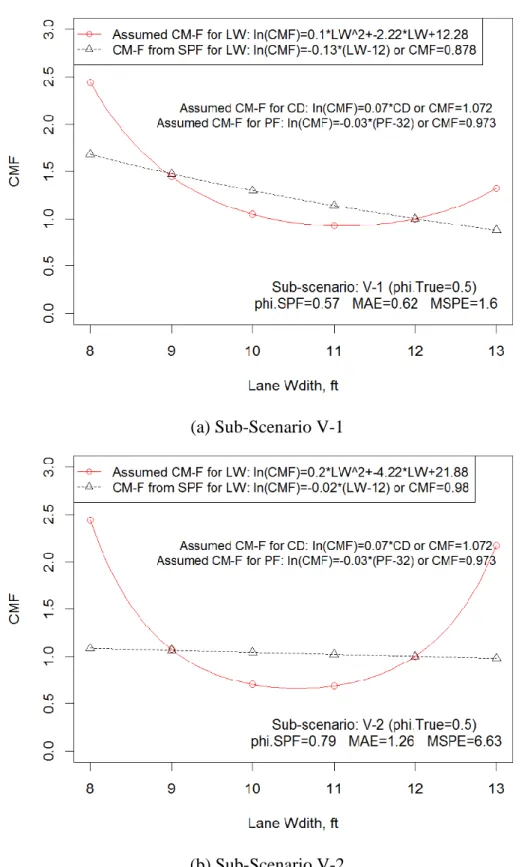
Figure 4 CM-Functions for Lane Width in Scenario V (=0.5) ... 74

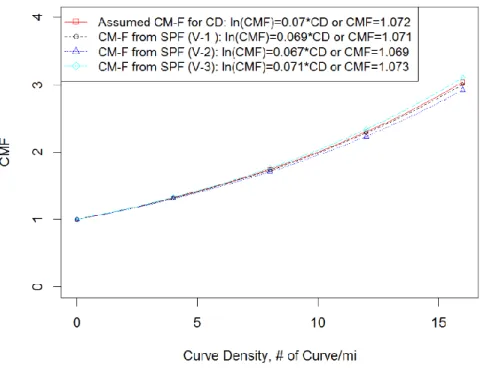
Figure 5 CM-Functions for Curve Density in Scenario V (=0.5) ... 79

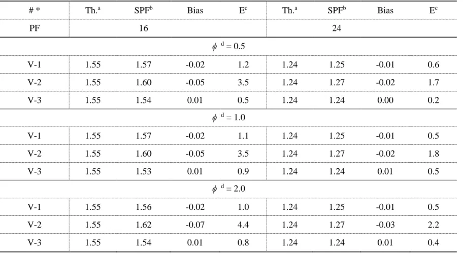
Figure 6 CM-Functions for Pavement Friction in Scenario V (=0.5) ... 79

Figure 7 CM-Functions for Lane Width in Scenario VI (=0.5) ... 91

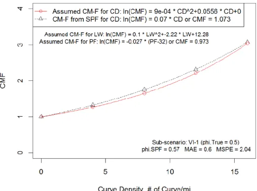
Figure 8 CM-Functions for Curve Density in Scenario VI (=0.5) ... 97

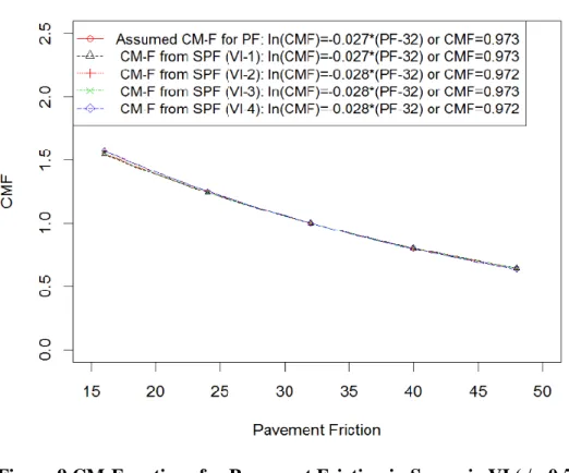
Figure 9 CM-Functions for Pavement Friction in Scenario VI (=0.5) ... 101

Figure 10 CM-Functions for Lane Width in Scenario VIII (=0.5) ... 112

Figure 11 Scatter Plots of Crash Counts and Lane Width ... 117

Figure 12 Example Illustrating the Effects of Variable Distribution on Regression ... 119

Figure 13 Error Percentage of CMFs for Lane Width in Scenario IX (=0.5) ... 125

Figure 14 Error Percentage of CMFs for Shoulder Width in Scenario IX (=0.5) ... 125

Figure 15 Scatter Plots of Crash Rate against Variables ... 132

Figure 16 Mean Crash Rate and Lane Width ... 134

Figure 17 CM-Function for Lane Width Derived using Observed Data (Linear)... 136

Figure 18 CM-Function for Lane Width Derived using Observed Data (Inverse) ... 138

Figure 19 CM-Function for Lane Width Derived using Observed Data (Exponential) . 140 Figure 20 CM-Function for Lane Width Derived using Observed Data (Log)... 142

ix

Figure 22 CM-Function for Lane Width Derived using Observed Data (Quadratic) .... 146

Figure 23 CM-Functions for Lane Width Derived using Observed Data (All) ... 148

Figure 24 Ninety-Five Percent Confidence Intervals ... 156

Figure 25 Mean AADT and Lane Width ... 157

x

LIST OF TABLES

Page

Table 1 Example of Simulated Crash Counts for N Segments ... 26

Table 2 Modeling Output of the Example Data ... 29

Table 3 Summary of Four Groups of Segments ... 40

Table 4 Summary of Sub-Scenarios in Scenario IX... 42

Table 5 Summary Statistics of Highway Segments for Scenarios I to VI ... 44

Table 6 MNL for Generating Lane Width (Baseline: 8 ft) ... 45

Table 7 Summary Statistics of Highway Segments for Scenarios VII and VIII ... 46

Table 8 Summary Statistics of Highway Segments for Scenario IX ... 47

Table 9 Results of Scenario I ... 51

Table 10 Results of Scenario II ... 55

Table 11 Results of Scenario III ... 57

Table 12 Assumed CM-Functions for Lane Width in Scenario IV ... 61

Table 13 Results of Scenario IV ... 63

Table 14 Bias and Error of CMFs for Lane Width in Scenario IV ... 67

Table 15 Assumed CM-Functions in Scenario V ... 71

Table 16 Results of Scenario V ... 73

Table 17 Bias and Error of CMFs for Lane Width in Scenario V ... 76

Table 18 Bias and Error of CMFs for Curve Density in Scenario V ... 80

Table 19 Bias and Error of CMFs for Pavement Friction in Scenario V ... 82

Table 20 Assumed CM-Functions for Curve Density in Scenario VI ... 87

Table 21 Assumed CM-Functions in Scenario VI ... 88

xi

Table 23 Bias and Error of CMFs for Lane Width in Scenario VI ... 93

Table 24 Bias and Error of CMFs for Curve Density in Scenario VI ... 99

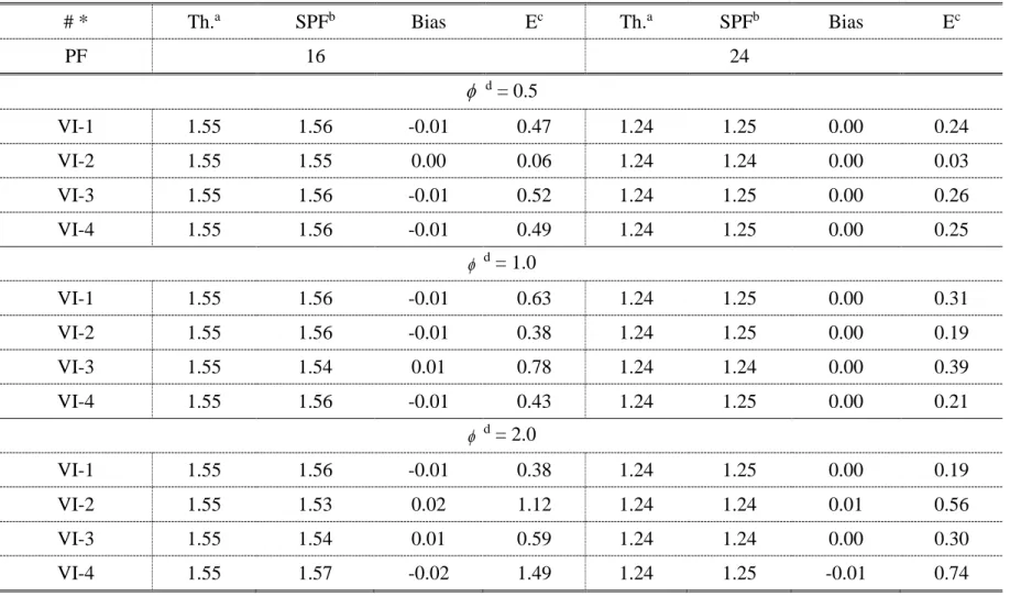
Table 25 Bias and Error of CMFs for Pavement Friction in Scenario VI ... 102

Table 26 Results of Scenario VII ... 107

Table 27 Results of Scenario VIII ... 111

Table 28 Bias and Error of CMFs for Lane Width in Scenario VIII ... 114

Table 29 Results of CMFs in Scenario IX ( = 0.5) ... 121

Table 30 Modeling Output of the an Experiment in Sub-Scenario IX-1 ... 128

Table 31 Summary Statistics of Observed Data ... 131

Table 32 Modeling Result of Observed Date with Linear Functional Form... 135

Table 33 Fitting Result of Inverse Functional Form for Lane Width ... 137

Table 34 Modeling Result of Observed Date with Inverse Functional Form ... 137

Table 35 Fitting Result of Exponential Functional Form for Lane Width ... 139

Table 36 Modeling Result of Observed Date with Exponential Functional Form ... 139

Table 37 Fitting Result of Log Functional Form for Lane Width ... 141

Table 38 Modeling Result of Observed Date with Log Functional Form ... 141

Table 39 Fitting Result of Power Functional Form for Lane Width ... 143

Table 40 Modeling Result of Observed Date with Power Functional Form ... 143

Table 41 Fitting Result of Quadratic Functional Form for Lane Width ... 145

Table 42 Modeling Result of Observed Date with Quadratic Functional Form ... 145

Table 43 Comparison of GOFs and Prediction Measurements ... 149

Table 44 “Bias” and “Error” of CMFs for Lane Width ... 151

Table 45 Modeling Result of Volume-Only Model ... 152

xii

Table 47 Results of CMFs in Scenario IX (= 1.0) ... 177 Table 48 Results of CMFs in Scenario IX ( = 2.0) ... 180

1

1. INTRODUCTION

A crash modification factor (CMF) is a multiplicative factor that can be used to reflect or capture changes in the expected number of crashes when a given

countermeasure or a modification in geometric and operational characteristics of a specific site is implemented (FHWA 2010; Gross et al. 2010; Wu et al. 2015). CMFs play a significant role in roadway safety management, including in safety effect evaluation, crash prediction, hotspot identification, countermeasure selection, and the evaluation of design exemptions. Several methods have been proposed for developing CMFs, such as the before-after (e.g., naïve or simple before-after, before-after with comparison group and empirical Bayes (EB) before-after), the cross-sectional (e.g., regression models and case-control), and expert panel studies among others (Gross et al. 2010). Amid these methods, before-after and cross-sectional studies are the most popular approaches (Shen and Gan 2003).

CMFs derived from before-after studies are based on the comparison of safety performance before and after the implementation of one or several treatments (or changes in the characteristics of the site(s)). Those derived from cross-sectional studies are based on the comparison in the safety performance of sites that have a specific feature with those that do not or are analyzed simultaneously based on datasets that contain a mixture of sites with different characteristics.

Over the last 15 years or so, the before-after study has been considered to be the best approach for developing CMFs (Gross and Donnell 2011; Gross et al. 2010). The

2

CMFs derived from before-after studies are usually believed to be more reliable than those produced from cross-sectional studies because it can directly account for changes that occurred at the sites investigated (Hauer 1997). However, although the before-after analysis is considered superior, high-quality CMFs derived from this approach is dependent on the availability of data (e.g., data availability for the before period, etc.) and the sample size (e.g., number of sites where the treatment of interest has been implemented, etc.). Furthermore, the estimated CMF can be biased if the

regression-to-the-mean (RTM) and site selection effects are not properly accounted for in the before-after study (Davis 2000; Hauer 1997; Lord and Kuo 2012). Lord and Kuo (2012) even noted that the EB method can still be plagued by significant biases if the data collected for the treatment and control groups do not share the exact same characteristics.

Given the limitations of before-after studies described above, researchers have proposed that cross-sectional studies could be used for developing CMFs (Bonneson and Pratt 2010; Noland 2003; Tarko et al. 1999). Although different types of cross-sectional studies have been proposed over the years, the regression model (also known as safety performance function or SPF) remains the method of choice for estimating CMFs, as reflected by the large number of CMFs documented in the Highway Safety Manual (HSM) (AASHTO 2010) and Federal Highway Administration (FHWA) CMF Clearinghouse (FHWA 2010) that are derived from regression models.

Even though regression models are popular for developing CMFs, some researchers have criticized their use for such purpose because they may not properly

3

capture the relationships between crashes and variables influencing safety (Hauer 2005b, 2010, 2014). There are several assumptions with using regression models. For example, the primary premise of a cross-sectional study is that all locations are similar to each other for all factors affecting crash risk except those of interest (Gross et al. 2010). However, this requirement can hardly be satisfied in practice. In addition, some other problems (e.g., sample size, omitted variables, functional forms, independence assumption, etc.) also influence the modeling result, and hence the quality of CMFs produced from the regression analyses. Under such conditions, the CMFs derived from regression models may potentially be biased. In this context, so far, nobody has

examined the statistical performance of CMFs that are developed using regression models. Thus, the primary objective of this study was to comprehensively investigate the robustness and accuracy of the CMFs derived from regression models. A secondary objective was to describe the conditions when the CMFs developed from regression models became unreliable and potentially biased. Note that, there has been some issues raised about whether or not cross-sectional studies are able to derive reliable cause-effect results, not only in traffic safety study, but also in other fields where this kind of

statistical method has been used, such as psychology, epidemiology, etc. (Hauer 2015). The objective of this study was not to prove that the cross-sectional analyses are able to reveal the cause and effect of traffic collisions. Rather, the aim was to raise the potential problems associated with the commonly used regression models (i.e., generalized linear models or GLMs) for developing CMFs.

4

To accomplish the objectives, the following four tasks were conducted in this study:

Task 1 – Validation of CMFs derived from regression models

This task evaluated the accuracy of CMFs derived from regression models considering the most common and simple form (i.e., the linear relationship) and assuming all the assumptions of cross-sectional studies were satisfied. The purpose of this task was to validate whether or not the CMFs produced from regression models were reliable under ideal conditions.

Task 2 – Omitted variables and the accuracy of CMFs

In task 1, all factors that influenced crash risk were assumed to be known. But this requirement can hardly be met in reality. In this task, some factors affecting crash risk were assumed to be unknown or unable to be captured by the models. The purpose of this task was to investigate how the omitted-variable problem influenced the CMFs derived from regression models. More specifically, it was to quantify the problem.

Task 3 – Nonlinear relationships and the accuracy of CMFs

In tasks 1 and 2, the variables were assumed to have linear relationships (in the logarithmic form) with crash risk. This was consistent with the commonly used GLMs. However, some studies indicated that this may not be the case. Some variables had been shown to have nonlinear and/or non-monotonic relationships with crash risk (Gross et al. 2009; Hauer 2004). Under such conditions, the commonly used GLM method might not be applicable, and the CMFs produced from these models could be biased, especially

5

around the boundary areas. The purpose of this task was to evaluate the CMFs derived from regression models when some variables had nonlinear relationships with crash risk.

Task 4 – Combined safety effects and the accuracy of CMFs

Factors influencing safety are always assumed to be independent of each other when modeling crashes using the common methods. However, this may not be realistic in practice (Gross et al. 2010). It is common that multiple treatments were implemented at a problematic entity (e.g., a hotspot) simultaneously, and these treatments might have overlap effects on reducing crashes especially when the target collision types were the same. The CMFs derived from regression models might be biased if the variables were actually not independent. The purpose of this task was to investigate how this

independence assumption influenced the accuracy of CMFs. This task is not about investigating the statistical correlation between variables, but the practical relationship and effects when multiple changes are applied simultaneously.

Each task contains one or multiple scenarios to assess the CMFs derived from regression models under various conditions.

This dissertation is divided into six chapters:

Chapter 2 documents the background about the commonly used approaches for developing CMFs, nonlinear relationships between variables and crash risk, and combined safety effects of multiple treatments.

Chapter 3 describes the methodologies used for estimating the quality of CMFs derived using regression models.

6

Chapter 5 validates the findings based on observed data.

And finally, Chapter 6 summarizes the key findings of this study and provides avenues for further research.

7

2. BACKGROUND

This chapter provides relevant background pertaining to CMFs in three aspects: (1) the commonly used CMF estimating methods; (2) nonlinear relationships between variables and crash risk; and (3) the combined safety effects of multiple treatments. 2.1 Approaches for Estimating CMFs and Their Limitations

This section briefly describes the commonly used methods that have been proposed for estimating CMFs. The description mainly focuses on their advantages and limitations.

As mentioned above, before-after and cross-sectional studies are the two main approaches used to estimate CMFs. The CMF for a countermeasure derived from a before-after study is estimated by the change in the number of crashes occurring in a period before the improvement and the number occurring after the improvement (Gross et al. 2010; Shen and Gan 2003). Four types of before-after studies have been proposed to estimate CMFs: naïve after, after with comparison group, EB before-after and full Bayes (FB) before-before-after studies. The naïve before-after study simply assumes the crash performance before improvement is a good estimate of what would be in the after period if the countermeasure had not been implemented (Hauer 1997; Shen and Gan 2003). This approach is considered to be less reliable, because it does not account for changes unrelated to the countermeasure. The before-after study with

8

comparison group and EB before-after methods were then proposed to overcome this issue. Gross et al. (2010) documented the details of these CMF developing methods.

Even though multiple before-after studies have been developed and widely used to estimate CMFs, the comparison results from before-after studies may be inaccurate if the following issues are not properly accounted for:

Sample size – There might be inadequate samples of sites where the countermeasures of interest have been implemented. This will lead to statistical uncertainty (Gross and Donnell 2011).

RTM effect – This bias is related to the level of correlation for sites that are evaluated during different time periods. Sites that have large (or very small) values in one time period (say before) are expected to regress towards the mean in the subsequent period (Hauer 1997; Hauer and Persaud 1983).

Site selection bias – This is related to the RTM, but its effects are different in that the sites are selected based on a known or unknown entry criteria (e.g., five crashes per year). These entry criteria lead to a truncated distribution, which influences the before-after estimate (Lord and Kuo 2012).

Mixed safety effects – This bias or issue is related to when more than two or more countermeasures are simultaneously implemented at a roadway site, and there can be changes in traffic volume, weather, etc. after the implementation of treatments. This makes it difficult to evaluate the safety effect of a single countermeasure (Gross and Donnell 2011; Gross et al. 2010).

9

In contrast to before-after studies, cross-sectional studies compare the safety performance of a site or group of sites with the treatment of interest to similar sites without the treatment in a single point in time (Gross et al. 2010). The cross-sectional studies for developing CMFs can be regrouped into three categories: regression, case control and cohort methods. The regression method is currently the most frequently used approach because of its simplicity. It is usually accomplished through multiple variable regression models or SPFs. The SPFs can be used to quantify the effect of a specific variable on the predicted crash occurrence and CMFs are then derived from the model coefficients (Gross et al. 2010; Tarko et al. 1999).

Many models have been proposed to predict safety performance and hence to develop CMFs or crash modification functions (CM-Functions) (Lord and Mannering 2010). Although recent studies have introduced some new models for transportation safety analysis (Chen and Persaud 2014; Mannering and Bhat 2014; Park et al. 2014a; Zou et al. 2013a), the GLM with a negative binomial (NB) error structure is still the most popular method for modeling traffic crashes. Despite the fact that regression models have been extensively used in traffic safety studies, there are still some limitations with this approach:

Similarity in crash risk – A primary premise of a cross-sectional study is that all locations are similar to each other in all other factors affecting crash risk (Gross et al. 2010). However, this assumption seems to be unattainable in practice.

Omitted variables – A variety of variables can influence crash risk, but not all of them are measurable or can be captured in practice for model inclusion. It is common

10

that some SPFs were developed with limited variables, for example, using the traffic volume as the only variable in the model. This can lead to biased parameter estimates and incorrect CMFs (Lord and Mannering 2010).

Functional form – Functional form establishes the relationship between

expected crashes and explanatory variables and is a critical part of the modeling process. Various forms have been used to link crashes to explanatory variables. But the modeling results tend to be inconsistent when using different functional forms (Miaou and Lord 2003). So far, there is no theory-based hypotheses to guide the choice of functional forms within regression models. Hauer (2015) pointed out it is a tall order to identify the right functional form.

There are also several other known issues with the crash modeling that will affect the CMFs derived from regression methods. Lord and Mannering (2010) and Mannering and Bhat (2014) provided more details of these issues.

Given the substantive issues associated with the before-after study and regression model method, it is not surprising that CMFs produced from these two approaches are not identical (Gross et al. 2013; Gross et al. 2010; Rodegerdts et al. 2007). For example, Hauer (1991) noted that the safety effects of some treatments tended to be different between those of cross-sectional and before-after studies. Further, the same approach and dataset can also generate different CMFs when using different regression models (Chen and Persaud 2014; Hauer 2010; Li et al. 2011; Lord and Bonneson 2007). Hauer (2010) illustrated the issue using a case of rail-highway grade crossing. A couple of previously conducted regression analyses and before-after studies about the safety effect

11

of rail-highway grade crossing were compared. The results of the former ones varied considerable and were obviously influenced by the choice of grouping method as well as choice of variables. On the other hand, the estimated effects of the six before-after studies were relatively consistent. Compared to the regression model, the before-after study has lower within-subject variability since it directly accounts for changes that have occurred at the study sites (Lord and Kuo 2012). Before-after studies are also less prone to confounding factors compared to cross-sectional studies (Carter et al. 2012).

Furthermore, well-designed observational before-after studies provide advantages over other safety countermeasure evaluation methods (Gross and Donnell 2011). CMFs derived from regression models are suggested to be compared with those from before-after studies (Gross et al. 2010).

2.2 Nonlinear Relationships between Variables and Their Safety Effects

The coefficients are usually assumed to be fixed in the commonly used GLMs (i.e., the GLMs with linear additive link functions), and the CMF for a specific variable or treatment derived from the models is also fixed. This is, in fact, a linear relationship between the predicted crash risk and the changes in some variable (in the logarithmic form). The expected crash mean will always be multiplied by a constant factor when the variable increases by one unit, regardless of the original value of the variable. However, a fixed CMF may not properly account for the safety effects of the treatment on expected crash frequency because some variables may have nonlinear influences on crashes

12

(Hauer 2004; Hauer et al. 2004; Lee et al. 2015). Actually, some attempts have been made to explore the nonlinear effects.

Hauer et al. (2004) developed a statistical model to predict non-intersection crash frequency on urban four-lane undivided roadways. Several variables were considered in the analysis. Based on the estimated parameters, some variables were found to have linear or exponential influence on predicted crashes. However, some showed nonlinear effects on safety. For example, the degree of curve, which represented horizontal alignment, was captured to have a “U-shape” effect on on-the-road crashes. This indicated some flat curves might be safer than a tangent if this is true. But sharp curves would be associated with higher crash risk.

Xie and Zhang (2008) applied generalized additive models (GAMs) in traffic crash modeling. Compared to GLMs, GAMs used nonparametric smooth functions instead of parametric terms in GLMs, which made GAMs more flexible in modeling nonlinear relationships. Analysis result indicated GAMs performed better than GLMs in terms of goodness-of-fit (GOF) and predicting performance. This method was later utilized to develop CMFs for rural frontage segments in Texas (Li et al. 2011). The results showed that nonlinear relationships existed between crash risk and changes in lane and shoulder widths for frontage roads. For example, increasing shoulder width could bring relatively significant safety benefits when it was less than 6 ft. But when the shoulder width was between 6 and 8 ft, the CMF curve became flat, meaning widening shoulder had little influence on crashes. This result is slightly different with a previous GLM-based study (Lord and Bonneson 2007).

13

In order to capture the nonlinear relationships between variables and crashes, some neural network models have also been introduced into safety analysis. Xie et al. (2007) proposed Bayesian neural network (BNN) model for predicting motor vehicle crashes. BNN models had been previously reported to be able to effectively reduce the over-fitting phenomenon while still keeping the strong nonlinear approximation ability of neural networks (Xie et al. 2007). BNN models were estimated using the Texas frontage road data, the same used in several previous studies (Li et al. 2011; Lord and Bonneson 2007). Explicit functions between variables (e.g., lane width or shoulder width) and crash frequency were not available due to the black box property of BNN models. But the authors conducted sensitivity analysis of the trained BNN model for two sites. It was found that right shoulder width showed quadratic functions with predicted crash counts at the two sites, and lane width showed an “inverse U-shape” relation with crash counts at one site. Li et al. (2008) later conducted a continuation of this work. The researchers applied support vector machine (SVM) models to predict crashes, aiming to capture nonlinear relationships between explanatory and dependent variables. The Texas frontage road data was analyzed using SVM models and the results were quite similar with those using BNN method.

Recently, Lao et al. (2014) proposed generalized nonlinear models (GNMs) based approach to better elaborate non-monotonic relationships between variables and crash rates. Compared to GLMs, the major improvement of GNMs is using piecewise functions to capture the pattern between dependent and independent variables. This makes it more flexible to extract complex relationships between the two. Rear-end

14

crashes were modeled using GNM and GLM methods. Comparison showed GNMs outperformed GLMs. Meanwhile, some factors were found to be significant in GNMs but not in GLMs. Lee et al. (2015) later assessed the safety effects of changing lane width using GNMs. The main objective was to develop nonlinear relationships between lane width and crash rate. Various nonlinear link functions were used for the effects on crash rates of lane widths, and nonlinear CM-Functions were estimated for changing lane width. It was found that the CM-Function for lane width showed an “inverse U-shape” curve. It was combined with two quadratic functions and the 12-ft lane was found to be associated with the highest crash rates. This result contradicts some past studies, which concluded widening lanes could consistently reduce crash frequency (AASHTO 2010). More recently, Park and Abdel-Aty (2015a) assessed the safety effects of

multiple roadside treatments (i.e., poles, trees, etc.) using GLM, GNM, and multivariate adaptive regression splines (MARS) model. The MARS model could capture both nonlinear relationships and interaction impacts between variables. Results showed that GNMs generally provided slightly better fits than the GLMs, and MARS model

outperformed the other two. This indicated the roadside treatments had nonlinear effects on crash risk.

2.3 Safety Effects of Combined Treatments

A number of CMFs for various single treatments of roadway segments and intersections are provided in the HSM. No CMFs for combined treatments are available in the current version. However, it is common in practice that multiple countermeasures

15

are implemented simultaneously at a site to reduce the number and severity of collisions. The recommended approach (HSM method) of calculating the combined CMF for multiple treatments is multiplying the CMFs for individual elements or treatments together, as shown in Equation 2-1. Very limited combined safety effects have been reported in the CMF Clearinghouse (CMFClearinghouse 2014).

1 2 n

comb X X X

CMF CMF CMF  CMF (2-1)

Where, comb

CMF = the combined CMF for n elements or treatments (X X₁, ₂, ,X_n); and, i

X

CMF = the specific CMF for element or treatment X_i.

The main concept of this approach is that the simultaneously implemented treatments are independent. The safety effect of various countermeasures will not

overlap when implemented at the same time. But this is not always true, especially when the target crashes of these countermeasures are the same. In such cases, the expected reduction in number of crashes will usually be lower than the sum of individual treatments. And the product of individual CMFs will underestimate the true combined CMF (i.e., safety benefits are overestimated) (Bonneson and Lord 2005; Harkey et al. 2008; Roberts and Turner 2007). To address this problem, researchers have proposed a couple of alternatives for estimating combined effects of multiple treatments, e.g., reducing the safety effects of less effective treatments, applying only the most effective CMF, multiplying weighted factor (Turner method), weighted average of multiple CMFs (also known as meta-analysis method), etc. More details of these methods are

16

common concept within these approaches is that simultaneously implemented treatments usually have overlapped safety effects.

Park et al. (2014b) estimated CMFs for two single treatments (installing shoulder rumble strips, and widening shoulder width) and the combined CMF for implementing the two simultaneously on rural multi-lane highways. The results confirmed that the combined CMFs, in general, did not equal to the product of the two single CMFs. The researchers further calculated CMFs for multiple treatments using various combining methods and compared them with those estimated using real data. It was found that each method applied to different crash types and injury levels.

Park and Abdel-Aty (2015b) later developed adjustment functions for combined CMFs. An adjustment factor (AF) or adjustment function (A-Function) was introduced to assess the combined safety effects of two treatments (installing shoulder rumble strips, and widening shoulder width) on rural two-lane highways. An AF higher than 1.0

indicated the combined amount of crash reduction was lower than the sum of individual treatments. And vice versa if it was less than 1.0. Particularly, when it equaled to 1.0, the treatments were independent of each other. The AF (or A-Function) used in the study is shown in Equation 2-2.

1 2 n

comb X X X

CMF CMF CMF  CMF AF (2-2)

Where,

AF = the adjustment factor for treatments X X₁, ₂, ,X_n, AF > 0. Three nonlinear A-Functions for the combined CMFs were developed

17

indicated the combined CMFs calculated using HSM method were underestimated. The amount of underestimation varied based on crash types and severities. In addition, the AFs also varied as the original shoulder width changed rather than kept as constant values. That means the level of dependence between the two treatments was not identical among all conditions.

Although only a few studies estimated the combined effects of multiple safety treatments (Bauer and Harwood 2013; De Pauw et al. 2014; Park and Abdel-Aty 2015b; Park et al. 2014b; Wang et al. 2015), it has shown that some treatments or highway characteristics do influence crashes dependently. Under such conditions, the

independence assumption of regression models cannot be met. This might potentially reduce the quality of CMFs. No matter which CMF combination method is used, reliable individual CMFs are critical for estimating safety effects of both combined and single treatments.

2.4 Summary

The primary findings from the literature review are summarized below:

(1) Both before-after and cross-sectional studies have their own drawbacks. So far, no study has fully investigated whether or not the CMFs derived from regression models really reflect the true safety effects of treatments. It is necessary to evaluate the accuracy of CMFs estimated from regression models.

(2) In the previous studies, analyses using nonlinear methods generally showed better results than the commonly used GLM approach. This indicates some variables

18

indeed have nonlinear and/or non-monotonic effects on crash frequency, and the CMFs derived using normal GLMs may not be able to adequately capture these types of relationships.

(3) The combined CMF of multiple treatments do not always equal to the productive of single CMFs of individual treatments. In other words, some treatments or highway characteristics are not actually independent. That is to say the independence assumption of regression models cannot always be met in practice. This might potentially reduce the quality of CMFs. It is necessary to examine the accuracy of individual CMFs derived from regression models considering the dependence of variables.

This chapter has introduced some relevant background of CMFs/CM-Functions and numbers of potential problems with the common CMF developing approaches. The next chapter documents the methodology used to evaluate the quality of CMFs.

19

3. METHODOLOGY

This chapter describes the methodologies regarding how to examine the accuracy of CMFs derived from regression models. Sections 3.1 provides the simulation protocol for estimating the accuracy of CMFs. Section 3.2 describes the methodology for

quantifying the omitted-variable problem. Section 3.3 mainly introduces the measurement used to quantify the nonlinearity. Sections 3.4 considers variables

correlations, a common phenomenon with practical crash data. Section 3.5 presents the specific methodology to investigate the independence problem. Section 3.6 describes the simulated datasets. And finally, Section 3.7 summarizes all the scenarios in this study. 3.1 Simulation Analysis for Linear Relationships

This section first describes the simulation protocol used to estimate the accuracy of CMFs derived from regression models, mainly focusing on linear relationships. Following that, a simulation example is provided to illustrate the specific procedures. And the scenarios with linear relationship are summarized in the last part.

3.1.1 Simulation Protocol

To investigate the use of regression models for developing CMFs, CMFs for different variables have to be derived from regression models and compared with their true safety effect. However, the exact safety effect of a feature or treatment is hardly known in the real world, this makes it extremely difficult to examine the CMFs when observed crash data are used. But, by analyzing simulated data, one can compare the

20

CMFs estimated from regression models with the assumed true values. So, this study mainly used simulated data.

This section establishes a simulation protocol for evaluating CMFs derived from regression models. The simulation experiment used in this study was proposed by Hauer (2014). First, CMFs (i.e., safety effects) for some highway geometric features were assumed. Then, random crash counts were simulated based on the assigned values of CMFs. Finally, the CMFs were estimated from the simulated crash data and compared with the true CMFs. This research adopted this simulation procedure, but necessary changes were made. The simulation contains five steps, as described in detail below:

Step 1: Assign initial values

Assume CMFs for highway geometric features of interest. Tasks 1 and 2 (i.e., linear relationship and omitted variable) assumed an exponential relationship between a highway geometric feature and its safety effect. For example, it was assumed that the CMF for lane width was CMF_{LW_Assumed}, meaning the expected crash frequency was multiplied or divided by CMF_{LW_Assumed} if the lane width increased or decreased by one foot. Task 3 assumed multiple forms of relationships (i.e., linear and nonlinear) between variables and crash risk.

Step 2: Calculate mean values

Calculate the true crash means for each segment using SPFs and assumed CMFs using Equation 3-1 (AASHTO 2010).

, , ( 1, 2, ,)

true i spf i i i m i

N N  CMF CMF  CMF C (3-1)

21 ,

true i

N = true crash mean for roadway segment i for a certain time period (i.e., one year). The true crash mean was the theoretical number of crashes that occur on a

segment, it was used to generate random crash counts in this study; ,

spf i

N = crash mean for roadway segment i for the base conditions, generated from an SPF;

, j i

CMF = assumed CMF specific to geometric feature type j of segment i, 1, 2, ,

j m;

m = the total number of variables or geometric features of interest; and

C = calibration factor to adjust SPF for local conditions, and was assumed to be 1.0 for all segments in this study.

The SPF in this study was adopted from the HSM (AASHTO 2010) for rural two-lane highways (the same as the data used in this study, described in Section 3.6), as shown in Equation 3-2. 6 0.312 4 , 365 10 2.67 10 spf i i i i i N AADT  L   e     L AADT (3-2) Where, i

AADT = average annual daily traffic (AADT) volume (vehicles per day) of segment i; and

i

22 Step 3: Generate discrete counts

Generate random counts Y_i given that the mean for segment i was gamma distributed with dispersion parameter



, ( ) i Ntrue i exp i     (3-3a) ( ) ~_i (1, ) exp  Gamma  (3-3b) ~ ( ) i i Y Poisson  (3-3c) Where, i

 = Poisson mean for segment i for a certain time period;

i

 = model error independent of all the covariates, and exp( )_i was assumed to be independent and gamma distributed with mean equal to 1 and dispersion parameter equal to  ; and,

i

Y = randomly generated crash counts for segment i for a certain time period. Thus, the simulated crash counts followed Poisson-Gamma or NB distribution with parameters  and _i. The probability density function (PDF) is given by

Equation 3-4 (Lord 2006). ( ) ( ; , ) ( ) ( ) ( ) ! i y i i i i i i i y f y y 







 



 

 

23 i

 = the crash mean during a period for segment i; and,

 = inverse dispersion parameter.

Step 4: Estimate CMFs from the simulated crash data

As has been documented in the background, many models and functional forms have been proposed to predict crashes. In this study, the most commonly used GLM and functional form were selected, as shown in Equation 3-5 (Lord and Bonneson 2007). Note that a different parameter for describing the mean of the site, _i, was used for estimating the models (compared to the one used for the simulation,



1 0 2 ( ) ( ) n i i j j j E  L AADT exp  x      



E  = the estimated crash mean during a period for segment i;

j

x

   = coefficients to be estimated.

For the GOF of the models, the following three methods were used: (1) Akaike information criterion (AIC), (2) Mean absolute deviance (MAD), and (3) Mean-squared predictive error (MSPE). More information about MAD and MSPE are documented in Lord et al. (2008).

Once the model was fitted and coefficients were estimated using the simulated crash data, the CM-Function for variable j was then derived as (Gross et al. 2010; Lord and Bonneson 2007):

24 , [ ( 0, )] x j j j CMF exp   x x (3-6) Where, j

 = estimated coefficient for variable j;

x

0,j

x

x j

CMF = CMF specific to variable j with value of x.

This also indicated the CMF derived from the SPF for variable j was ( )

j j

CMF exp  , meaning the expected crash frequency would be multiplied or divided by CMF_j if the variable j increased or decreased by one unit.

Repeat Steps 2 to 4 100 times, calculate the mean and the standard deviation of the estimated CMF values for each variable.

Step 5: Evaluate the CMF derived from the regression models

Two indexes, estimation bias and error percentage, were used to evaluate the CMF derived from SPFs. They are shown in Equations 3-7 and 3-8. The smaller is the error percentage, the more accurate the CMF derived from SPFs is.

_ _ = j CMFj Assumed CMFj SPF   (3-7) _ 100 j j j Assumed e CMF    (3-8) Where, j

25

j

e

j Assumed

CMF = assumed CMF value for variable j; and _

j SPF

CMF = CMF derived from the SPF for variable j.

Please note the meaning of terminology “bias” used above to quantify the quality of CMFs. In Mathematics and Statistics, bias is defined as a systematic (built-in) error which makes all values or estimates wrong in the same direction and by a certain amount (Math is Fun 2014). Specifically, bias in this dissertation means the difference between the true CMF for a variable and that estimated from regression models. It can also be defined as misspecification error (as some CMFs are misestimated in the models). However, to simplify the description, the issue of misspecification is referred as “bias” in the rest of this dissertation.

3.1.2 Simulation Example

This section provides an example to illustrate the various steps used for generating crash data and the method of evaluating CMFs.

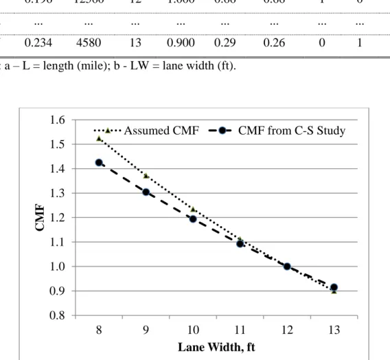
Table 1 below shows snapshots of the simulated crash counts for N segments considering a single variable of lane width. In this table, the CMF was assumed to be 0.9, which meant the increase of one foot in lane width decreased the predicted number of crashes by 10 percent (1.0 - 0.9), with the base condition for a lane width equal to 12 ft. So, the CMF specific to a segment i can be calculated as Equation 3-9. The assumed CM-Function for lane width is shown in Figure 1 (the dotted line with triangles).

26

Table 1 Example of Simulated Crash Counts for N Segments Seg. L a _{AADT LW} b _CMF spf N N_{true Yr 1 Yr 2 Yr 3} 1 0.113 15360 11 1.111 0.47 0.52 0 0 1 2 0.213 18420 8 1.524 1.05 1.60 1 3 2 3 0.125 4260 9 1.372 0.14 0.20 0 0 1 4 0.161 10600 10 1.235 0.46 0.56 1 0 1 5 0.196 12560 12 1.000 0.66 0.66 1 0 2 ... ... ... ... ... ... ... ... ... ... N 0.234 4580 13 0.900 0.29 0.26 0 1 1

Note: a – L = length (mile); b - LW = lane width (ft).

Figure 1 An Example Illustrating the Assumed CMF and CMF Derived from SPFs 0.8 0.9 1.0 1.1 1.2 1.3 1.4 1.5 1.6 8 9 10 11 12 13 CM F Lane Width, ft

27 The CMF for lane width is given by:

12 , 0.9 i i LW LW i CMF   (3-9) Where, i

LW = lane width of segment i (ft); and ,

i LW i

CMF = specific CMF for lane width of segment i.

Thus, the true crash mean of segment i was calculated as (recall that the calibration factor was assumed to be 1.0 for all segments in this study):

, , ,

true i spf i LW i

N N CMF (3-10)

Then, the exp( )_i of each segment was randomly generated based on a Gamma distribution with parameters mean equal to 1 and dispersion parameter equal to





, true i

N and exp( )_i , as shown in Equation 3-3b.

After, a sequence of Poisson counts were generated based on the mean  for each segment. Three years of simulated crash counts are shown in the last three columns in Table 1. The theoretical function form of these crash counts is shown in

Equation 3-11. 12 4 , , , 2.67 10 0.9 i LW true i spf i LW i i i N N CMF     L AADT  (3-11a) Or equivalently, 4 , 9.45 10 ( 0.105 ) true i i i i N     L AADTexp  LW (3-11b)

28

The simulated crash data was analyzed using the NB regression model. The mean functional form is provided in Equation 3-12.

1

0 2

( _i) _i ( _i)

E    L AADT exp  LW (3-12)

The coefficients of Equation 3-12 were estimated using a NB regression model in MASS package (Ripley et al. 2014) within the software R. The GOF measures were calculated using Metrics package (Hamner 2013). The modeling output is shown in Table 2. The p-values indicate the variables were statistically significant at the 99 percent level in this example. And, the small MAD and MSPE show the modeling result performed well (given the simulated data).

Based on the fitting result, the CM-Function for lane width derived from this SPF is shown in Equation 3-13. 12 2 [ ( 12)] 0.915LW LW CMF exp   LW   (3-13)

The value of 12 in Equation 3-13 reflects the base condition for lane width, which means that the CMF derived from prediction model is equal to 1.0. In this case, with an increment of one foot in lane width, the crash mean was expected to be multiplied by _e2 _{0.915. So, the CMF derived from the SPF was 0.915 in this}

29 Table 2 Modeling Output of the Example Data

Model Variable Theo. Value a _{Coef. Value} b _SE c _p-Value

Intercept [ln(



(9.45 10 )

ln   =-6.96 -6.810 0.340 5.3911E-89

Ln(AADT) (



Lane Width (



AIC 20614.5

MAD 0.214

MSPE 0.244

30

The bias between the assumed CMF and that from the SPF (without repeat in this example) is calculated as:

=CMF_Assumed CMF_SPF 0.90 0.915 0.015

     

And the error percentage is:

0.015 100 100 1.69(%) 0.90 Assumed bias e CMF      

By repeating the Steps 2 to 4 100 times, 100 CMFs could be estimated. The mean and standard deviation of CMFs and mean of GOF measures could be calculated. The estimation bias and error percentage were then calculated based upon the mean value of derived CMFs. For illustration purposes, this example only considered one variable, lane width.

3.1.3 Scenarios

Two scenarios were examined in Task 1 to accommodate more complex situations with different levels of dispersions (i.e., inverse dispersion parameters) and two additional variables, curve density and pavement friction. The scenarios are described below. The scenarios were names as “Scenario Number”. To make it consistent, the scenarios in the following tasks were given similar names, and the scenario numbers were continuous.

Scenario I: Consider one variable only, linear relationship

Various CMF values were assumed for lane width in this scenario. The objective was to examine whether or not the regression models can produce reliable CMFs when all the requirements of a cross-sectional study were satisfied.

31

Scenario II: Consider three variables, linear relationship

This scenario considered three variables, lane width, curve density and pavement friction. Details about the last two variables are introduced in Section 3.6.1. A fixed CMF value was assigned for each of the three variables. The objective was to examine whether the CMFs derived from SPFs were reliable when multiple variables were considered.

To reflect different traffic characteristics, the inverse dispersion parameter  in the two scenarios varied between 0.5, 1.0 and 2.0, respectively.

3.2 Omitted Variable Problem

As has been documented in Chapter 2, omitted variable is an important problem with regression models. This problem can lead to biased parameter estimates in the regression models and incorrect CMFs. This task investigated how the omitted-variable problem influenced the CMFs derived from regression models. In the previous section, all factors that influenced crash risk were assumed to be known. In contrast, not all the factors affecting crash risk were known or able to be captured by the model in this section. One scenario (i.e., Scenario III) was studied to address this problem, as described below.

Scenario III: Omitted variables, linear relationship

This scenario considered three variables, lane width, curve density and pavement friction. Their CMFs were assumed to be in linear forms, the same as that in Scenario II. But only one variable, the lane width, was included in the SPF; this fell under the

32

omitted-variable problem. The inverse dispersion parameter  in this scenarios also varied between 0.5, 1.0 and 2.0, respectively.

The methodology used to evaluate the quality of CMFs in this section was

essentially the same as that in Section 3.1, except that the two variables were excluded in the regression model.

3.3 Nonlinear Relationships

This section describes how the accuracy of CMFs derived from SPFs was investigated when some variables had nonlinear relationships. Intuitively, if the nonlinear relationship is weak (the CM-Function curve is quite flat or approximately a straight line), the accuracy of CMFs derived from SPFs should be similar to those in the previous scenarios. In the contrast, if the nonlinear relationship is strong (the curve is sharp), the accuracy of CMFs may be potentially affected. A measurement is necessary to describe how flat or sharp the curve is. This section first introduces the concept of quantifying nonlinearity, then presents the scenarios.

3.3.1 Quantifying Nonlinearity

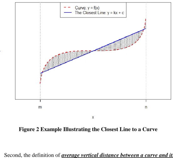
First, the definition of the closest line to a curve. For a given integrable curve

( )

y



f x

[ , ]

m n

y

  

k x c

y



f x

( )

y

  

k x c

33

between the two (the shadowed area in Figure 2). Given the range, in general, the larger the area is, the stronger the nonlinearity the curve tends to have. Particularly, if the given function is linear, the closest line is the function itself, and the area is technically equal to zero.

Figure 2 Example Illustrating the Closest Line to a Curve

Second, the definition of average vertical distance between a curve and its closest line. Although the area between a curve and its closest line can reflect the nonlinearity of the curve, the area still depends on the range. Wider range is more likely to yield larger area. The variables affecting traffic crashes are usually different in their possible values in practice. For example, the lane width may vary from 8 ft to 13 ft,

34

while the curve density may vary from 0 to 16 curves per mile. A standardized measurement is necessary to quantify the nonlinearity. The average vertical distance (AVD) between a curve and its closest line is defined as the area between the two divided by the range. So, in Figure 2, the AVD is calculated as dividing the shadowed area by nm. This way, the AVD itself can be used to quantify the nonlinearity of a curve regardless of its range. The larger this distance is, the stronger the nonlinearity that curve has. If the given function is linear, the AVD is zero.

The details for calculating the coefficients of the line (i.e., k and c) and AVD are shown below. The objective is to minimize the area, shown in Equation 3-14.

| ( ) ( ) | n m Area





k and c can be easily derived through mathematical translations, shown below.

2 2 ( ) ( ) ( ) ( ) [ ] n n n m m m n n m m n m xf x dx f x dx xdx k n m x dx xdx     























The area can be calculated by substituting k and c into Equation 3-14a, and the AVD is then calculated as dividing the area by nm. The AVD was used to measure

35 3.3.2 Scenarios

The method used to evaluate the accuracy of CMFs with nonlinear relationships with crash risk was similar with that of linear relationships. The only difference was that nonlinear CM-Functions were assumed for some variable(s) and used to generate crash counts. Three scenarios were analyzed in this section, as described below.

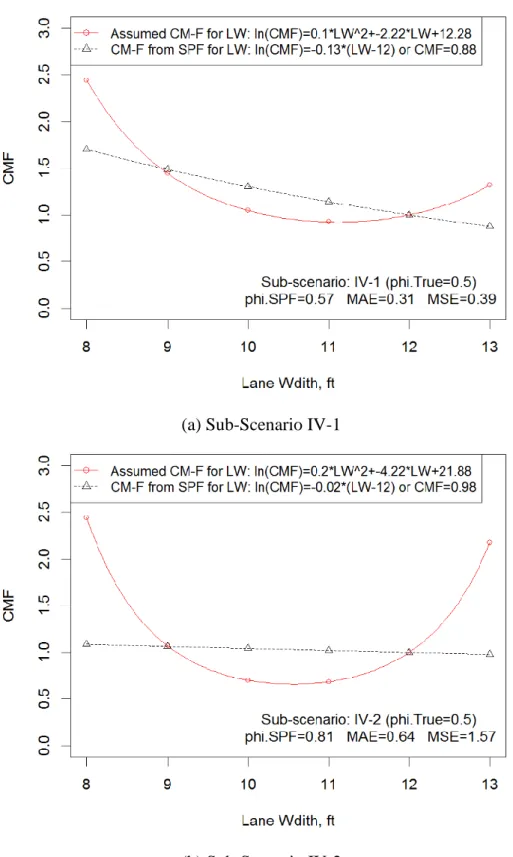
Scenario IV: Consider one variable only, in nonlinear form

Only lane width was considered and assumed to have nonlinear effects on crash. The main objective was to examine the bias of CMF for a variable with different levels of nonlinearity.

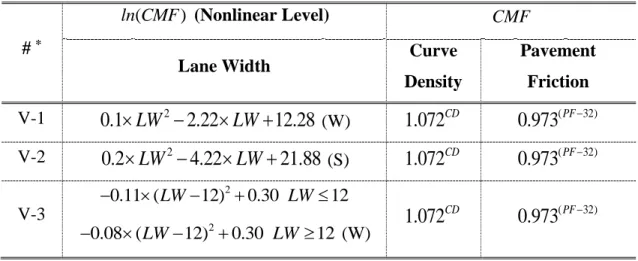
Scenario V: Consider three variables, only one in nonlinear form Three variables, lane width, curve density and pavement friction, were

considered in this scenario. Fixed CMFs were assigned to curve density and pavement friction. The CM-Functions for lane width were assumed to be in nonlinear forms. The main objective was to examine the influence of nonlinear variables on the accuracy of CMFs for linear variables.

Scenario VI: Consider three variables, two in nonlinear form

This scenario was similar with Scenario V, but both lane width and curve density were assumed to have nonlinear relationships. The CMF for pavement friction was fixed. The main objective was to examine the influence of nonlinear variables on the accuracy of CMFs for both linear and nonlinear variables.

36

For all the three scenarios, the assumed nonlinear relationships varied from weak to strong. Thus, each scenario contained a number of sub-scenarios. In addition, the inverse dispersion parameter  in each sub-scenario varied between 0.5, 1.0 and 2.0.

Note that, in Section 3.1, the theoretical functions for generating crash counts and the considered functional forms in regression models were of the same family (i.e., linear form or relationship). And the assumed CMFs and those generated from SPFs were similar (i.e., single ones). Only one bias and error percentage were calculated to examine the quality of CMFs. However, in this section, the theoretical functions were in nonlinear forms, which were not of the same family as the considered functional forms. No single CMF could be used to represent the assumed CM-Function. Thus, one bias or error percentage was not enough to assess the quality of CMFs. To overcome this problem, several specific CMFs for variables at typical points from both the assumed CM-Function and that developed from regression models were compared, and the bias and error percentage were calculated based on the specific CMFs.

3.4 Variable Correlation

In the previous sections, all the considered variables were assumed to be (perfectly) independent of each other, and each was uniformly or discrete uniformly distributed among the corresponding range (as will be shown in Section 3.6.1).

However, this might not be the case in practice. Some variables may be highly correlated with each other. For example, when constructing two highways, one with higher demand (i.e., AADT) and the other with lower, it is common that the former one will be designed

37

with higher standard, e.g., wider lanes and shoulders, etc. Thus, variables AADT and lane width are correlated. And also, in highway design manuals (AASHTO 2004; TxDOT 2014), lane width is recommended to be 12 ft for most highways. So 12 ft may be prevalent among lanes, and it is not discrete uniformly distributed in practices. This might affect the regression result and hence the CMFs for variables. This section aimed to examine whether or not variable correlation had influence on the CMFs derived from regression models. Two scenarios (i.e., Scenario VII and VIII) were analyzed, as

described below.

Scenario VII: Variable correlation, linear relationship

This scenario considered one variables, lane width, only. Various CMF values were assumed for lane width. This scenario was basically the same as Scenario I, except the variable lane width was correlated with AADT.

Scenario VIII: Variable correlation, nonlinear relationship

Only lane width was considered and assumed to have nonlinear effects on crash. This scenario was basically the same as Scenario V, except the variable lane width was correlated with AADT.

The inverse dispersion parameter  in the two scenarios varied between 0.5, 1.0 and 2.0, respectively. The methodology used to evaluate the quality of CMFs in this section was also essentially the same as that in Sections 3.1 and 3.3, except that two variables AADT and lane width were correlated. A new dataset was generated, as will be described in Section 3.6.2.

38 3.5 Combined Safety Effect

A similar approach was used to evaluate the CMFs derived from regression models considering the dependence of variables (not in a statistical sense), but it was modified to fit the specific characteristics of this task. The main concepts were:

(1) assume CMFs and dependence for variables; (2) generate random crash counts; and (3) estimate CMFs using regression models and compare them with the assumed true values.

The major difference in this section was the use of adjustment factors (AFs). An adjustment factor was assumed to capture the combination effect of multiple treatments. This was similar to the method used in the recent study by Park and Abdel-Aty (2015b). The combined CMF for multiple treatments is calculated by Equation 3-15.

_{1 1}  1    1 n X X_base X_n X_nbase n I X I X comb X X CMF CMF  CMF AF     (3-15) Where, comb

CMF = the combined CMF for a segment;

j

X

CMF = the assumed specific CMF for variable X_j of the segment;

AF

X = the base condition for variable X_j; and, Xj Xjbase

 

I _ X = indicator function for variable X_j. It equaled to zero if variable

j

39

The indicator functions made the adjustment factor to be working or not based on specific conditions of the segment and the presumed dependence relationships between variables.

To simplify the analysis, only two variables, lane width and shoulder width, were considered in this scenario (i.e., Scenario IX). And each variable in the dataset was assigned one of two values: the baseline and improved, respectively. For lane width, it was either 12 ft (baseline) or 13 ft (wider lane). And for shoulder width, it was either 6 ft (baseline) or 7 ft (wider shoulder). This way, the total segments could be classified into four categories: (1) baseline; (2) wider lane; (3) wider shoulder; and (4) wider lane and wider shoulder. They are described in Table 3.

The CMF for lane width was assumed to be CMFLW with baseline equal to 12 ft.

So, the specific CMFs for lane widths of 12 ft and 13 ft were 1.0 and CMFLW,

respectively. Similarly, the CMF for shoulder width was assumed to be CMFSW with

baseline equal to 6 ft. The specific CMFs for shoulder widths of 6 ft and 7 ft were 1.0 and CMFSW, respectively. This study assumed neither CMFLW nor CMFSW equaled to

1.0. Furthermore, the adjustment factor was used to capture the dependence of the safety effects of the two variables. That is to say, if a segment was wider in both lane and shoulder, the combined CMF was multiplied by the adjustment factor. The CMFs for lane width, shoulder width and combined CMF for the four groups of segments are shown in the last three columns of Table 3.

40 Table 3 Summary of Four Groups of Segments

Group LW (ft) SW (ft) CMF for LW CMF for SW Combined CMF Baseline 12 6 1.0 1.0 1.0 Wider Lane 13 6 CMFLW 1.0 CMFLW Wider Shoulder 12 7 1.0 CMFSW CMFSW

Wider Lane and

Wider Shoulder 13 7 CMFLW CMFSW CMFLW  CMFSW  AF Note: LW = lane width; SW = shoulder width.

Specifically, the assumed CMF for lane width (i.e., CMFLW) varied between 0.8

and 0.9. And that for shoulder width (i.e., CMFSW) varied between 0.85 and 0.9. The

adjustment factor changed from 0.80, 0.90, 0.95, 1.05, 1.10 to 1.20. When the adjustment factor is less than 1.0, it means widening both lane and shoulder width simultaneously will bring more safety benefits than the “sum” of the two single

treatments. The smaller the adjustment factor is, the more benefit will be. In contrast, if it is more than 1.0, taking the two treatments simultaneously will have a lower effect than their “sum.” The higher the adjustment factor is, the lower the combined safety effect will be.

In total, there were 24 sub-scenarios in this section, shown in Table 4. The inverse dispersion parameter () varied between 0.5, 1.0 and 2.0 in each sub-scenario to reflect different traffic characteristics.

The theoretical function of the generated crash counts in this scenario is shown in Equation 3-16.

41

4

, , , 2.67 10 ,

true i spf i comb i i i comb i

N N CMF     L AADT CMF (3-16)

Where, , true i

N = true crash mean for roadway segment i during a certain time period (i.e., one year);

i

AADT = AADT of segment i (vehicles per day); i

L = length of segment i (mile); and, ,

comb i

CMF = the combined CMF for lane width and shoulder width of segment i. It was calculated by the methods shown in Table 3 (the last column).

The CMFs for the two variables were derived from SPFs with similar procedures utilized in the previous study. The considered functional form is shown in

Equation 3-17, in which the two variables (i.e., lane width and shoulder width) were assumed to influence crashes independently.

1 0 2 3 ( _i) _i ( _{i i}) E    L AADT exp  LW   SW (3-17) Where, ( _i)

E  = the estimated crash mean during a period (i.e., one year) for segment i; i

LW = lane width of segment i (ft); i

SW = shoulder width of segment i (ft); and 0, 1, 2, 3

42

Table 4 Summary of Sub-Scenarios in Scenario IX

Sub-Scenario CMF for LW CMF for SW AF

IX-1 0.8 0.85 0.80 IX-2 0.8 0.85 0.90 IX-3 0.8 0.85 0.95 IX-4 0.8 0.85 1.05 IX-5 0.8 0.85 1.10 IX-6 0.8 0.85 1.20 IX-7 0.8 0.9 0.80 IX-8 0.8 0.9 0.90 IX-9 0.8 0.9 0.95 IX-10 0.8 0.9 1.05 IX-11 0.8 0.9 1.10 IX-12 0.8 0.9 1.20 IX-13 0.9 0.85 0.80 IX-14 0.9 0.85 0.90 IX-15 0.9 0.85 0.95 IX-16 0.9 0.85 1.05 IX-17 0.9 0.85 1.10 IX-18 0.9 0.85 1.20 IX-19 0.9 0.9 0.80 IX-20 0.9 0.9 0.90 IX-21 0.9 0.9 0.95 IX-22 0.9 0.9 1.05 IX-23 0.9 0.9 1.10 IX-24 0.9 0.9 1.20