On methods for prediction based on complex
data with missing values and robust principal
component analysis
Holger Cevallos Valdiviezo
Thesis to obtain the degree of Doctor in Statistical Data Analysis
Academic year 2016-2017
Promotor: Prof. Stefan Van Aelst
Faculty of Sciences
Department of Applied Mathematics, Computer science and Statistics Ghent University
Massale hoeveelheden gegevens worden momenteel geproduceerd op verbazingwekkende snelheid. Technologische ontwikkelingen maken het goedkoper en toegankelijk voor bedrijven/instellingen om grote stromen van data te verkrijgen of te genereren. Deze gegevens kunnen verschillende types van complexiteiten bevatten zoals niet-geobserveerde waarden, onlogische waarden, extreme waarnemingen, en vele anderen. Anderzijds er-varen onderzoekers soms beperkingen om steeproefgegevens te bekomen. Zo kan het kostbaar zijn om een organisme te laten groeien in een lab. Daarom kan een onderzoeker ervoor kiezen om er slechts enkele te laten groeien, ten koste van een lagere kwaliteit van de resultaten. Bij dit soort gegevens wordt vaak een groot aantal eigenschappen gemeten in slechts een klein aantal waarnemingen, zodat de dimensie van de data veel groter is dan de omvang. Denk bijvoorbeeld aan microarray data. Heel vaak zijn beoefe-naars meer bezorgd over de correcte inning van de gegevens dan het eigenlijke uitvoeren van een correcte data-analyse. In dit werk bespreken we methoden voor twee relevante stappen in de data-analyse. We kijken eerst naar methoden voor de verkennende stap waarbij de beoefenaar wil navigeren doorheen de grote stroom aan informatie in de data om te beginnen met het begrijpen van hun structuur en eigenschappen. Vervolgens bespreken wij methoden voor statistische data-analyse, gericht op een van de belangri-jkste taken in deze stap: het voorspellen van een uitkomst. In dit werk willen we ook vaak voorkomende complexiteiten van real data toepassingen zoals hoog-dimensionale gegevens, atypische data en ontbrekende waarden aanpakken. Meer specifiek begint het proefschrift met een bespreking van methoden voor hoofdcomponentenanalyse, n van de meest populaire experimentele technieken. Deze methoden zijn uitbreidingen van de klassieke benadering van hoofdcomponenten analyse die bestand zijn tegen atypische gegevens. Hoofdstuk 1 beschrijft de Multivariate S- en de Multivariate Least Trimmed Squares schatters voor de principale componenten en stelt een algoritme voor dat meer robuuste resultaten kan opleveren en computationeel sneller is voor hoog-dimensionale problemen dan bestaande algoritmen voor deze methoden en andere robuuste meth-oden. We tonen aan dat de overeenkomstige functionalen Fisher-consistent zijn voor elliptische verdelingen. Bovendien bestuderen we de robuustheidseigenschappen van de Multivariate S-schatter door zijn invloedsfunctie af te leiden. De Multivariate S- en de Multivariate Least Trimmed Squares schatters richten zich echter alleen op uitschi-etende observaties (casewise outliers), dit wil zeggen waarnemingen zijn ofwel regulier ofwel uitschietend. Hoofdstuk 2 introduceert een nieuwe methode voor principale com-ponenten waarvan aangetoond wordt dat ze beter tegen uitschietende metingen bestand is: de coordinatewise Least Trimmed Squares schatter. In het bijzonder kan ons voorstel
wise Least Trimmed Squares schatter zodat deze snel kan berekend worden in hogere dimensies. Bovendien introduceren wij de functionaalvorm van de schatter en tonen aan dat deze Fisher-consistent is voor elliptische verdelingen. Hoofdstuk 3 breidt deze drie methoden uit naar de setting met functionele gegevens en laat zien dat deze uitbreidin-gen de robuustheidskenmerken van de methoden in de multivariate setting behouden. Het laatste hoofdstuk van het proefschrift handelt over het maken van voorspellingen in aanwezigheid van ontbrekende gegevens. Om voorspellingen te maken gebruiken we boom-gebaseerde methoden. Bomen zijn een populaire data mining techniek die het mogelijk maakt om voorspellingen te maken over gegevens van verschillende aard en in aanwezigheid van ontbrekende waarden. We vergelijken de voorspellingsprestaties van boom-gebaseerde technieken als de beschikbare trainingsdata variabelen met ontbrek-ende waarden bevatten. De ontbrekontbrek-ende waarden worden ofwel behandeld met behulp van surrogaat beslissingen in de bomen ofwel door de combinatie van een imputatiemeth-ode met een boom-gebaseerde methimputatiemeth-ode. Zowel classificatie- als regressieproblemen wor-den beschouwd. Over het algemeen tonen onze resultaten dat voor kleinere fracties van ontbrekende gegevens een ensemble methode gecombineerd met surrogaat beslissin-gen of enkelvoudige imputatie volstaat. Voor matige tot grote fracties van ontbrek-ende waarden, tonen ensemble methoden op basis van voorwaardelijke inferentiebomen in combinatie met meervoudige imputatie de beste prestaties, terwijl voorwaardelijke bagging gebruikmakend van surrogaten een goed alternatief is voor hoog-dimensionale voorspelling problemen. Theoretische resultaten bevestigen de potentieel betere voor-spellingsprestaties van meervoudige imputatie ensembles.
First of all I would like thank to God, who under His Mercy, has allowed me to reach this important moment in my life. He has taught me that everything is possible and has confirmed His promise that He is with us everyday until the end.
I would like to thank my supervisor, Prof. Stefan Van Aelst, whose comments, expla-nations, and suggestions were valuable for the production of this work. Thank you for your patience and for having allowed me to have this enriching experience in which I have learned a lot and have shared knowledge with colleagues and professors from other universities and institutions. Likewise, I would like to thank Prof. Matias Salibian-Barrera for sharing his research ideas with me and for letting me work on them. Thank you also for letting me work with your computational facilities, they were of big help to get calculations faster and on time. I would like to take this opportunity to thank the other members of the examination committee, Prof. Luc Duchateau, Prof. Gentiane Haesbroeck, Prof. Tim Verdonck and Prof. Dries Benoit. Thank you very much for the effort you made for reading the entire thesis and for the very interesting comments I got from you all. They have improved the quality of this work. I would also like to thank Prof. Olivier Thas, who as the chairman of the examination committee, guided me in the process of getting all the administrative steps fulfilled to be able to defend my thesis.
I would like to give special thanks to my parents, who has supported me all the time. Gracias por escucharme, aconsejarme, estar pendiente todo el tiempo de mi, a la dis-tancia. Gracias por hacer el esfuerzo de venir hasta ac´a. Gracias mami por orar por mi todos los d´ıas, se que lo haces. Los amo mucho y le doy gracias a Dios por permitirme compartir estos momentos junto a ustedes. Les dedico especialmente esta tesis. Thank you my little brother Daniel and thank you Diana for having come as well. Los amo. Quisiera tambi´en agradecer a mis t´ıas: Elsy, Carmen, Azucena, Chela. Gracias por orar por mi y por apoyarme en mis metas. I would also like to give special thanks to my dear Ariana. Me has mostrado que el amor existe, que este todo lo soporta a pesar de todas las dificultades. No tengo palabras para agradecerte mi amor. Estar´e muy feliz de regresar a casa y de compartir este logro contigo. Te amo.
I would also like to thank the professors from the Department of Statistics of Ghent University for sharing their knowledge with us, the students. To my office mates, thank you for tolerating me. I know it is very difficult! Thanks to all my dear friends that I have met during my stay in Ghent. It is difficult to name them all, but I keep everyone of you in my heart.
Contents
Abstract ii
Acknowledgements iv
List of Figures ix
List of Tables xi
1 Robust multivariate subspace estimation for high-dimensional data 1
1.1 Introduction. . . 1
1.1.1 Classical PCA approach . . . 3
1.2 The Multivariate S-estimator for PCA (MVS) inRp . . . 4
1.2.1 The estimator. . . 4
1.2.2 The functional . . . 7
1.3 The Multivariate least trimmed squares estimator for PCA (MVLTS) in Rp 11 1.3.1 The estimator. . . 11
1.3.2 The functional . . . 12
1.4 The algorithm. . . 15
1.4.1 Strategy to find the global minimum . . . 17
1.4.2 Strategy to find a good local minimum. . . 17
1.5 Number of components. . . 19
1.6 Simulation study . . . 21
1.7 Simulations with high dimensional data . . . 27
1.8 Computational time . . . 28
1.9 Real data example . . . 30
1.10 Discussion and conclusions. . . 32
2 Coordinatewise subspace estimation for high-dimensional data 34 2.1 Introduction. . . 34
2.2 The coordinatewise S-estimator in Rp . . . 36
2.2.1 The estimator. . . 36
2.3 The coordinatewise LTS estimator in Rp . . . 38
2.3.1 The estimator. . . 38
2.3.2 The functional . . . 40
2.4 The algorithm. . . 41
2.5 Number of components. . . 43
2.6 Simulation study . . . 45
2.6.1 Results . . . 45
2.7 Real data examples . . . 48
2.7.1 Top gear data. . . 49
2.7.2 Octane data. . . 52
2.8 Discussion and conclusions. . . 55
3 Functional data setting 56 3.1 Introduction. . . 56
3.2 The Multivariate least trimmed squares estimator for PCA (MVLTS) in the functional setting. . . 57
3.2.1 The functional inH . . . 58
3.3 The Multivariate S estimator for PCA (MVS) in the functional setting . . 61
3.3.1 The functional inH . . . 61
3.4 Componentwise least trimmed squares estimator (CooLTS) in the func-tional setting . . . 62
3.4.1 The functional inH . . . 62
3.5 Simulation. . . 62
3.5.1 Simulation design. . . 63
3.5.2 Results . . . 68
3.6 Real data example . . . 70
3.6.1 Mortality data . . . 71
3.7 Discussion and conclusions. . . 73
4 Tree-based prediction on incomplete data using imputation or surro-gate decisions 75 4.1 Introduction. . . 75 4.2 Methodology . . . 79 4.2.1 Tree-based methods . . . 79 4.2.2 Imputation methods . . . 80 4.3 Theoretical properties . . . 85 4.4 Simulation study . . . 90
4.5 Results and Discussion . . . 95
4.5.1 Comparison of techniques . . . 97
4.5.2 Effects of sample size and dimension . . . 102
4.5.3 Initial imputation versus surrogates . . . 104
4.5.4 Computational issues . . . 105
4.6 Conclusions and Future work . . . 107
A Proofs of theorems and additional lemmas 110 B Additional tables 119 C Tree-based methods 123 C.1 Tree-based methods . . . 123
C.3 DGM for the Simulated dataset . . . 127
D Additional Figures 147
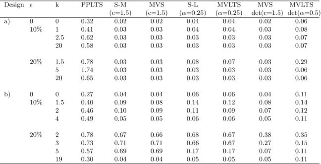
1.1 Relative unexplained variance to the best 2 dimensional subspace (epred)
as a function of kfor eigenvalue configuration a) and= 20%. . . 24
1.2 Relative unexplained variance to the best 2 dimensional subspace (epred)
as a function of kfor eigenvalue configuration b) and= 20%. . . 25
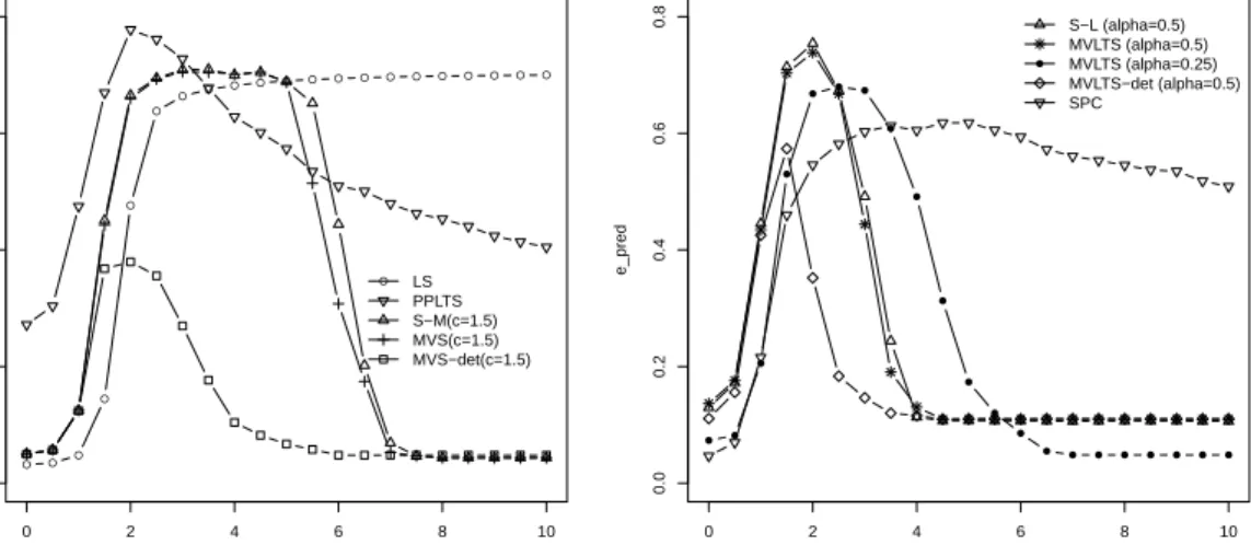
1.3 Mean estimation error eest as a function of kfor eigenvalue configuration
b) and = 20%.. . . 26
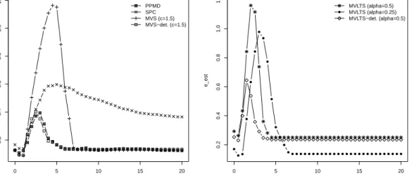
1.4 Mean relative prediction errorsepred for the simulations withp= 750 and
= 20% of contamination . . . 27
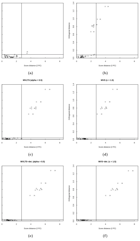
1.5 Diagnostic plots of the Octane dataset based on six two-dimensional PCA estimates. . . 31
2.1 Mean relative prediction errorsepredoverM = 200 replications as a
func-tion of the contaminafunc-tion valuesγ. Forγ = 0, theepredvalue is indicated
with the name of the method. Panels (a) to (d) shows the results with 5%, 10%, 15% and 20% of outlying cells. . . 46
2.2 Cell maps for selected rows of the Top gear data when detecting cellwise outliers withDetectDeviatingCells(left-hand side), with CooLTS (center) and with CooS (right-hand side). . . 51
2.3 Cell maps for the Octane dataset with n= 39 gasoline samples and p= 226 wavelengths: when detecting casewise outliers with a multivariate-PCA method (top panel), when using CooLTS (middle panel) and when using CooS (bottom panel). . . 54
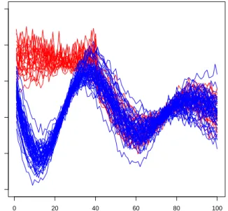
3.1 An example of Model 1 with1=2 = 0.30. Regular curves are shown in
blue color while contaminated curves are shown in red color . . . 65
3.2 An example of Model 2 with 1 = 0.3, 2 = 0.90. Regular curves are
shown in blue color while contaminated curves are shown in red color . . 66
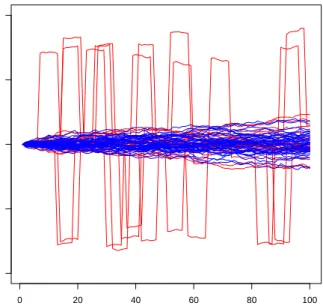
3.3 An example of Model 3 with = 0.30. Regular curves are shown in blue color while contaminated curves are shown in red color . . . 67
3.4 An example of Model 3 with = 0.90 and D = 1. Regular curves are shown in blue color while contaminated curves are shown in red color . . 67
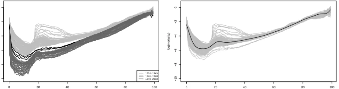
3.5 Mortality data. Panel (a) contains the curves for the years 1816 to 2010. Three periods can be distinguished and are marked with different gray scale colors. Panel (b) only depicts the curves corresponding to the period of interest from 1816 to 1948. On top the median curve is plotted. . . 71
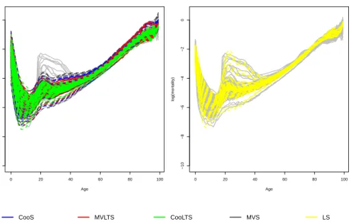
3.6 Robust approximations vs classical PCA approximations . . . 72
3.7 Outlier detection based on orthogonal distances . . . 72
3.8 Observed curves and PCA approximations by the methods analyzed for years of important events in France . . . 73
4.1 Mean MER results for the Survival data (top row) and Heart disease data (bottom row). Results are shown for data MCAR (left panel), MAR (middle panel) and MNAR (right panel). . . 99
4.2 Mean RMSPE results for the Fertility data (top row) and Birthweight data (bottom row). The values for the Birthweight dataset have been divided by 105. Results are shown for data MCAR (left panel), MAR (middle panel) and MNAR (right panel). . . 100
4.3 Mean RMSPE results for the simulated data. Results are shown for data MCAR (left), MAR (middle) and MNAR (right). . . 101
4.4 Effect of sample size on the prediction performance for simulated datasets under the MNAR mechanism. Results are shown for sample sizes with 750 observations (left panel), 1000 observations (middle panel) and 2000 observations (right panel) with dimension fixed at p= 10. . . 102
4.5 Effect of dimension on the prediction performance for simulated datasets under the MNAR mechanism. Results are shown for dimensions with 15 (left panel), 20 (middle panel) and 50 continuous predictors (right panel) with sample size fixed at N = 500. . . 103
4.6 Performance vs computation time for the Birthweight (top left), Heart (top right), Fertility (bottom left) and simulated (bottom right) datasets. The mean RMSPE values for the Birthweight dataset have been divided by 105. . . 106
4.7 A: Computation time vs sample size for simulated data; B: Computation time vs dimension for simulated data . . . 108
D.1 Cell maps for selected rows of the Top gear data: when detecting cellwise outliers with DetectDeviatingCells (left-hand side), when using CooLTS with deterministic starts (center) and when using CooS with deterministic starts (right-hand side). . . 148
D.2 Cell maps for the Octane dataset withn= 39 gasoline samples and p= 226 wavelengths: when detecting casewise outliers with a multivariate-PCA method (top panel), when using CooLTS with deterministic starts (middle panel) and when using CooS with deterministic starts (bottom panel). . . 149
1.1 Mean relative prediction errorsepred for the techniques with best
perfor-mance and for PPLTS . . . 24
1.2 Mean estimation errors eest for data without contamination . . . 25
1.3 Computational time in seconds as the dimensionp increases . . . 29
2.1 Mean relative prediction errorsepred for data without contamination . . . 47
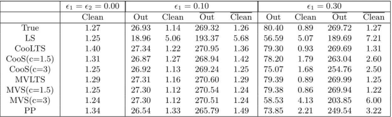
3.1 Mean prediction errors over 500 replications for Model 1 . . . 69
3.2 Mean prediction errors over 500 replications for Model 2 . . . 69
3.3 Mean prediction errors over 500 replications for Model 3 . . . 69
3.4 Mean prediction errors over 500 replications for Model 3 . . . 70
4.1 Overview of the 26 techniques investigated in this study. Each mark ‘×’ corresponds to a technique. The second mark in the MIST + RF box corresponds to a special case of this technique that consists of imputing bootstrap samples by MIST + RF. N/I stands for “not implemented”. . . 79
4.2 Number of observations and predictors listed for each dataset used in this study . . . 92
4.3 R function and its corresponding package name, package reference paper and settings for the implementation of each of the methods included in this study . . . 96
4.4 Ranges of mean relative improvement for single imputation over all tech-niques and missing data fractions. Note that the first result line corre-sponds to the MCAR pattern, the second to the MAR and the third to the MNAR pattern. Only CondRF, CondTree and CART were taken into account for these comparisons. . . 104
4.5 Ranges of mean relative improvement for multiple imputation with Con-dRF vs ConCon-dRF with surrogates over all missing data fractions. Note that the first result line corresponds to the MCAR pattern, the second to the MAR and the third to the MNAR pattern. . . 105
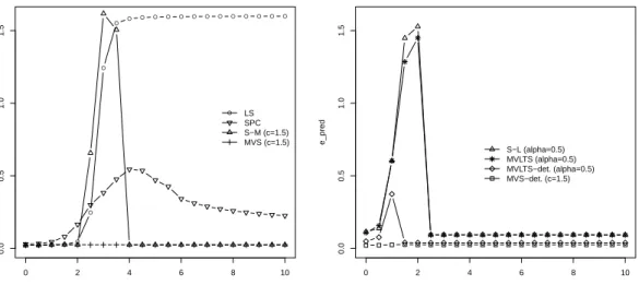
B.1 Additional results for LS, S-M, S-L, PPMD and PPME in the simulation study of section 1.6 . . . 119
B.2 Additional results for PPLTS, SPC, MVS and MVLTS in the simulation study of section 1.6 . . . 120
B.3 Additional results for MVS and MVLTS computed with the algorithm with deterministic starts in the simulation study of section 1.6 . . . 120
B.4 Mean prediction errors over 500 replications for Model 1 . . . 121
B.5 Mean prediction errors over 500 replications for Model 2 . . . 121
B.6 Mean prediction errors over 500 replications for Model 3 . . . 122 xi
B.7 Mean prediction errors over 500 replications for Model 3 . . . 122
C.1 Summary of mean MSPE/MER values for the real-life datasets. The values for the Birthweight dataset have been divided by 104. Results of techniques with prior kNN imputation, Bagging and MIST imputed bootstrap samples + RF are not shown here. Missing data was induced under MCAR, MAR and MNAR patterns at different fractions and fol-lowing 2 schemes: all p variables (p−1 for MAR) with missing values (1/1) and only p/3 variables with missing values (1/3). Note that the first result line of each technique corresponds to the MCAR pattern, the second to the MAR and the third to the MNAR pattern. N/I stands for “not implemented”.. . . 128
C.2 Summary of mean MSPE/MER values for the simulated dataset. Results of techniques with prior kNN imputation, Bagging and MIST imputed bootstrap samples + RF are not shown here. Missing data was induced under MCAR, MAR and MNAR patterns at different fractions and fol-lowing 2 schemes: 8 variables with missing values and only 8/3 variables with missing values. Note that the first result line of each technique cor-responds to the MCAR pattern, the second to the MAR and the third to the MNAR pattern. N/I stands for “not implemented”. . . 129
C.3 For each real-life dataset analyzed, we show the average percentage of missing data and the average percentage of complete observations across 1,000 simulations in which missingness is introduced according to a fixed pattern, fraction and scheme of missing values. . . 130
C.4 For the simulated dataset, we show the average percentage of missing data and the average percentage of complete observations across 1,000 simu-lations in which missingness is introduced according to a fixed pattern, fraction and scheme of missing values. . . 131
C.5 Summary of mean MER values for the Survival dataset. Missing data was induced under MCAR, MAR and MNAR patterns at different fractions and following 2 schemes: allp= 3 =m variables with missing values (for MAR pattern: m=p−1 = 2) and onlyp/3 variables with missing values. N/I stands for “not implemented”. . . 132
C.6 Summary of standard error (SE) estimates of each of the MER estimates for the Survival dataset. Missing data was induced under MCAR, MAR and MNAR patterns at different fractions and following 2 schemes: all p = 3 = m variables with missing values (for MAR pattern: m = p−
1 = 2) and only p/3 variables with missing values. N/I stands for “not implemented”. . . 133
C.7 Summary of mean relative improvement values with an imputation strat-egy compared to surrogate decisions through different missing data sce-narios for the Survival dataset. Only CondRF, CondTree and CART were taken into account for these comparisons (because RF implementation in R -randomForest()- cannot be fitted on incomplete data). Missing data was induced under MCAR, MAR and MNAR patterns at different frac-tions and following 2 schemes: allp= 3 =mvariables with missing values (for MAR pattern: m =p−1 = 2) and only p/3 variables with missing values. . . 134
C.8 Summary of mean MER values for the Heart dataset. Techniques with priorkNN imputation could not be fitted since this dataset contains cat-egorical predictors. Missing data was induced under MCAR, MAR and MNAR patterns at different fractions and following 2 schemes: all p = 13 =mvariables with missing values (for MAR pattern: m=p−1 = 12) and only p/3 variables with missing values. N/I stands for “not imple-mented”.. . . 135
C.9 Summary of standard error (SE) estimates of each of the MER estimates for the Heart dataset. Techniques with priorkNN imputation could not be fitted since this dataset contains categorical predictors. Missing data was induced under MCAR, MAR and MNAR patterns at different fractions and following 2 schemes: all p = 13 = m variables with missing values (for MAR pattern: m=p−1 = 12) and onlyp/3 variables with missing values. N/I stands for “not implemented”. . . 136
C.10 Summary of mean relative improvement values with an imputation strat-egy compared to surrogate decisions through different missing data sce-narios for the Heart dataset. Only CondRF, CondTree and CART were taken into account for these comparisons (because RF implementation in R -randomForest()- cannot be fitted on incomplete data). In addition, kNN imputation could not be implemented since this dataset contains categorical predictors. Missing data was induced under MCAR, MAR and MNAR patterns at different fractions and following 2 schemes: all p= 13 =mvariables with missing values (for MAR pattern: m=p−1 = 12) and only p/3 variables with missing values. . . 137
C.11 Summary of mean MSPE values for the Fertility dataset. Missing data was induced under MCAR, MAR and MNAR patterns at different frac-tions and following 2 schemes: allp= 5 =mvariables with missing values (for MAR pattern: m =p−1 = 4) and only p/3 variables with missing values. N/I stands for “not implemented”. . . 138
C.12 Summary of standard error (SE) estimates of each of the MSPE estimates for the Fertility dataset. Missing data was induced under MCAR, MAR and MNAR patterns at different fractions and following 2 schemes: all p = 5 = m variables with missing values (for MAR pattern: m = p−
1 = 4) and only p/3 variables with missing values. N/I stands for “not implemented”. . . 139
C.13 Summary of mean relative improvement values with an imputation strat-egy compared to surrogate decisions through different missing data sce-narios for the Fertility dataset. Only CondRF, CondTree and CART were taken into account for these comparisons (because RF implementation in R -randomForest()- cannot be fitted on incomplete data). Missing data was induced under MCAR, MAR and MNAR patterns at different frac-tions and following 2 schemes: allp= 5 =mvariables with missing values (for MAR pattern: m =p−1 = 4) and only p/3 variables with missing values. . . 140
C.14 Summary of mean MSPE values for the Birthweight dataset. Techniques with priorkNN imputation could not be fitted since this dataset contains categorical predictors. Missing data was induced under MCAR, MAR and MNAR patterns at different fractions and following 2 schemes: allp= 8 = m variables with missing values (for MAR pattern: m =p−1 = 7) and only p/3 variables with missing values. N/I stands for “not implemented”.141
C.15 Summary of standard error (SE) estimates of each of the MSPE estimates for the Birthweight dataset. Techniques with priorkNN imputation could not be fitted since this dataset contains categorical predictors. Missing data was induced under MCAR, MAR and MNAR patterns at different fractions and following 2 schemes: all p = 8 =m variables with missing values (for MAR pattern: m = p−1 = 7) and only p/3 variables with missing values. N/I stands for “not implemented”. . . 142
C.16 Summary of mean relative improvement values with an imputation strat-egy compared to surrogate decisions through different missing data sce-narios for the Birthweight dataset. Only CondRF, CondTree and CART were taken into account for these comparisons (because RF implemen-tation in R -randomForest()- cannot be fitted on incomplete data). In addition, kNN imputation could not be implemented since this dataset contains categorical predictors. Missing data was induced under MCAR, MAR and MNAR patterns at different fractions and following 2 schemes: all p = 8 = m variables with missing values (for MAR pattern: m = p−1 = 7) and only p/3 variables with missing values. . . 143
C.17 Summary of mean MSPE values for the simulated dataset. Missing data was induced under MCAR, MAR and MNAR patterns at different frac-tions and following 2 schemes: 8 variables with missing values and only 8/3 variables with missing values. N/I stands for “not implemented”. . . 144
C.18 Summary of standard error (SE) estimates of each of the MSPE estimates for the simulated dataset. Missing data was induced under MCAR, MAR and MNAR patterns at different fractions and following 2 schemes: 8 variables with missing values and only 8/3 variables with missing values. N/I stands for “not implemented”. . . 145
C.19 Summary of mean relative improvement values with an imputation strat-egy compared to surrogate decisions through different missing data sce-narios for the simulated dataset. Only CondRF, CondTree and CART were taken into account for these comparisons (because RF implementa-tion in R -randomForest()- cannot be fitted on incomplete data). Missing data was induced under MCAR, MAR and MNAR patterns at different fractions and following 2 schemes: 8 variables with missing values and only 8/3 variables with missing values. . . 146
Robust multivariate subspace
estimation for high-dimensional
data
The content of this chapter is work in progress for future publication.
1.1
Introduction
Principal component analysis (PCA) is a popular exploratory tool for multivariate data. Classical principal component analysis can be formulated in several ways. One such formulation is as follows. Classical PCA aims to find an optimal lower-dimensional subspace in the sense of minimizing the mean of the squared euclidean distances be-tween the original observations and their orthogonal projections onto the subspace. It is well-known that the directions spanning this optimal subspace correspond to the first eigenvectors of the sample covariance matrix. Hence, classical PCA also finds the di-rections of maximum variability of the data. PCA estimates are often used to visualize multivariate data and to quickly learn about the main sources of variation in the data. However, this classical approach to PCA is very sensitive to atypical data. In particular, the subspace found by minimizing the squared error loss can easily be pulled towards outliers.
There have been several proposals to robustify PCA. The earliest and easiest approach consists of taking the eigenvectors and eigenvalues of a robust scatter estimate instead of the standard sample covariance matrix. M-estimates, minimum volume ellipsoid (MVE) and S-estimates have been proposed for this purpose. However, this approach cannot
be used for high-dimensional data because calculating high-dimensional robust scatter matrices is computationally complex. Moreover, while the effciency of robust scatter estimators increases with dimension (that is, their variance at elliptical distributions decreases), this comes at the expense of a loss of robustness. Therefore,Locantore et al.
(1999) introduced spherical PCA which uses the covariance matrix of the data projected onto the unit sphere and can be calculated fast. Another alternative obtains robust PCA estimates by finding univariate directions that maximize a robust estimator of scale and are orthogonal to each other. This approach is known as robust projection pursuit (PP) and has been studied by Li and Chen (1985); Hubert et al. (2005) for example. A combination of both PP and robust scatter estimation was proposed by Hubert et al.
(2005).
Instead of looking for one direction at a time as in PP, one can seek an optimal lower-dimensional subspace directly. To this end,Liu et al.(2003) replaced the squared error loss of classical PCA by the absolute value of the errors. Croux et al.(2003) proposed a weighted version of this procedure to reduce the effect of high-leverage points. Maronna
(2005) considered robustly estimating the best lower-dimensional linear manifold by minimizing either an M-estimator of scale or a least trimmed squares (LTS) scale of the euclidean distances. Maronna called these approaches S-M and S-L and proposes an iterative algorithm to compute the solutions. He characterizes the solution by all directions orthogonal to the subspace and shows that these directions correspond to the eigenvectors associated with the smallest eigenvalues of a weighted covariance matrix. This may be a potential disadvantage when looking for a small dimensional subspace of high-dimensional data. In that case a high dimensional covariance matrix is still needed and a large number of eigenvectors is required. Computing all these directions in high-dimensional settings will take more time compared to computing only the first few directions comprising the subspace. Croux et al. (in press) investigated theoretical properties of the Maronna(2005) method based on the LTS scale.
In this chapter we re-investigate the methods of Maronna (2005) based on M and LTS scales, which we call Multivariate S-estimator and Multivariate least trimmed squares estimator respectively. We start with a short review of relevant properties of classical PCA in Section 1.1.1. We then give the definition of the Multivariate S-estimator esti-mator and corresponding estimating equations in section 1.2. Here, we also introduce the functional corresponding to the estimator. We show that the functional is Fisher-consistent at elliptical distributions and derive its influence function. In section 1.3we give the definition of the Multivariate least trimmed squares estimator and introduce the corresponding functional. We show that the functional is Fisher-consistent at el-liptical distributions. In section 1.4 algorithms for both estimators are proposed that are better suited for high-dimensional data. These algorithms directly determine the
directions of the low-dimensional optimal subspace rather than a basis of directions or-thogonal to the subspace. Moreover, our iterative algorithm uses estimating equations derived from first order conditions in order to update these directions, instead of com-puting high-dimensional covariance matrices as in the algorithm proposed by Maronna
(2005). These modifications make it possible to calculate the S-M and S-L solutions faster in high-dimensional settings. We consider two choices for the starting values. The first uses random initial orthogonal matrices as in Maronna (2005) and aims to find the global minimum. The second uses a few deterministic starting values inspired by
Hubert et al. (2012) and then finds the best local minimum that can be reached from these initial robust starting solutions. With deterministic starting values the algorithm is certainly faster and can make it feasible to calculate the solutions for even larger high-dimensional data. However, this approach is only useful if it does not jeopardize its performance. Section 1.5 discusses a fast strategy to choose the dimension of the subspace based on the proportion of unexplained variability. Finally, in section 1.6 we compare the performance of both algorithms through an extensive simulation study and a real data application.
1.1.1 Classical PCA approach
We first formalize our approach to the classical PCA problem. Consider a sampleZn=
{xi, i= 1, . . . , n} ⊂Rp and denote the corresponding data matrix by X= (x1. . .xn)t. Let x(Zn) = n1 Pni=1xi and Σb(Zn) = n−11
Pn
1(xi−x)(xi−x)T be the corresponding sample mean and sample covariance matrix. In this work, we consider principal com-ponent analysis as a method that looks for q < p orthogonal unit vectors b(l) ∈ Rp, 1≤l≤q, which span the linear subspace that gives the best approximation to the data set Zn. Let Bq ∈ Rp×q be an orthogonal matrix with columns Bq = (b(1), . . . ,b(q)), i.e. BTqBq = Iq, and rows bTj, j = 1, . . . , p. Let Aq ∈ Rn×q be the matrix with rows
aTi , i = 1, . . . , n, and m ∈ Rp. The corresponding approximations of the
observa-tions are given by bxi(Bq,Aq,m) ≡ bxi = m+Bqai, or elementwise ˆxij = mj +a T i bj. The associated multivariate residuals are given by ri = xi −bxi ∈ R
p. Its Euclidean norm, i.e. the Euclidean distance between xi and its approximation bxi, is denoted by
di(Bq,Aq,m) =di =krikRp. The classical principal components solution is now found
by minimizing min Bq,Aq,m n X i=1 kxi−bxi(Bq,Aq,m)k 2 Rp =Bmin q,Aq,m n X i=1 d2i(Bq,Aq,m) (1.1)
over allBq ∈Rp×q orthogonal,Aq∈Rn×q andm∈Rp. The solution to this problem is
matrix such that Bbq(Zn)TΣb(Zn)Bbq(Zn) = Λb(Zn) = diag(bλ1(Zn),bλ2(Zn), . . . ,bλq(Zn)), where bλ1(Zn) ≥ bλ2(Zn) ≥ . . . ≥ bλq(Zn) ≥ 0 are the q largest eigenvalues of Σb(Zn). Then, the solution to (1.1) is given by BbLS = Bbq(Zn), mbLS = x(Zn) and AbLS whose rows are given by baTi,LS = (xi −mbLS)
T b
Bq(Zn), i = 1, . . . , n. Note that the vectors
b
ai,LS are the scores of the observations xi on the columns of BbLS. If we assume that b
λq(Zn)>bλq+1(Zn) then the PCA solution is unique (see Seber, 1984, Theorem 5.3).
Unfortunately, classical principal component analysis can be very sensitive to the pres-ence of outliers. Since classical PCA is a least squares problem, outliers can pull the PCA subspace towards them. As a result, incorrect approximations for the regular data are obtained while the outliers cannot be detected because they do not appear as atypical points with unusually large Euclidean distance from the estimated subspace. Therefore, it is crucial to investigate approaches for PCA that can better resist the effect of these outliers.
1.2
The Multivariate S-estimator for PCA (MVS) in
R
p1.2.1 The estimator
From (1.1) it is easy to see that the classical PCA solution is found by minimizing a scale estimate σb
2(d(B
q,Aq,m)) of the Euclidean distances of the residuals d(Bq,Aq,m) = (d1, . . . , dn), given by b σ2(d(Bq,Aq,m)) = 1 n n X i=1 d2i(Bq,Aq,m). (1.2)
This classical scale estimator based on a quadratic loss function is clearly not robust against outliers. Maronna (2005) proposed to robustify the classical approach by re-placing bσ by an M-estimator of scale which is defined as follows. For a real vector u= (u1, u2, . . . , un) an M-scale estimatorbσM(u) is the solution inswhich satisfies
1 n n X i=1 ρc ui s =b (1.3)
where ρc(t) = ρ(t/c) with c >0 and where ρ :R → R+ is an even function such that
ρ(0) = 0 and ρ(t) is nondecreasing for t >0 (see e g. Maronna(2005)). The constantsc
and b are tuning parameters which can be chosen by the user. These constants control consistency and robustness/efficiency of the estimator. For instance with c = 1.54764 andb= 0.5 the estimator is consistent at the normal distribution and has the maximum breakdown point of 50%.
The multivariate S-estimator for PCA can now be defined as the solution (BbMVS,AbMVS,mbMVS) of the minimization problem
min
Bq,Aq,mb
σM(d(Bq,Aq,m)), (1.4)
where Bq ∈ Rp×q again needs to be an orthogonal matrix (i.e. BTqBq = Iq), and
b
σM(d(Bq,Aq,m)) is the solution in sof the equation
1 n n X i=1 ρc di(Bq,Aq,m) s =b. (1.5)
Note that in Maronna (2005) the Euclidean distance between each observation xi and its projection bxi onto theq-dimensional subspace is measured in the p−q dimensional orthogonal subspace which is equivalent to our current formulation in thep-dimensional space. We now write the MVS estimator defined in (1.4) in terms of the corresponding linear subspaces. Let Lb
b
BMVS be the q−dimensional linear subspace spanned by the
columns ofBbMVS. That is,Lb
b BMVS is the minimizer of min dim(LBq)=q b σM(d(LBq)) (1.6)
over all linear subspaces LBq of dimension q where d(LBq) = (d1(LBq), . . . , dn(LBq))
are the Euclidean distances to the subspace andσbM(d(LBq)) is the solution insof (1.5)
analogous to bσM(d(Bq,Aq,m)).
By implicitly differentiating the M-scale in (1.5) we obtain first order conditions for the MVS estimator which will be useful to develop an iterative procedure to find local minima of the MVS optimization problem. Let us denote the coordinates of the multivariate residuals ri by rij =xij−mj−aTi bj such that
di(Bq,Aq,m) =kxi−m−Bqaik= p X j=1 (xij−mj−aTi bj)2 1/2 . (1.7)
Then, the derivatives of bσM with respect toai,bj and mj become ∂σbM ∂ai =− Pp j=1ρ0 di b σM b σM di rijbj Pn i=1ρ0 di b σM di , i= 1, . . . , n , ∂σbM ∂bj =− Pn i=1ρ0 di b σM b σM di rijai Pn i=1ρ0 di b σM di ∂σbM ∂mj =− Pn i=1ρ 0di b σM b σM di rij Pn i=1ρ0 di b σM di , j= 1, . . . , p .
By setting the above equations to zero and writing
wi =ρ0 di b σM b σM di (1.8)
we obtain the following estimating equations:
p X j=1 (xij −mj)bj = p X j=1 bjbTj ai, 1≤i≤n , (1.9) n X i=1 wi(xij−mj)ai = n X i=1 wiaiaTi ! bj, (1.10) n X i=1 wi(xij−aTi bj) = n X i=1 wimj, 1≤j ≤p. (1.11)
These estimating equations naturally suggests an iterative reweighted least squares pro-cedure to converge to local minima of the objective function which will be used in our algorithm of the estimator. From (1.9) we obtain thatai=BTq(x−m). Hence, once Bq and m are known, the corresponding scores ai of the observations are easily obtained. By combining this with (1.11) we can also see that m = Pn
i=1wixi/( Pn
i=1wi). Note that if we put wi = 1 for all observations, then the solution of these equations becomes the classical PCA solution.
By combining the estimating equations it can also be seen that the MVS-PCA solutions (BbMVS,mbMVS) satisfy the equation:
n X i=1 wi(xi−mbMVS)(xi−mbMVS) T b BMVS=BbMVSΛb (1.12) where Λ =b BbTMVS Pn i=1wi(xi −mbMVS)(xi −mbMVS) T b BMVS and wi is given in (1.8).
From (1.12) it follows that the columns ofBbMVS can be taken as the firstq eigenvectors of the weighted covariance matrixC(mbMVS,BbMVS):
C(mbMVS,BbMVS) = 1 n n X i=1 wi(xi−mbMVS)(xi−mbMVS) T, (1.13)
This is in accordance with expression (9) inMaronna (2005).
1.2.2 The functional
To investigate asymptotic properties of the MVS estimator, we first introduce the func-tional corresponding to the estimator. Consider ap-dimensional random variablexwith a continuous distributionG. We assume that the distributionGhas location parameter
µand dispersion parameterΣ∈SPSD(p), i.e. Σbelongs to the class of symmetric posi-tive semi-definite matrices of sizep. It follows thatΣcan be decomposed asΣ=βΛβT
where Λ = diag(λ1, λ2, . . . , λp) with λ1 ≥ λ2 ≥ . . . ≥ λp ≥ 0 and β is an orthogonal
p×p matrix with columnsβ(1), . . . ,β(p).
Similarly as for the MVS estimator, the MVS functionals mMVS(G), BMVS(G) and aMVS(G) satisfy aMVS(G) = BTMVS(G) (x−mMVS(G)). To simplify notation, in what follows we drop G from the functionals. Therefore, we now focus on the functionals (mMVS,BMVS) which are the solution of the minimization problem
min m,BT qBq=Iq σM(dG(x,m,Bq)), (1.14) wheredG(x,m,Bq) = x−m−BqBTqx
and the M-scale functional σM satisfies Z ρ dG(x,m,Bq) σM(dG(x,m,Bq)) dG(x) =b (1.15)
The MVS functional can be written in a more general way as follows. Given an orthogo-nal matrixBq, letLBq be theq−dimensional linear space spanned by the columns ofBq.
To simplify the presentation, assume that the functional mMVS is known. In addition, denote as π(y,LBq) the orthogonal projection of y onto the subspace LBq. Therefore, the MVS functionalLBMVS corresponding to the definition in (1.6) is the solution of the
minimization problem
min
dim(LBq)=q
σM(dG(x,LBq)), (1.16)
over all linear subspacesLBq of dimensionq, wheredG(x,LBq) =
x−m−π(x−m,LBq) and the M-scale functionalσM satisfies (1.15) for dG(x,LBq).
An analogous derivation as for (1.13) shows that the columns of the functionalBMVScan be taken as the firstqeigenvectors of the weighted covariance matrixC(G,mMVS,BMVS) which is defined as:
C(G,mMVS,BMVS) = Z w(x−mMVS)(x−mMVS)TdG(x) (1.17) with weights w=ρ0 dG(x,mMVS,BMVS) σM(dG(x,mMVS,BMVS)) σM(dG(x,mMVS,BMVS)) dG(x,mMVS,BMVS) and MVS location functional
mMVS= R
wxdG(x) R
w dG(x)
Without loss of generality we can assume thatµ=0. We consider the case wherexhas a model distribution G=FΣwith density
fΣ(x) =
g(xTΣ−1x) p
det(Σ) , (1.18)
The function g is assumed to have a strictly negative derivative g0 such that FΣ is a
unimodal elliptically symmetric distribution around the origin (µ =0). To guarantee uniqueness of the best q−dimensional subspace Lq spanned by the columns of βq = (β(1), . . . ,β(q)), we need a condition on the eigenvalues of Σ. In particular, we need that λq > λq+1. The other eigenvalues may have the same value. Using (1.17) it can now be shown that the MVS-PCA functionalLBMVS(G) is Fisher-consistent at unimodal
elliptical distributionsFΣ.
Theorem 1.1. Letx∼FΣ, ap-dimensional elliptically distributed random variable with
location 0 and scatter Σ such that Σ = βΛβT where Λ = diag(λ1, λ2, . . . , λp), λ1 ≥
λ2≥. . .≥λp, and β is an orthogonal matrix with columnsβ(1), . . . ,β(p). Denote as Lq the linear space spanned by β(1), . . . ,β(q). Assume that λq > λq+1. Then, LBMVS(FΣ)
is a Fisher-consistent functional for Lq at the model distribution FΣ, i.e.
LBMVS(FΣ) =Lq (1.19)
In order to assess the effect on the estimator of a small amount of contamination at a single point we derive the influence function of the corresponding functional. More specifically, the influence function of a functional T at a distribution G measures the effect on T of an infinitesimal contamination at a single point Hampel et al. (1986). Let us denote the point mass at a point x0 by ∆x0 and consider the contaminated
distributionG,x0 = (1−)G+∆x0, then the influence function is given by IF(x0, T, G) = lim →0 T(G,x0)−T(G) = ∂ ∂T(G,x0)|=0. (1.20)
Let us assume w.l.o.g. thatµis known. We consider the influence function ofBMVS(G) at elliptical distributions. Let us assume, without loss of generality, that the columns of the functionalBMVS(G) are ordered according to decreasing eigenvalues. To derive this influence function we start with the influence function for the functional C(G,BMVS) defined in (1.17). To simplify notation let us write C(G) = C(G,BMVS), BMVS = BMVS(G) and σS =σM(dG(x,BMVS)), the S-scale functional. Moreover, let b(MVSj) de-note the jth column of BMVS, j = 1, . . . , q. Recall that b(MVSj) is thejth eigenvector of the weigthed covariance matrixC(G). Furthermore, letλj(G) denote thejth eigenvalue ofC(G). It can easily be seen that the MVS-PCA functionalBMVSis orthogonal equiv-ariant. Therefore, it suffices to compute the influence function at elliptical distributions
FΣwhere µ=0 and Σis a diagonal matrix.
Theorem 1.2. Let FΣ be a p-dimensional elliptical distribution with location µ = 0
and scatter Σ= diag(λ1, λ2, . . . , λp). For the diagonal elements of C(FΣ) it holds that:
IF(x0,C, FΣ)ii=u dFΣ(x0,BMVS) σS x20i−λi(FΣ) −EFΣ u0 dFΣ(x,BMVS) σS dFΣ(x,BMVS)x 2 i ·IF(x0, σS, FΣ) σ2 S , (1.21)
where u(t) =ρ0(t)/t and the IF of the S-scale functional σS is given by
IF(x0, σS, FΣ) = σ2SρdFΣ(x0,BMVS) σS −b 2b−2bσS+σS2EFΣ h ρ0dFΣ(x,BMVS) σS dFΣ(x,BMVS) i.
For the (i, j) elements with i= 1, . . . , q, j=q+ 1, . . . , p, we have that
IF(x0,C, FΣ)ij = [λj(FΣ)−λi(FΣ)]·u d FΣ(x0,BMVS) σS x0ix0j λj(FΣ)−λi(FΣ)−Hij(BMVS) . (1.22)
For the (i, j) elements with i=q+ 1, . . . , p, j= 1, . . . , q, we have that
IF(x0,C, FΣ)ij = [λj(FΣ)−λi(FΣ)]·u d FΣ(x0,BMVS) σS x0ix0j λj(FΣ)−λi(FΣ) +Hij(BMVS) . (1.23)
Finally, for the(i, j) elements with i= 1, . . . , q andj= 1, . . . , q, or withi=q+ 1, . . . , p and j=q+ 1, . . . , p such thati6=j, we have that
IF(x0,C, FΣ)ij =u dFΣ(x0,BMVS) σS x0ix0j, (1.24) with dFΣ(x0,BMVS) =kx0−BMVSB T
MVSx0k. Finally, the expression for Hij(BMVS) is
given in the Appendix.
Note that the influence functions are not bounded. However, they are non-increasing which means that the effect of a pointx0 on the MVS-PCA functional decreases as the distance from the point to its projectionBMVSBTMVSx0 on the subspace increases. Thus, only good leverage points, i.e. outliers in the direction of the linear subspace, may have a large influence on the estimator. On the other hand, the influence of outliers w.r.t. the subspace is bounded, and smoothly redescends to zero for the non-diagonal elements.
Using the theorem above, one can immediately obtain the influence functions for the columns of BMVS, i.e. the eigenvectors of C(FΣ). Note that with the assumption of
a diagonal Σ with distinct eigenvalues, it follows from the proof of Theorem 1.1 in Appendix A that BMVS(FΣ) = βq. Then, Lemma 3 of Croux and Haesbroeck (2000) yields:
IF(x0,BMVS, FΣ)ij =
IF(x0,C, FΣ)ij
λj(FΣ)−λi(FΣ)
(1−δij) (1.25)
where δij is a boolean that takes value 1 when i = j and 0 otherwise. Therefore, the diagonal elements of the influence function ofBMVS are zero, i.e. IF(x0,BMVS, FΣ)ii= 0, and onlyi6=j elements contribute to the IF of the columns b(MVSj) ,j = 1, . . . , q. For any j= 1, . . . , q, we therefore obtain
IF(x0,b(MVSj) , FΣ) = q X i=1 i6=j udFΣ(x0,βq) σS x0ix0j λj(FΣ)−λi(FΣ) β(i)+ p X i=q+1 i6=j udFΣ(x0,βq) σS x0ix0j λj(FΣ)−λi(FΣ) +Hij(βq) β(i) (1.26)
sinceBMVS(FΣ) =βq. The vector β(i) is the ith eigenvector of Σ,i= 1, . . . , p.
Note that these influence functions can be used to calculate asymptotic variances of the estimators or to look for influential points.
1.3
The Multivariate least trimmed squares estimator for
PCA (MVLTS) in
R
p1.3.1 The estimator
Another alternative to make PCA resistant to outliers is to replace the scaleσbof the clas-sical approach by a least trimmed squares (LTS) scale. The LTS scale of the Euclidean distances of the residuals is defined as
b σ2LTS(d(Bq,Aq,m)) = 1 h h X i=1 d2(i:n)(Bq,Aq,m) (1.27)
where d(1:n)(Bq,Aq,m) ≤. . .≤d(n:n)(Bq,Aq,m) is the ordered sequence of Euclidean distances and h =n− bnαc, 0≤α ≤1. The multivariate LTS-estimator for PCA can now be defined as the solution (BbMVLTS,AbMVLTS,mbMVLTS) of the minimization problem
min
Bq,Aq,mb
σ2LTS(d(Bq,Aq,m)), (1.28)
where Bq ∈ Rp×q is an orthogonal matrix. By discarding a portion α of the data
the MVLTS estimator tries to exclude observations that are extreme and can represent outliers. Note that the formulation of this problem by Maronna (2005) in the p−q
dimensional orthogonal subspace is again equivalent to our formulation in the original
p−dimensional space.
We now write the MVLTS problem (1.28) in terms of the corresponding linear subspaces. LetLb
b
BMVLTS be the q−dimensional linear subspace spanned by the columns ofBbMVLTS.
That is, Lb b BMVLTS is the minimizer of min dim(LBq)=q b σ2LTS(d(LBq)) = 1 h h X i=1 d2(i:n)(LBq) (1.29)
over all linear subspaces LBq of dimension q, where d(1:n)(LBq) ≤ . . . ≤ d(n:n)(LBq)
is the ordered sequence of Euclidean distances to the subspace and h = n− bnαc, 0≤α≤1. It can be seen from the definition of the LTS-scale that the MVLTS estimator tries to find at the same time an h−subset and the correspondingq−dimensional linear subspace that gives the smallest orthogonal distances of the h residuals. Hence, we now give an equivalent formulation to (1.29). Suppose that no h points of the dataset
that for allβ, γ ∈Rp it holds that
#xi |βTx+γ = 0 < h (1.30)
unless if β and γ are both zero vectors. Let S = {H ⊂ {1, . . . , n} |#H =h} be the collection of all subsets of size h. For any H ∈ S denote by x(H) = 1hP
i∈Hxi and
b
Σ(H) = h1P
i∈H(xi −x(H))(xi −x(H))T the mean and covariance matrix of the h observations{xi; i∈H}. LetBbLS(H)∈Rp×qbe the classical PCA solution based solely on the observations in H. Furthermore, let Lb
b
BLS(H) be the q−dimensional classical
subspace spanned by the columns of BbLS(H). The optimal h−subset is defined as the solution Hb that minimizes
min H∈ S X i∈H d2i(Lb b BLS(H)) (1.31) where di(Lb b
BLS(H)) is the Euclidean distance from the ith observation (i∈H) to that
linear subspace.
Proposition 1. With the notation above, for datasets satisfying (1.30) we have that
( b L b BLS(Hb)|Hb∈arg min H∈ S X i∈H d2i(Lb b BLS(H)) ) = ( e LBe ∈ arg min dim(LBq)=q b σLTS2 (d(LBq)) ) . (1.32)
Proposition (1) shows that for any subset H which obtains the best classical PCA approximation, its classical linear subspace is also a solution of the minimization problem in (1.29). In case that the solution is unique, we can write (1.32) as
b
L b
BMVLTS =LbBbLS(Hb) where Hb ∈arg min
H∈ S X i∈H d2i(Lb b BLS(H)). (1.33)
The columns of BbLS(Hb) are therefore the eigenvectors of the covariance matrix Σb(Hb) corresponding to the q largest eigenvalues bλ1(Hb) ≥ bλ2(Hb) ≥ . . . ≥ bλq(Hb) ≥ 0. The corresponding estimates are mbLS(Hb) = x(Hb) and AbLS(Hb) whose rows are ba
T i,LS(Hb) = h xi−mbLS(Hb) iT b
BLS(Hb). Note that (1.32) implies that (BbLS(Hb),AbLS(Hb),mbLS(Hb)) is also a solution of the MVLTS minimization problem in (1.28).
1.3.2 The functional
The functional form of the MVLTS estimator can be defined as follows. Consider a p -dimensional random variablexwith a continuous distributionG. We assume again that the distribution G has location parameter µ and dispersion parameter Σ∈ SPSD(p),
decomposed asΣ=βΛβT whereΛ= diag(λ1, λ2, . . . , λp) withλ1 ≥λ2 ≥. . .≥λp≥0 and βis an orthogonal p×pmatrix with columns β(1), . . . ,β(p). To define the MVLTS functional at the distributionG we need that
PG(βTx= 0)<1−α (1.34)
for all β ∈ Rp not equal to zero. Denote by 0 < α < 1 the probability mass of G not determining the MVLTS-PCA solution and define
DG(α) ={E |E⊂Rp measurable and bounded with P
G(E) = 1−α}. (1.35)
Let (BLS,E(G),mLS,E(G)) be the classical PCA functional for any subset E ∈ DG(α). To simplify notation we again dropG from the functionals in the remainder. Then, for any E∈ DG(α), (mLS,E,BLS,E) is the solution of the minimization problem
min m,BT qBq=Iq 1 1−α Z E d2G(x,m,Bq) dG(x), (1.36) wheredG(x,m,Bq) = x−m−BqBTqx
as before. An optimal subset Eb satisfies that Z b E d2G(x,mLS, b E,BLS,Eb) dG(x) ≤ Z E d2G(x,mLS,E,BLS,E) dG(x), (1.37)
for all E∈ DG(α). The MVLTS functionals are then defined as
BMVLTS =BLS,Eb and mMVLTS =mLS,Eb. (1.38)
From the classical PCA estimator we know that mLS,Eb = 1−1α REb xdG(x) and that the columns of BLS,
b
E are the first q eigenvectors of the covariance matrix functional computed atEb: Σ b E(G) = 1 1−α Z b E (x−mLS, b E)(x−mLS,Eb) TdG(x). (1.39)
The MVLTS functional can also be written in terms of linear subspaces. To simplify the presentation, assume that the functional mMVLTS is known. Let π(x−m,LBq) be
the orthogonal projection of (x−m) onto the subspace LBq and definedG(x,LBq) =
x−m−π(x−m,LBq). Furthermore, let LBLS,E be the linear subspace spanned by the columns of BLS,E, with E ∈ DG(α). Analogous to Equation (1.37), an optimal subsetEb satisfies that
Z b E d2G(x,LBLS, b E) dG(x) ≤ Z E d2G(x,LBLS,E) dG(x), (1.40)
for all E ∈ DG(α). Then, the MVLTS functional corresponding to the definition of the estimator in (1.33) is defined as
LBMVLTS =LB LS,Eb
(1.41)
The following proposition states that the MVLTS solution can be taken in a regionE.
Lemma 1.3. Consider a distribution G satisfying condition (1.34) and an MVLTS solution LB
LS,Eb
, withEb ∈ DG(α). Define the regionE ={x∈Rp;d2G(x,LB LS,Eb
)≤D2α}
where D2α is chosen such thatPG(E) = 1−α. Then it holds that
LBLS,E =LB LS,Eb
(1.42)
Next, we show that the MVLTS estimator inherits the orthogonal equivariance property from the classical principal component estimator.
Lemma 1.4. LetΥ∈Rp×p be any orthogonal matrix. Without loss of generality assume
that the true locationµis known and equal to0. Consider the orthogonal transformation
Υx of the p-dimensional random vector x. Then the MVLTS functional BMVLTS is
orthogonally equivariant in the sense that
BMVLTS(Υx) =ΥBMVLTS(x) (1.43)
In the context of PCA orthogonal equivariance is sufficient since the classical PCA procedure is only orthogonal equivariant.
For the MVLTS we also consider the case wherexhas a unimodal elliptically symmetric model distribution that is centered around the origin, i.e. G =FΣ with density given
by (1.18). To guarantee uniqueness of the best q−dimensional subspaceLqwe need the condition on the eigenvalues of Σthat λq > λq+1. Using (1.39) and Lemma 1.3it can now be shown that the MVLTS-PCA functionalLBMVLTS(G) is Fisher-consistent atFΣ.
Theorem 1.5. Letx∼FΣ, ap-dimensional elliptically distributed random variable with
location 0 and scatter Σ such that Σ = βΛβT where Λ = diag(λ1, λ2, . . . , λp), λ1 ≥
λ2≥. . .≥λp, and β is an orthogonal matrix with columnsβ(1), . . . ,β(p). Denote as Lq the linear space spanned byβ(1), . . . ,β(q). Assume that λq > λq+1. Then, LBMVLTS(FΣ)
is a Fisher-consistent functional for Lq at the model distribution FΣ, i.e.
Croux et al.(in press) derived the influence function of the MVLTS functionalBMVLTS which turn out to be bounded for bad leverage points. However, good leverage points still may have an unbounded influence.
1.4
The algorithm
We start with a description of the algorithm for the MVS and MVLTS estimators in pseudo-code. Our algorithm depends on the initial choices of Bq and m as well as on the tuning parameters N1,N2,Npc andtol and can by summarized as follows:
1. Setit←0.
a. Compute aTi = (xi−m)TBq,i = 1, . . . , n, and append these vectors to the rows ofAq.
b. Compute residual distancesdi=kri(Bq,Aq,m)k,i= 1, . . . , n, from (1.7). c. Compute bσ(d):
• For the MVS estimator: σb(d) =bσM(d(Bq,Aq,m)) from (1.5).
• For the MVLTS estimator: bσ(d) =bσLTS(d(Bq,Aq,m)) from (1.27). d. Setσb02 =bσ2(d).
e. Setit= 1.
2. Do until it=N1+N2 or ∆≤tol.
a. Compute wi and update the locationm=
Pn
i=1wixi
Pn
i=1wi . • For the MVS estimator: computewi from (1.8).
• For the MVLTS estimator: takewi =
1 ford(1:n)≤. . .≤d(h:n) 0 otherwise b. Ifit> N1:
(1) Set iter←1 andsb20 =bσ2(d) (current squared scale). (2) Do until iter=Npc or ˜∆≤tol
i. Computeai,i= 1, . . . , n,bj and mj,j= 1, . . . , p, using the estimat-ing equations in (1.9)-(1.11).
ii. Append the vectors bT
j, j = 1, . . . , p, to the rows of Bq and the vectors aTi ,i= 1, . . . , nto the rows of Aq.
iii. Compute new residual distances di =kri(Bq,Aq,m)k,i = 1, . . . , n, from (1.7).
iv. Set bs2 = n1Pn
v. Set iter=iter+ 1, ˜∆←1−bs2/sb 2 0 and bs 2 0 ←bs 2. (3) End do.
c. Compute aTi , i= 1, . . . , n, using equation (1.9) and append these vectors to the rows of Aq.
d. Compute new residual distances di = kri(Bq,Aq,m)k, i = 1, . . . , n, from (1.7).
e. Compute bσ(d):
• For the MVS estimator: σb(d) =bσM(d(Bq,Aq,m)) from (1.5).
• For the MVLTS estimator: bσ(d) =bσLTS(d(Bq,Aq,m)) from (1.27). f. Set σb2 = b σ2(d). g. Set ∆←1−σb2/bσ02 and bσ02←σb2. h. Setit=it+ 1. 3. End do.
This algorithm is inspired by the algorithm of Maronna (2005). However, there is an important difference. Maronna (2005) used the weighted covariance matrix in (1.13) to compute the eigenvectors, which reduces to the empirical covariance matrix of the currenth−subset in case of the MVLTS estimator. We have replaced the computation of eigenvectors from this covariance matrix by an iterative process based on the estimating equations (1.9)-(1.11) in step 2b. This idea is similar to the reweighted least squares algorithm of Boente and Salibian-Barrera (2015) for the coordinatewise S-estimator. Extensive experiments showed that iterating the estimating equations only 2 or 3 times is enough to obtain results close to the eigenvectors of the weighted covariance matrix. Note that computing eigenvectors of a covariance matrix can be very time-consuming in higher dimensions or even unfeasible. On the other hand, our approach only requires vector operations in step 2b, iterated a small number of times, and thus will be more suitable for high-dimensional settings.
The new algorithm yields the same solution as Maronna’s algorithm if both algorithms start with the same initial Bq and the same orthogonal equivariant location estimate
m. The reason for the latter condition is that Maronna computes the solution on the orthogonal space. However, in the experiments we have used the spatial median as initial location estimator in our algorithm and the (original) coordinatewise median for Maronna’s algorithm. Similarly as in Maronna’s algorithm, we initially fixed Bq for
N1 iterations to improve the initial location estimate. Maronna states that this also ensures orthogonal invariance of the resulting estimates. In the experiments we assessed different choices for the tuning parameters. For the MVS estimator we used the Tukey
biweight loss functionρ(y) = min(3y2−3y4+y6,1) with tuning parametersc= 1.54764,
b = 0.5 corresponding to the maximal breakdown point of 50% and c = 3, b = 0.2426 which yields a better compromise between efficiency and robustness. For the MVLTS we considered α = 0.5 which trims half of the data with largest orthogonal distance and α = 0.25 which trims only a quarter with largest distance. Using a similar proof as in Maronna (2005), it can easily be shown that the M-scaleσbM and LTS scale bσLTS decrease in each iteration of our algorithm.
1.4.1 Strategy to find the global minimum
To search the global minimum in (1.4) random starting values are generated and iterated. The best local minimum that is reached is then the approximation for the global opti-mum. This strategy showed good results in Rousseeuw and Driessen(1999), Maronna
(2005) and Salibian-Barrera and Yohai (2006) However, a sufficiently large number of initial points has to be used to obtain a good approximation.
The details of the general strategy to approximate the global minimum are as follows. Take a numberNcandof initial candidates, run the above updating algorithm for each of them with parametersN1,N2,Npcandtol, and keepNkeepof the resulting estimates with lowest robust scalebσ. For each of theseNkeepcases the algorithm continues running with parameters N10,N20,Npc0 and tol0. The initial location estimatem is the spatial median of the data matrix X and the Ncand initial Bq’s are random orthogonal matrices. To generate these orthogonal matrices we use the method of Stewart(1980) which consists of orthogonalizing a matrix of normal random numbers. For the tuning parameters we used the same choices as Maronna (2005), that is Ncand = 50, Nkeep= 10, N1 = 3,
N2 = 2,N10 = 0,N20 = 10 andtol0 = 0.001. It sufficed to iterate the estimating equations in step 2b of the algorithm Npc = Npc0 = 3 times to obtain stable results. Note that for Maronna’s algorithm we kept the parameter values advocated in his paper and also used the coordinatewise median for the initial location estimator as he proposed.
1.4.2 Strategy to find a good local minimum
As an alternative to searching the global minimum, we adapt the ideas of the determin-istic MCD algorithm inHubert et al. (2012). The rationale is that one could start with a few well-chosen robust starting values that are in the neighborhood of a robust local minimum of the objective function in (1.4). Hence, we attempt to explore only that part of the space that gives good solutions. As a consequence, we do not need many starting values and the convergence may be faster as well, leading to a considerably lower com-putation time which allows us to handle larger problems. We have adapted five of the
deterministic starting values proposed by Hubert et al. (2012) to the context of PCA, such that they can be calculated in high-dimensional problems. We now describe the procedure to obtain these five starting values
I. Standardize each variableXj,j= 1, . . . , p, by substracting its median and dividing by theQnscale estimator ofRousseeuw and Croux(1993). The standardized data is denoted by the n×p matrix Z with rows ziT, i = 1, . . . , n, and columns Zj,
j= 1, . . . , p.
II. In a first step reduce the effect of potential outliers by one of the following manip-ulations:
1) Compute the hyperbolic tangent (sigmoid) of each column Zj, i.e. Uj,1 = tanh(Zj), j = 1, . . . , p. We then form the matrix U1 with columns Uj,1,
j= 1, . . . , p.
2) LetRj be the ranks of the columnZj. Then form the matrixU2with columns
Rj,j= 1, . . . , p.
3) Compute normal scores from the ranksRj: Tj = Φ−1[(Rj−1/3)/(n+ 1/3)], where Φ(.) is the normal cumulative distribution function. Then, form U3 with columnsTj,j= 1, . . . , p.
4) Following the fourth initial scatter estimate of Hubert et al. (2012) that is based on the spatial sign covariance matrixVisuri et al.(2000), we project the data points onto the unit sphere with centermb and define those projections asui,4=zi/kzik,i= 1, . . . , n. We then formU4 with rowsuTi,4,i= 1, . . . , n. Note that these are not the usual projected data for computing the spatial sign covariance matrix since mb here is the coordinatewise median instead of the spatial median to make the procedure faster.
5) Take as rows of U5 thedn/2e observations xi with smallest euclidean norm of the standardized observations zT
i . Note that for this case U5 is a matrix of size (dn/2e ×p).
III. To further reduce the effect of potential outliers, apply a second step on Uk,
k = 1,2,3,4 , which is similar to 5). We first standardize each column Uj,k by substracting its median and dividing by the Qn scale estimator. Denote this standardized data matrix by Zek. Take as rows of the final matrix Uek the dn/2e observations xTi with smallest euclidean norm of the standardized observations e
zTi,k, fork= 1,2,3,4. Note that we take Ue5 =U5.
IV. For ease of notation let Bk =Bq,k. For eachk= 1, . . . ,5, obtain initial estimates by computing classical PCA on the dataUekwith the following iterative procedure:
(1) Start withBk = (e1, . . . ,eq), i.e. the canonical casis, andmk= n1Pni=1eui,k (2) Compute aTi,k = (uei,k −mk)TBk, i = 1, . . . , n, and append these vectors to
the rows of the matrixAk.
(3) Compute residual distances fromuei,kto the subspace: di,k =kri,k(Bk,Ak,mk)k,
i= 1, . . . , n.
(4) Set iter←1 and bs20,k= n1 Pn
i=1d2i,k. (5) Do until iter =Npc0 or ˜∆≤tol0
i. WithUekcomputeai,k,i= 1, . . . , n,bj,k andmj,k,j= 1, . . . , p, from the estimating equations in (1.9)-(1.11) with weightswi= 1, i= 1, . . . , n. ii. Append the vectorsbT
j,k,j= 1, . . . , p, to the rows of Bk and the vectors
aTi,k,i= 1, . . . , nto the rows of Ak.
iii. Compute residual distances fromuei,kto the subspace: di,k =kri,k(Bk,Ak,mk)k,
i= 1, . . . , n. iv. Setbs2k = 1nPn
i=1d2i,k.
v. Set iter = iter + 1, ˜∆←1−bs2k/bs 2 0,k and bs 2 0,k ←bs 2 k. (6) End do.
V. UseBk and mk,k= 1, . . . ,5, as initial Bq and initialmin the algorithm above.
Note that Hubert et al. (2012) used the raw OGK estimator as a sixth initial scatter in their deterministic algorithm to calculate the minumum covariance determinant es-timator of multivariate location and scatter. However, it seems not possible to adapt that proposal to obtain initial PCA estimates without having to calculate the full p -dimensional robust covariance estimate of Gnanadesikan and Kettenring (1972). We want to avoid this in high-dimensional data sets, so we discard this proposal from our list of deterministic starts. Note that we usedNpc0 = 5 iterations to calculate the initial deterministic estimates andtol0 = 0.001
1.5
Number of components
In some applications the dimension of the linear subspace is known. For instance, users may want to use the estimated PCA to visualize high-dimensional data in much lower dimensions. Most of the time however the number of components are chosen according to the proportion of unexplained variability. At a fixed dimension q, the best linear subspace is the one that attains the smallest possible unexplained variance uq. At the
true distribution G of x ∈ Rp this minimal variance is attained by the eigenvectors
β(1), . . . ,β(q) of the underlying scatter matrix Σ which yields
uq= Pp j=q+1λj Pp j=1λj , (1.45)
whereλ1 ≥λ2 ≥. . .≥λp are the corresponding eigenvalues. Maronna (2005) proposed to estimate the proportion of unexplained variability by:
b uq= b σ2q b σ20. (1.46)
In the case of the MVS estimator bσq is the S-scale estimate, i.e. the M-scale estimate corresponding to the MVS estimates in (1.4), while σb0 is the minimum of σbM(d0(m)) over all m∈Rp, withd
0(m) = (kx1−mk,kx2−mk, . . . ,kxn−mk). For the MVLTS estimator bσq is the LTS scale estimate that corresponds to the MVLTS estimator in (1.28) while bσ02 is the minimum of σbLTS2 (d0(m)) over all m ∈ Rp. Note that in both
cases bσ2
0 is a squared robust scale estimate for the cases that no principal components are fitted and thus yields an estimate of the total variance in the data. Proposition 2.2 inMaronna (2005) can be used to show thatubq consistently estimatesuq.
We now propose a strategy to choose the dimensionq of the subspace that is an adapta-tion from the approach inMaronna (2005) and is very similar to the strategy inBoente and Salibian-Barrera(2015) for the coordinatewise S-PCA estimator. Let umax be the maximum proportion of unexplained variability that the problem allows. Denote asqmax the maximum dimension of the subspace that we are willing to accept. We look for the smallest q such that q ≤ qmax and ubq ≤ umax. This goal could be attained by solving (1.4) or (1.28) for qmax,qmax−1 , and so forth, but this may be time-consuming. We now describe a marginal strategy to solve (1.4) or (1.28) when increasingq by 1, which is much faster.
We first run the algorithm with q = 1. If ubq=1 ≤ umax then we are done. Otherwise, take the solutions Bb1 ∈ Rp×1, Ab1 ∈ Rn×1 and mb
(1)
j obtained for q = 1 and proceed as follows. Let r(1)ij be the corresponding elementwise residuals, j = 1, . . . , p,i= 1, . . . , n. Set q = 2 and define the matrices B2 = (Bc1,B) ∈ Rp×2 with B = (b1, . . . ,bp)T and A2 = (Ab1,A)∈ Rn×2 with A= (a1, . . . ,an)T. The corresponding predictions are then obtained by ˆx(2)ij = ˆx(1)ij +bjai with residual distance
r (2) i = r Pp j=1 r(1)ij −bjai 2 . The marginal optimization problem now becomes
min b BT 1B=0,A b σM r (2) 1 (B,A) , . . . , r (2) n (B,A) , (1.47)