c
MULTIDIMENSIONAL ANALYSIS OF MOVING OBJECT DATA
BY XIAOLEI LI
B.S., University of Illinois at Urbana-Champaign, 2002 M.S., University of Illinois at Urbana-Champaign, 2004
DISSERTATION
Submitted in partial fulfillment of the requirements for the degree of Doctor of Philosophy in Computer Science
in the Graduate College of the
University of Illinois at Urbana-Champaign, 2008
Urbana, Illinois
Doctoral Committee:
Professor Jiawei Han, Chair Professor Marianne Winslett
Assistant Professor ChengXiang Zhai Professor Walid G. Aref, Purdue University
Abstract
The collection of historical or real-time data on moving objects is quickly becoming a ubiq-uitous task. With the help of GPS devices, RFID sensors, RADAR, satellites, and other technologies, mobile objects of all sizes, whether it be a tiny cellphone or a giant ocean liner, can be easily tracked around the globe. Many fundamental problems in the database field have found their parallels in the moving object domain. They include indexing and query processing of moving objects over static or continuous queries and similarity search between moving objects. The same has happened with data mining problems as well. Clustering of moving objects is one popular topic; spatial association patterns is another.
However, even with the recent attention, there are still many unexplored areas in moving objects research. Specifically, higher semantic level problems remain mostly untouched. One example is anomaly detection. With the ever-increasing focus on video surveillance, many cities are tracking and analyzing vehicles as they move throughout the city. With the ultimate goal of automated reporting and alerting, sophisticated algorithms are needed to evaluate the moving object trajectories. Furthermore, associations with other multi-dimensional features will need to be considered as well. Another example is periodic traffic pattern detection. Everyone is familiar with rush hour traffic in big cities, but extracting and representing them in an efficient and concise manner has not been addressed.
To this end, we present our studies in this thesis. With regards to anomaly detection, we present three models to automatically detect moving object anomaly, traffic anomaly, and subspace anomaly. The last of which detects anomalies in a multidimensional space, which
is often the case in real world datasets. Additionally, we also address problems that could occur due to sampling in a multidimensional space and how to summarize moving object trajectories for more efficient processing.
Table of Contents
List of Tables . . . vii
List of Figures . . . viii
Chapter 1 Introduction . . . 1
Chapter 2 Related Work . . . 6
2.1 Indexing and Query Processing . . . 6
2.1.1 Stationary Spatial Data . . . 7
2.1.2 Moving Object Data . . . 8
2.2 Data Mining . . . 10
2.3 Clustering . . . 12
Chapter 3 Hot Route Detection . . . 14
3.1 Solution Overview . . . 16
3.2 Traffic Behavior in Road Networks . . . 18
3.2.1 Traffic Complexity . . . 18
3.2.2 Splitting/Joining Hot Routes . . . 18
3.2.3 Overlapping Hot Routes . . . 19
3.2.4 Slack within Hot Routes . . . 20
3.3 Density-based Hot Route Extraction . . . 21
3.3.1 Traffic-Density Reachability . . . 21
3.3.2 Discovering Hot Routes . . . 24
3.3.3 Algorithm . . . 25 3.3.4 Determining Parameters . . . 29 3.4 Experiments . . . 30 3.4.1 Data Generation . . . 30 3.4.2 Extraction Quality . . . 31 3.4.3 Efficiency . . . 34
Chapter 4 Sampling in Multidimensional Data . . . 37
4.1 Definitions . . . 40
4.1.2 Problem Definition . . . 42
4.1.3 Confidence Interval . . . 42
4.2 The Sampling Cube Framework . . . 43
4.2.1 Materializing the Sampling Cube . . . 43
4.2.2 Boosting Confidence for Small Samples . . . 44
4.3 The Sampling Cube Shell . . . 51
4.3.1 Building the Sampling Cube Shell . . . 52
4.3.2 Query Processing . . . 56
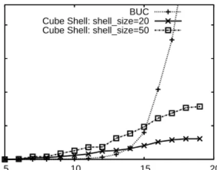
4.4 Performance Evaluations . . . 59
4.4.1 Shell Construction Efficiency . . . 60
4.4.2 Query Effectiveness . . . 61
Chapter 5 Moving Object Outliers . . . 68
5.1 Key Insights . . . 70
5.1.1 Motif-based Feature Space . . . 70
5.1.2 Multi-Resolution Feature Hierarchies . . . 72
5.2 Framework . . . 72 5.2.1 Motif Extractor . . . 73 5.2.2 Feature Generator . . . 75 5.2.3 Classification . . . 80 5.3 Experiments . . . 83 5.3.1 Real Data . . . 84 5.3.2 Synthetic Data . . . 86
Chapter 6 Subspace Outliers in Multidimensional Data . . . 93
6.1 Problem Definition . . . 94
6.1.1 Preliminaries . . . 94
6.1.2 The Anomaly Search Problem . . . 96
6.1.3 Ranking Anomalies in Data Cube . . . 97
6.2 Mining Top-K Anomalies in Data Cubes . . . 98
6.2.1 Retrieving σp(R) . . . 99
6.2.2 Selecting Candidate Subspaces . . . 100
6.2.3 Discovering Top-K Anomaly Cells . . . 104
6.2.4 Iterative Search . . . 104
6.3 Experiments . . . 105
6.3.1 Real World Data . . . 105
6.3.2 Synthetic Data . . . 108
Chapter 7 Temporal Traffic Outliers . . . 110
7.1 Road Segment Representation . . . 112
7.1.1 Input Data . . . 112
7.1.2 Feature Space . . . 113
7.2.1 Temporal Neighborhood Vector . . . 116
7.2.2 Temporal Vector Update Rules . . . 118
7.2.3 Temporal Outlier Scoring . . . 121
7.3 The TODFramework . . . 122
7.3.1 Complexity . . . 123
7.3.2 Setting Parameters . . . 123
7.3.3 Other Applications . . . 124
7.4 Experiments . . . 126
7.4.1 Outliers . . . 126
7.4.2 Na¨ıve Outlier Detection . . . 128
7.4.3 Efficiency . . . 129
Chapter 8 Conclusion . . . 132
References . . . 135
List of Tables
4.1 Two models of OLAP application . . . 38
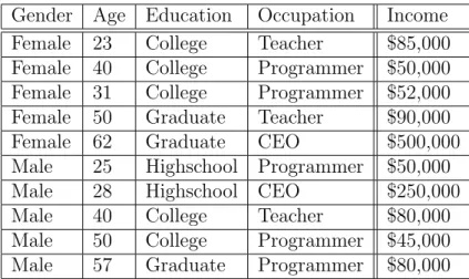
4.2 Sample survey data . . . 39
4.3 Query expansion experimental results . . . 67
6.1 Input market segment data . . . 95
6.2 Time Anomaly Matrix . . . 101
6.3 Attribute value AL scores . . . 103
6.4 Run times of trend anomaly query with low dimensional data (10≤ |R| ≤11) 106 6.5 Magnitude anomaly query run times . . . 106
7.1 Sample Feature Space . . . 114
7.2 Edge Similarity Values for Day 1 . . . 117
7.3 Day 1–3 Temporal Neighborhood Vectors . . . 120
List of Figures
1.1 Thesis Framework . . . 4
3.1 Snapshot of San Francisco Bay Area traffic . . . 15
3.2 Spectrum view of FlowScan and alternative methods . . . 17
3.3 Splitting hot routes: A→B →C and A→B →D . . . 19
3.4 Overlapping hot routes: A→B and B →C . . . 20
3.5 Slack within a hot route: A→B . . . 20
3.6 1-neighborhood of r. . . 22
3.7 Two sides of the same street . . . 22
3.8 Route traffic density-reachable . . . 24
3.9 Indexing structures of FlowScan . . . 28
3.10 Hot routes in San Francisco data map . . . 31
3.11 Hot routes in San Joaquin data map . . . 32
3.12 Splitting hot routes . . . 34
3.13 Overlapping hot routes . . . 35
3.14 Efficiency with respect to number of objects . . . 35
3.15 Disk I/O improvement of clustered index on Edge Table . . . 36
4.1 Cuboid lattice . . . 41
4.2 Query expansion within sampling cube . . . 46
4.3 Sampling Cube Shell . . . 52
4.4 Sampling cube shell construction example . . . 57
4.5 (Age, Occupation)query . . . 59
4.6 Materialization time vs. dimensionality . . . 61
4.7 Materialization time vs. number of tuples . . . 61
4.8 Query accuracy vs.shell size for average household income dataset . . . 64
4.9 Query accuracy vs. query dimensionality for average household income dataset 65 5.1 Motif representation . . . 71
5.2 ROAMFramework . . . 73
5.3 Two objects moving with the same trajectory. . . 75
5.4 Two sample motif-attribute hierarchies . . . 79 5.5 Path of ship Point Sur from 16:00 to 24:00 on 8/23/00 starting at point (0,0). 84
5.6 Extracted motifs from MBARI data. . . 85
5.7 Effect ofω on classification accuracy. . . 85
5.8 Effect of number of motifs on classification accuracy. . . 86
5.9 GSTDN2000B200M30: Accuracy with respect to difference in variance. . . 87
5.10 N4kB200A3S5.0L20: Accuracy with respect to number of motifs. . . 88
5.11 N4kB200A3S5.0L20: Accuracy with respect to length of motif-trajectories. . 89
5.12 N5kB100M20A3L20: Accuracy with respect to standard deviation. . . 89
5.13 N500B100M20A3S25L20: Accuracy with respect to β. . . 90
5.14 N15kB500A3S25L20: Accuracy with respect to number of motifs. . . 90
5.15 GSTD: B200M20: Efficiency with respect to number of trajectories. . . 91
5.16 N20000B1000M20A3S10.0: Efficiency with respect to length of motif-trajectories. 91 5.17 GSTD: N2000B100M10: Efficiency with respect to length of trajectories. . . 91
6.1 Cuboid lattice . . . 95
6.2 SUITS Framework . . . 99
6.3 Running time vs. number of dimensions . . . 107
6.4 Running time vs. number of tuples . . . 108
6.5 Running time vs. number of dimensions . . . 109
6.6 Running time vs. length of time series . . . 109
7.1 Historical Speed on Road Segment X . . . 111
7.2 Historical Speed on Many Road Segments . . . 111
7.3 Stability of Average Daily Speed and Load . . . 114
7.4 Speed and Load Neighborhood Stability . . . 116
7.5 Similarity-based Reward/Penalty tovi,j . . . 119
7.6 TODData Flow . . . 123
7.7 Temporal Similarity . . . 125
7.8 Speed Outlier (14th St.) . . . 127
7.9 Speed Outlier (Webster Ave.) . . . 127
7.10 Load Outlier . . . 127
7.11 Load Outlier . . . 128
7.12 Non-Outlier . . . 128
7.13 Average Speeds of I-880 . . . 130
7.14 Average Speeds of San Jose Ave. . . 131
7.15 Efficiency vs. Number of Days . . . 131
7.16 Efficiency vs. Neighborhood Radius . . . 131
Chapter 1
Introduction
In recent years, analysis of moving object data [24] has emerged as a hot topic both academ-ically and practacadem-ically. On a macro level, trajectories of airplanes or ships are being tracked constantly by either the company who runs them or the government. On a micro level, GPS devices embedded in vehicles or RFID sensors on the streets can track a vehicle as it moves throughout the city traffic grid. GPS devices in cellphones can even track an individual person as he/she walks around the city. There are many useful applications with such data. For instance, the OnStar system in General Motors vehicles notifies police of the vehicle’s GPS location when a crash is detected. Google Ride Finder provides real-time location of taxi cabs in many major cities through GPS devices installed in the cars. E-ZPass sensors (using RFID technology) automatically pay tolls so traffic is not disturbed. GPS navigation systems offer driving directions in real-time. Several cellphone services provide GPS tracking of children for parents or just tracking of nearby friends. On a more aggregate level, average speeds or traffic density is used to update driving time estimates in real-time or warn police of potential problem areas.
With such data and immediate applications, there are many exciting opportunities in research. Some basic ones include index and query. They are very important and funda-mental questions to tackle. But in addition to the basic real-world applications of simply asking “Where is this object?” or “Where has this object been?”, there are many higher level questions one could ask for moving objects data. Example 1 shows one particular problem which is of great interest in homeland security and surveillance.
Example 1 At any one time, there are approximately 160,000 vessels traveling in the United States’ waters. They include military cruisers, private yachts, commercial liners, and so on. The US Navy and Coast Guard are constantly on the lookout for suspicious behaviors. The traditional model of surveillance has been manual inspection of RADAR. However, as the number of vessels increases and the cost of manpower increases, it is becoming unrealistic to manually examine each of these vessels and identify the suspicious ones. Thus, it is highly desirable to create automated tools that can evaluate the behavior of all maritime vessels and develop situational awareness on the abnormal ones.
Example 1 shows an example of anomaly detection in the military. More close to home are surveillance applications. Recently in Chicago, millions of dollars have been invested to install hundreds of cameras at street corners. Though they are being used to many different purposes, one is to track the movement of vehicles. By reading the license plate number, the cameras can track a vehicle as it moves throughout the city. This tracking can be used for criminal investigations and also anti-terrorism purposes. One simple example the city gave was that if a vehicle is observed at a particularly sensitive street corners three times within a short period of time, the system would automatically raise an alarm. This is a rather simple rule; one could imagine a much more sophisticated system at work.
On a less security-focused front, imagine the following application of moving object tech-nology.
Example 2 Many modern-day cellphones are equipped with GPS technology that can pin-point the user anywhere on Earth. Even without GPS, one could use triangulation of the cellphone towers to narrow down the location of the user to within a few city blocks. This effectively says that all cellphone users’ locations can be tracked. For the purpose of studying and predicting consumer behavior, this is a great source of data. By knowing the location of people in various stores and malls across the city, one can very accurately measure and predict the sales of goods at all types of stores.
The above example shows the great power of tracking moving objects. If one can predict the sales of goods at a chain of stores, one can fairly accurately predict the quarterly sales number of the company. This leads to better prediction of stock prices and much better “playing” of the stock market than conventional analysts.
Similarly, but on a much more micro level, one can imagine tracking customers inside a single store. RFID technology can be installed on shopping carts and baskets and be used to track customers as they wander the store. Such trajectories can be used to better model consumer behavior and possibly better store layouts to maximize revenue.
The above two examples give relatively high level problems in the moving object domain. Problems of this type are the focus of this thesis. Instead of asking basic questions such as “Where is object X?”, we ask higher level and more aggregated questions such as “What are the behaviors of objects of type X?” In the context of previous examples, typeX could be “suspicious vehicles” or “potential buyers.” The much more loaded term in that question is “behaviors.” Behavior can be defined in an infinite number of ways. In the context of spatiotemporal data, it could be a movement pattern in space (e.g., right turn), an attribute of movement (e.g., speed), or an attribute in time (e.g., 10:00am). Such behaviors or patterns are easy to describe in human terms but to have an algorithm extract them automatically is another question. Furthermore, implied in our question is the term “interesting” in front of “behaviors.” Since the goal is to learn more about objects of typeX, uninteresting behaviors are fairly useless. For examples, knowing that many vehicles drive on the highway is common knowledge and does not add much to the study. But to define interestingness is a tricky issue. Is it something that is frequent? Does it have to be unique to type X? Depending on the application, different interestingness measures can be employed.
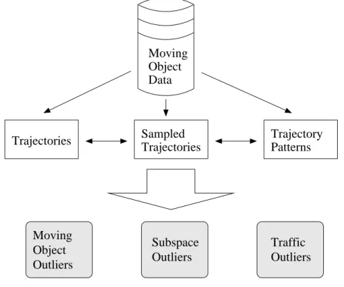
In this thesis, we are looking for patterns in moving object trajectories for the purpose of extracting high level knowledge. To this end, we present several studies that fit into an overall framework. Figure 1.1 shows the flow of data in the framework. At the top is the
original raw moving object data. The middle level serves as a pre-processing step which may clean the data in some form. The bottom layer is the analysis layer which then extracts the final patterns. Moving Object Data Sampled Trajectories Trajectories Trajectory Patterns Subspace Outliers Moving Object Outliers Traffic Outliers
Figure 1.1: Thesis Framework
The rest of this thesis will describe the modules in Figure 1.1 in detail. First, to allow all our analysis studies to operate on a higher semantic level, Chapter 3 studies the extraction of hot routes in traffic data [51]. This step lets algorithms operate on a more aggregated in-formation rather than individual road segments or trajectory pieces. Next, in many studies, only a sample of the population is available for study. How to deal with the lack of data in a multidimensional space [52] is addressed in Chapter 4. The next three chapters corre-spond to the three outlier detection modules in Figure 1.1. Moving from left to right, we first present ROAM[50], which detects moving object outliers in a free-moving environment and will be discussed in Chapter 5. Next, we consider outliers in arbitrary subspaces of a multidimensional space. Analysis of moving object data is often multidimensional. That is,
there are multiple dimensions of attributes attached to the data and one can analyze them from arbitrary angles. This introduces outliers in multidimensional space [47], which is the subject of our study in Chapter 6. Lastly, we present TOD [53], which detects temporal outliers in the traffic of a road network and will be discussed in detail in Chapter 7. We conclude our studies and discuss some future work in Chapter 8.
Chapter 2
Related Work
Compared to other more mature fields, research with moving objects is still in its infancy. Much of the work is still focused on relatively fundamental, yet very important, questions such as indexing and query processing. In this section, we will review the current research in all related areas and also how they relate to our own planned work. For completeness, we will include work from the field of spatiotemporal research. Because it considers all spatial objects (not just moving ones), it can be viewed as a superset of moving objects research.
2.1
Indexing and Query Processing
A basic task people like to perform on data is indexing. Given a large amount of data, the most basic question to ask is “What is in it?” For spatiotemporal data, it is more like “Where is it?” or “Where was it at this particular time?” Questions such as these can only be answered efficiently if there is a proper index on the data.
In discussing various types of indices and query processing, we are going to divide them into two main groups. The first are stationary objects (either having size or not) and the second aremoving objects. While stationary objects may seem unrelated to our work, many of the techniques in that field are quite useful. Further, because our work involves spatiotem-poral data in general, it will often require analysis on stationary spatial objects. Thus, we will discuss both types of data in the following two sections.
2.1.1
Stationary Spatial Data
The R-tree index [25] was invented for the purpose of accessing points in multi-dimensional space. Though it can handle all types of spatial data whether the points have size or not. Based on the B-tree, it uses the concept of minimum bounding rectangles. Each non-leaf node in the tree is a bounding rectangle that spatially contains all nodes (i.e., objects) in its subtree. To search for an object, one would start at the root node (the bounding rectangle that contains all objects) and progressively drill down to smaller rectangles until the query is satisfied.
Many extensions of the original R-tree have been proposed; some can handle moving objects as well. They include the R*-tree [6], R+-tree [70], X-tree [8], Hilbert R-tree [34], CR-tree [37], CT-R-CR-tree [16], CR*-CR-tree, Hilbert CR-CR-tree, and more. A performance comparison can be found at [29].
In relation to our work of data mining in moving objects, such indexing algorithms can be very helpful. In some of our work [51], spatial queries are needed to find stationary objects (namely street intersections) near a particular location. Having a faster index would only make our algorithm more efficient.
In additional to basic window queries, algorithms [67, 72, 15] have also been proposed to efficiently process nearest-neighbor queries. These are well-known problems in traditional database research that has been ported to spatiotemporal research. But, the nature of spatiotemporal data has also introduced a new kind of query, one where the query (be it a region or a point) moves. A natural real-world application is to find the nearest restaurant as one moves through a city.
A na¨ıve approach to this problem is to continuously apply the traditional stationary algo-rithms repeatedly as the query moves. This would surely work but could be very inefficient. For instance, if the query moves very little, the results might not change at all. By knowing this, one could save an entire query.
Several algorithms [76, 91] have been proposed to tackle this problem. In one of the earlier work [76], it was proposed to process the query by issuing the entire query segment (i.e., the object’s trajectory) to an R-tree instead of point-by-point. This reduces many redundant queries. The authors also introduce heuristics for pruning parts of the R-tree by calculating distances between nodes and the query segment. In [91], the concept of a valid region for the query location is introduced. As long as the query object remains in the valid region, there is no need to re-evaluate the query (either nearest-neighbor or window). By being aware, this greatly reduces the number of evaluations on the query.
And finally, related to index and query is data warehousing [59, 62, 46, 74, 75]. In-stead of focusing on individual object’s locations, queries seek aggregate information on historical data. Other studies have focused on approximate aggregate queries [73]. In it, multi-dimensional histograms are used to approximate the aggregation queries.
2.1.2
Moving Object Data
The previous section discussed indexing structures and queries for spatial objects that did not move. The more relevant scenario to our work is when do they move. One of the first work to touch on this topic was the TPR-tree [69], which is atime-parametrized R-tree. Like the R-tree, non-leaf nodes in the tree are bounding rectangles that contain all points in the subtree. But additionally, each rectangle also has a velocity vector. Then, depending on the setting of the time parameter, one could calculate the new position of the rectangle for some time in the future. By doing the same calculation for a possibly moving query rectangle, one can then check if the query rectangle and any object rectangle will intersect at any time. This framework has been extended [77, 68] and used [7, 17, 64, 43].
A different class of solutions for the same problem uses the idea of dual spaces. Trajec-tories are converted into points in a different space and indexed and queried accordingly. Some examples of this idea include algorithms which convert trajectories to points in higher
dimensional spaces [39, 1, 61, 40]. One particular example is STRIPES [61]. Instead of using the R-tree and modeling linear trajectories, entire trajectories are transformed to points in a higher dimensional space. Specifically, given a moving object in d-dimensional space, the maximum velocity vector (d-dimensional vector) combined with reference position vector (d-dimensional vector) forms a new 2d-dimensional point. These points are then stored in a multi-dimensional quadtree. And finally, there is work that transforms trajectories to points in a lower dimensional space. The Bx-tree [32, 55] and Bdual-tree [86] are examples in which
the moving objects are converted to 1-dimensional values using space-filling curves and then stored in a B+-tree.
With continuously moving objects, many traditional queries can be converted to “con-tinuous” as well. More specifically, instead of just executing the query once and getting the results, the query executes continuously and the results are updated as the objects moves. First, consider the case where the movements of the objects are known a priori. Nearest neighbor queries on them have been studied in [30, 31, 66]. In general, one might not know any information before evaluating the query. Some studies [32, 57, 58, 89, 83] basically re-evaluate the query periodically using the new moved data. A recent work [28] also works on this problem without making any assumptions. It extends the idea of valid regions [91] to both the query and the objects themselves. One of the goals of the framework is reduce the amount of communication between objects (both the querying object and the queried objects) and the central database, which keeps track of queries and moving objects. In this framework, each moving object is aware of a safe region. As long as the object moves inside this region, it will not affect the result of the queries that the central database is currently handling. But, if the object moves outside the region, it will update the central server of its new location and the central database will take care of updating query results and also new safe regions. By doing this, not only is the number of query calculations reduced, the amount of communication between the object and the central database is also reduced.
One particular type of moving object data that is of interest to us is moving objects on
road networks or constrained networks. New techniques [63, 20, 4, 13] are needed to take advantage of the constraints. In [63], a dimensionality reduction technique is used to reduce the 3D problem (i.e., 2D spatial plus time) into lower-dimensional problems. The FNR-tree [20] also uses a dimensionality reduction technique. A 2D R-tree is used to index all the edges in the road network. Then, the objects within each object are further indexed by a different 1D R-tree. In other words, there is a main 2D R-tree for indexing the network’s edges and many different 1D R-trees in the leaves of the main tree for indexing objects. Experimental results show that this indexing scheme is more efficient in terms of space utilization and search speed than a 3D R-tree. More recently, the idea of an adaptive unit (AU) was introduced in [13]. A single AU is similar to a MBR in the context of the TPR-tree [69]. However, in the traditional TPR-tree, objects with very different movement patterns may exist in a single MBR. If they happen to move in opposite directions, it will expand the MBR very quickly and require many updates. In contrast, an AU will contain only objects with similar movement patterns; it can be viewed as a moving object cluster. The AUs are then indexed by an R-tree, similar to the original TPR-tree. The authors show empirically that the AU-index is much more efficient with respect to updates than the TPR-tree.
2.2
Data Mining
Data mining in the spatiotemporal domain has also received some attention. One of the most immediate extensions from traditional data mining is the discover of frequent patterns. One of such studies finds frequent sequences in spatiotemporal data [79]. In their setting, data consists of sequences of events at spatial locations. For example, locations could be cities in the United States, and the sequential data could be temperature recordings. The goal is then to find frequent sequential patterns in the data. The authors tackle this problem in a
two-step process. First, a depth-first mining algorithm is proposed to discover sequential patterns at individual locations. The algorithm uses the enumeration lattice structure proposed in SPADE to efficiently discover maximal frequent sequences. Then, to incorporate the spatial aspect of the data, the algorithm examines the hierarchical nature of the locations. In the United States for example, one could roll the locations up to the county or state level. This hierarchy information is pushed down to the mining algorithm and an apriori-like property is found to aid in the pruning of the algorithm.
Another popular problem with spatiotemporal data is co-location mining. This is very similar to the traditional association mining. The biggest difference is that the predicates in the pattern can be spatial or temporal or both. For example, in traditional association mining, itemset A might be found to be frequently associated with B in the transaction database. In co-location mining, the constraint of A being near B (where A and B are spa-tiotemporal events) could be enforced. This neighborhood constraint add to the complexities of the traditional mining algorithm. Some studies [41, 71, 88] have modified traditional asso-ciation mining algorithms to incorporate the spatiotemporal information. For instance, the apriori algorithm has been extended [71, 88] to join smaller co-location patterns together. [88] performs a more complicated process by looking additionally at partial joins. [93] is a recent work that quickly finds co-location patterns by using multiway joins.
A problem related to nearest-neighbor queries is the computation of influential sites [81, 19]. The influence of a particular site is measured by how many other sites has it as its nearest neighbor. This has also been called the reverse nearest-neighbor problem. Though the concept of the problem is not unique to spatial data, the solution uses spatial solutions such as the R-tree. Related to influential queries are preference queries [87]. A preference query is like a regular query except that it considers extra features to the data. For instance, a query asking for a ranked list of houses in a neighborhood might uses a combinations of features (i.e., size, price, school quality, etc) in its ranking. This combination of spatial
information and other multi-dimensional features pose new challenges.
2.3
Clustering
Clustering of moving objects and trajectories is a useful problem in many contexts. Though very similar in goal, these two problems have a subtle difference. In moving object clustering, it is implied that the objects within a single cluster move with the same or similar trajectory
together. That is, they travel in a tight group. In trajectory clustering, only the final resultant trajectory is considered. One could say that the temporal component is ignored. Objects can move in arbitrary speeds or times, but as long as their final trajectories are similar, they will be clustered together. Some examples of moving object clustering include [36, 21, 11, 33]. In [33], objects are grouped using a traditional clustering algorithm at each time snapshot and then linked together over time to form moving clusters. The assumption is that clusters will be stable across short time periods.
Trajectory clustering has also produced some interesting results [90, 12, 44]. In one such work [12], trajectories are converted to line segments and a similarity function is defined between line segments. This similarity function is then used to mine for sequences of line segments, which grows to the eventual pattern. A similar idea is employed in another work [44]. Though the goal in that work is slightly different: trajectory clustering vs. pattern discovering, the end result is quite similar. One could view the clusters as being the patterns. In [44], a minimum description length approach is taken to describe a trajectory as a sequence of lines. The lines are then fed into a density-based clustering algorithm to produce the final clusters. The similarity function used in clustering is like the one in [12] where the difference in angle and length factor into the final measure. Similarity functions between line segments or whole trajectories have also been explored in traditional similarity search [80, 14]. More recently, another work [22] attempted to solve the problem of discovering trajectory patterns.
In contrast to previous work, this one is more focused on higher level concepts. For instance, instead of discovering a pattern involving a specific spatial location, a general location (e.g., airport) is found. Such general locations are called Regions-of-Interest or RoI’s. Then, frequent movement patterns between the RoI’s are discovered.
Finally, there is the area of trajectory modeling [54, 42]. Here, the goal is very different. Instead of just producing frequent patterns, an entire model is constructed that describes how the object will move under various situations. A Markov model is typically used for such problems. Also, each model is typically used to describe just a single object. Multiple objects with slightly varying transition probabilities can not be efficiently captured within a single model. This makes it unsuitable for hundreds or thousands of objects. Lastly, it is not clear that moving objects satisfy the Markovian property. Without it, the models will not be very effective.
Chapter 3
Hot Route Detection
As previously mentioned, clustering is a very attractive problem in moving objects research. It is a very natural question to ask about moving objects and algorithms can leverage much of the current work in traditional clustering. A related question is to ask what are the hot routes or the general traffic flow pattern in a city road network. The set of hot routes offers direct insight into the city’s traffic patterns. City officials can use them to improve traffic flow. Store owners and advertisers can use them to better position their properties. Police officials can use them to maximize patrol coverage.
This is a challenging problem due to the complex nature of the data. If objects traveled in organized clusters, it would be straightforward to use a clustering algorithm to find the hot routes. But, in the real world, objects move in unpredictable ways. Variations in speed, time, route, and other factors cause them to travel in rather fleeting “clusters.” These properties make the problem difficult for a naive approach. To this end, we propose a new density-based algorithm namedFlowScan[51]. Instead of clustering the moving objects, road segments are clustered based on the density of common traffic they share. We implemented
FlowScan and tested it under various conditions. Our experiments show that the system is both efficient and effective at discovering hot routes.
Example 3 Figure 3.1(a) shows live traffic data1 in the San Francisco Bay Area on a
week-day at approximately 7:30am local time. Different colors show different levels of congestion (e.g., red/dark is heavy congestion). 511.org in the Bay Area gathers such data in
real-1
time from RFID transponders located inside vehicles2. A likely hot route in Figure 3.1(a)
is A → B (i.e., highway CA-101). A is near the San Francisco International Airport. B
is near the San Mateo Bridge. Figure 3.1(b) shows a closeup view of location B. Three additional locations x, y, and z are shown. Without actually observing the flow of traffic, it is unclear whether y →x is a hot route, or y → z, or x → z. FlowScan aims to solve this
problem.
(a) (b)
Figure 3.1: Snapshot of San Francisco Bay Area traffic
At first glance, this may seem like an easy problem. A quick look at Figure 3.1(a) shows the high traffic roads in red. With some domain knowledge, we know that San Francisco, Oakland, and other densely populated regions are likely to be sources and destinations of traffic since many people live and work there. However, such domain knowledge is not always available. Additionally, real world traffic is a verycomplex data source. Objects do not travel in organized clusters. Two objects traveling from the same place to another place may take just slightly different routes at slightly different speeds and times. Random traffic conditions, such as a traffic accident or a traffic light, can cause even more deviations. Furthermore, hot routes do not have to be disjoint. Highways or major roads are popular pathways and
2
several hot routes can share them. As a result, the mining algorithm must be robust to the variations within a hot route and amongst a set of hot routes.
We now state our problem as follows: Given a set of moving object trajectories in a road network, find the set of hot routes. A road network is represented by a graph G(V, E). E
is the set of directed edges, where each one represents the smallest unit of road segment.
V is the set of vertices, where each one represents either a street intersection or important landmark. T is the set of trajectories, and each trajectory consists of an ID (tid) and a sequence of edges that it traveled through: (tid,he1, . . . , eki), where ei ∈ E. Objects can
only move onE and must travel the entirety of an edge. T is assumed to be collected from a similar time window; otherwise, different time windows might blur meaningful hot routes. Informally, ahot route is a general path in the road network which contains heavy traffic. It represents a general flow of the objects in the network. Formally, it is a sequence of edges inG. The edges need not to be adjacent in G, but they should be near each other. Further, a sequence of edges in a hot route should share a high amount of traffic between them.
3.1
Solution Overview
FlowScan extracts hot routes using the density of traffic on edges and sequences of edges. Intuitively, an edge with heavy traffic is potentially a part of a hot route. Edges with little or no traffic can be ignored. Also, two near-by edges that share a high amount of traffic between them are likely to be a part of the same hot route. This implies that the objects traveled from one edge to the other in a sequence. And lastly, a chain of such edges is likely to be a hot route.
We also list some possible alternative methods from related fields.
Alternative Method 1: Moving object clustering [21] discovers groups of objects that move together. The trajectory of each cluster can be marked as a hot route. We call this
class of approachesAltMoving.
Alternative Method 2: Simple graph linkage is another possible approach. One could gather all the edges in G with heavy traffic and connect them via their graph connectivity. Then, each connected component is marked as a hot route. We call this class of approaches
AltGraph.
Alternative Method 3: Trajectory clustering [44] discovers groups of similar sub-trajectories from the whole trajectories of moving objects. Each resultant cluster is marked as a hot route. We call this class of approaches AltTrajectory.
FlowScan and the three alternative methods offer very different approaches to the same data. One could view them in a spectrum. At one end of the spectrum are AltMoving and
AltTrajectory where attention is paid to the individual objects. This is helpful in problems where the goal is to identify behaviors of individuals. At the other end of the spectrum is AltGraph where attention is paid to the aggregate. That is, objects’ trajectories are aggregated into summaries and analysis is performed on the summary. This is helpful in problems where the goal is to learn very general information about the data. FlowScan can be viewed as an intermediate between these two extremes. The behaviors of the individuals (specifically, the common traffic between sequences of edges) are retained and affect high-level analysis about aggregate behavior.
Aggregate Analysis Individual Analysis FlowScan AltMoving/AltTrajectory AltGraph
3.2
Traffic Behavior in Road Networks
In this section, we list some common real world traffic behaviors and examine how FlowScan
and the alternative approaches can handle them.
3.2.1
Traffic Complexity
A major characteristic of real world traffic is the amount of complexity. Instead of neat clusters, objects travel with different speeds and times even when they are on the same route. For example, in a residential neighborhood, many people leave for work in the morning and travel to the business district using approximately the same route. However, it is very unlikely that a group will leave at the same time and also travel together all the way to their destination. Various events (e.g., traffic light) can easily split them up.
Algorithms in the AltMovingclass will not work very well with such complex data. Clus-ters in the technical sense only last for a short period of time or short distance. The same is true for AltTrajectory if speed/time is encoded into the trajectories. These algorithms lack
aggregate analysis and as a result, they are likely to find too many short clusters and miss the overall flow. FlowScan connects road segments by the amount of traffic they share. So even if the objects change slightly or if the objects do not travel in compact groups, the amount of common traffic between consecutive edges in a hot route will still be high.
3.2.2
Splitting/Joining Hot Routes
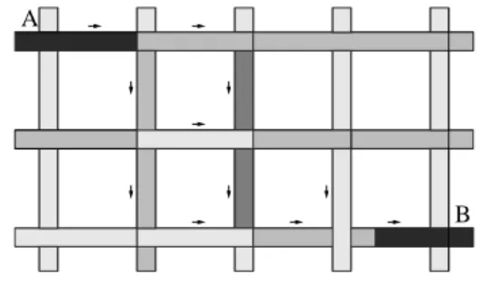
Figure 3.3 shows a sample city traffic grid. The shade on each road segment indicates the amount of traffic on it; the darker the shade, the heavier the traffic. Suppose the two correct hot routes areA→B →C and A→B →D. Figure 3.3 shows a splitting of traffic at node
B: some objects which moved from A to B go to C while others go to D. There are also other objects which move fromC toDand vice-versa. This situation is very common in real
world traffic. B could be the location in Chicago where I-90/94 splits into I-90 and I-94.
A B
C
D
Figure 3.3: Splitting hot routes: A→B →C and A→B →D
WithAltGraph, since all edges fromAtoCandDare connected, they would be incorrectly identified as a single big hot route. Notice that there is no individual analysis in AltGraph. With AltTrajectory, A → B and B → C will not be joined together because the physical similarity between them is low (i.e., hard left turn). Likewise for A → B → D. This flaw exists for the joining of traffic as well. In other words, if the arrows in Figure 3.3 were reversed, it would illustrate the problem of two hot routes joining atB.
In FlowScan, edges B → C and B → D will not be connected directly because they do not share any traffic. This is because physically, objects have to choose between the two edges and cannot travel on both. Further, A → B will be connected to both B → C and
B →D because it shares traffic with both.
3.2.3
Overlapping Hot Routes
In addition to splits or joins, two hot routes may overlap each other. Figure 3.4 shows an example with two distinct hot routes: A →B and B →C. Situations like this are common. Suppose B is a parking garage used by nearby residents during the night and incoming workers during the day. In the morning, residents drive out of the parking garage (B →C) and other people arrive from various locations to park (A→B).
Consider howAltGraphwill handle this situation. SinceA→B andB →Care connected in G at node B, the two hot routes will be joined together incorrectly. This is due to the
A B C
Figure 3.4: Overlapping hot routes: A→B and B →C
lack ofindividual analysison the edges during linking. The same happens withAltTrajectory, though for a different reason. A→B and B →C’s shapes are similar and will be clustered together. With FlowScan, consecutive edges within a hot route must share a minimum number of common objects. If such edges were parts of different hot routes, this condition will not be satisfied, and thus, a single erroneous hot route will not be formed.
3.2.4
Slack within Hot Routes
Figure 3.5 shows a hot route with some slight slack. A hot route exists from A to B in the grid. At the intermediate locations, objects are faced with different choices in order to reach
B. Suppose the choices are essentially equivalent in terms of distance and speed and that traffic is split equally between them.
B A
Figure 3.5: Slack within a hot route: A→B
Consider how AltMoving will handle this deviation. Suppose the distance between the equivalent paths is larger than the maximum intra-cluster distance. This will cause the cluster atAto break into several smaller clusters when it reachesB. Next, considerAltGraph. Suppose the partitioning of traffic reduced the density on the intermediate edges to be below the “heavy” threshold. This would break the graph connectivity condition and miss the hot
route from A to B. A similar error could occur with AltTrajectory if the traffic becomes too diluted between A and B or if the shapes become too dissimilar. With FlowScan, edge connectivity in G is not a required condition. Edges are connected in the hot route if they share common traffic and if they are near each other. Here, as long as A is within a given distance from B, the hot route will remain intact.
3.3
Density-based Hot Route Extraction
In this section, we will give formal definitions of FlowScan, which uses traffic density infor-mation in road networks to discover hot routes.
3.3.1
Traffic-Density Reachability
Definition 1 (Edge Start/End) Given a directed edge r, let the start(r) be the starting vertex of the edge and end(r) be the ending vertex.
Definition 2 (ForwardNumHops) Given edges r and s, the number of forward hops be-tweenrandsis the minimum number of edges betweenend(r)andend(s)inG. It is denoted
as F orwardN umHops(r, s).
Recall thatG is directed. This implies that an edge that is incident tostart(r) inG will not have aF orwardN umHops value of 0 unless it is also incident to end(r).
Definition 3 (Eps-neighborhood) TheEps-neighborhoodof an edger, denoted byNEps(r),
is defined by NEps(r) = {s∈E|F orwardN umHops(r, s)≤Eps} where Eps≥0.
The Eps-neighborhood of r contains all edges that are within Eps hops away from r, in the direction ofr. Semantically, this captures the flow of traffic and represents where objects are within Eps hops after they exit r. Figure 3.6 shows the 1-neighborhood of edge r.
Note that having the forward direction in theEps-neighborhood makes the relation non-symmetric. In Figure 3.6 for example, the two edges in the circle are in the 1-neighborhood of r, but r is not in the 1-neighborhood of either of them. In fact, the only time when the Eps-neighborhood relation is symmetric is when two edges form a cycle within themselves. This is usually rare in road networks with one exception, and that is when one considers two sides of the same street. Figure 3.7 shows an example. In it, r0 is in the 1-neighborhood of
r1 and vice-versa, because they form a cycle. This will happen for all two-way streets in the network. Though typically, an object will not travel on both sides of the same street within a trajectory. It could only happen with U-turns or if one end of the street is a dead end.
rr Figure 3.6: 1-neighborhood of r.
r
r
1 0Figure 3.7: Two sides of the same street
We did not choose a spatial distance function (e.g., Euclidean distance), because the number of hops better captures the notion of “nearness” in a transportation network. Con-sider a single road segment in the transportation network. If it were a highway, it might be a few kilometers long. But if it were a city block in downtown, it might be just a hundred meters. However, since an object has to travel the entirety of that edge, the two adjacent edges are the same “distance” apart no matter how long physically that intermediate edge is.
Definition 4 (Traffic) Let traffic(r) return the set of trajectories that contains edger. Re-call trajectories are identified by unique IDs.
Definition 5 (Directly traffic density-reachable) An edge s is directly traffic density-reachable from an edge r wrt two parameters, (1) Eps and (2) MinTraffic, if all of the following hold true.
1. s∈NEps(r)
2. |traffic(r)∩traffic(s)| ≥MinTraffic
Intuitively, the above criteria state that in order for an edge s to be directly traffic density-reachable from r, smust be near r, andtraf f ic(s) andtraf f ic(r) must share some non-trivial common traffic. The “nearness” between the two edges is controlled by the size of the Eps-neighborhood. This directly addresses the slack issues in Section 3.2.4. As long as the slack is not larger thanEps, two edges will stay directly connected via this definition. The second condition of two edges sharing traffic is intuitive. It is also at the core of
FlowScan. The flaw of methods in the AltGraph class is that aggregation on the edges has erased the identities of the objects. As a result, two edges with high traffic on them and near each other will look the same regardless if they actually share common traffic. By having the second condition rely on the common traffic, one can get a better idea of how objects actually move in the road network.
Directly traffic density-reachable is not symmetric for pairs of edges because the Eps-neighborhood is not symmetric. Though, for the same reasons that two edges might be in the Eps-neighborhood of each other, two edges could be directly traffic density-reachable from each other.
Definition 6 (Route traffic density-reachable) An edgesisroute traffic density-reachable
from an edge r wrt parameters Eps and MinTraffic if:
1. There is a chain of edges r1, r2, . . ., rn, r1 = r, rn = s, and ri is directly traffic
density-reachable from ri−1.
2. For every Eps consecutive edges (i.e., ri, ri+1, . . ., ri+Eps) in the chain, |traffic(ri)∩
Definition 6 is an extension of Definition 5. It states that two edges are route reachable if there is a chain of directly reachable edges in between and that if one were to slide a window across this chain, edges inside every window share common traffic. The sliding window directly address the overlapping behavior as described in Section 3.2.3. At the boundaries of two overlapping hot routes, the second condition will break down and thus break the overlapping hot routes into two. The Eps parameter is being reused here to control the width of a sliding window through the chain. The reuse is justified because their semantics are similar, but one could just as well use a separate parameter.
The reason for using a sliding window is based on our observation that a trajectory can contribute to only a portion of a hot route. This better matches real world hot route behavior. For example, a hot route exists from the suburb to downtown in the morning. Figure 3.8 shows an illustration. However, most people do not travel the entirety of the hot route. More often, they live and work somewhere in between the suburb and downtown. But in the aggregate, a hot route exists between the two locations.
Suburbs
Downtown
Figure 3.8: Route traffic density-reachable
3.3.2
Discovering Hot Routes
The hot route discovery process follows naturally from Definition 6. It is an iterative process. Roughly, one starts with a random edge, expands it to a hot route, and repeats until no more edges are left. The question is then with which edge(s) should each iteration begin. To this end, we introduce the concept of a hot route start, which is the first edge in a hot route. Intuitively, an edge is a hot route start if none of its preceding directly traffic
density-reachable neighbors are part of hot routes.
Definition 7 (Hot Route Start) An edge r is a hot route start wrt MinTraffic if the following condition is satisfied.
traffic(r)\ [ traffic(x) ≥MinTraffic
where {x|end(x) = start(r)∧ |traffic(x)| ≥MinTraffic}.
The question is whether all hot routes begin from a hot route start. The following lemma addresses this.
Lemma 1 (Hot Route Start) Hot routes must begin from a hot route start.
Proof: There are two ways for a hot route to begin on an edge r. The first way is when MinTraffic or more objects start their trajectory at r. In this case, none of these objects will appear in start(r)’s adjacent edges because they simply did not exist then. As a result, the set difference will return at least MinTraffic objects and thus marking r as a hot route start. The second way is when MinTraffic or more objects converge at r from other edges. The source of traffic on r is exactly the set of edges adjacent to start(r). Suppose one of these edges,x, contains more thanMinTraffic objects on it. In this case,xis part of another hot route, and the objects that moved fromx tor should not contribute tor. However, if it does not contain more than MinTraffic objects, it cannot be in a hot route and its objects are counted towardsr. If more than MinTraffic objects are counted towardsr, then it is the start of a hot route.
3.3.3
Algorithm
Definitions 6 and 7 form the foundation of the hot route discovery process. A simple approach could be to initialize a hot route to a hot route start and iteratively add all route traffic
density-reachable edges to it. By repeating this process for all hot route starts in the data, one can extract all the hot routes. The question is then how to efficiently find all route traffic density-reachable edges given an existing hot route. If new edges are added in no particular order, then one would have to search through all existing edges in the hot route at every iteration. This is very inefficient. Further, if the hot route splits, it could become tricky if it is in the middle.
To alleviate this problem, we restrict the growth of a hot route to be only at the last
edge. A hot route is a sequence of edges so the last edge is always defined. By growing the hot route at the end one edge at a time, only the Eps-neighborhood of the last edge needs to be extracted. This is much more efficient than extracting the Eps-neighborhoods of all edges in the hot route. This is still a complete search because all possible reachable edges are examined but just with some order. It is essentially a breadth-first search of the road network. Then for each neighboring edge, the route traffic density-reachability condition is checked against the last few edges of the hot route (i.e., window). If the condition is satisfied, the edge is appended to the hot route; otherwise, the edge is ignored.
Sometimes, the number of directly traffic density-reachable edges from the last edge in the hot route is larger than one. There are two causes for this. The first cause is multiple edges within one hot route. This can happen whenEps is larger than 0, and multiple edges of the hot route are in the Eps-neighborhood. This can be detected by checking to see if
the start()’s andend()’s match across edges. In this case, only the nearest edge is appended
to the hot route. The other edges will just be handled in the next iteration. The second cause is when a hot route splits. In this case, the current hot route is duplicated, and a different hot route is created for each split. The difference between these two cases can be detected by checking the directly traffic density-reachability condition between edges in the Eps-neighborhood.
the data. This is done by checking Definition 7 for every edge in G. This step has linear complexity because only individual edges with their Eps-neighborhoods are checked. Then, for every hot route start, the associated hot routes are extracted. Algorithm 1 shows a pseudo-code description.
Algorithm 1FlowScan
Input: Road network G, object trajectory data T, Eps, MinTraffic. Output: Hot routes R
1: Initialize R to{}
2: LetH be the set of hot route starts in G according toT 3: for every hot route start h inH do
4: r = new Hot Route initialized to hhi
5: Add Extend Hot Routes(r) to R 6: end for
7: Return R
Procedure Extend Hot Routes(hot router)
1: Letp be the last edge in r
2: LetQ be the set of directly traffic density-reachable neighbors ofp 3: if Q is non-empty then
4: for every split in Qdo
5: if route traffic density-reachable condition is satisfied then
6: Letr′ be a copy of r
7: Append split’s edges tor′ 8: Extend Hot Routes(r′)
9: end if
10: end for
11: else
12: Return r 13: end if
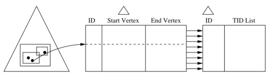
One point of concern is efficiency. Suppose the adjacency matrix or list of the road net-work fits inside main memory. Then, searching the graph is quite efficient. Retrieving the list of TID’s at each edge will require disk I/O but traversing the graph will not. However, suppose the adjacency matrix is too big to fit inside main memory. In this case, we in-troduce two additional indexing structures to help the search process. Figure 3.9 shows an
illustration.
Edge Table
ID Start Vertex End Vertex ID TID List
TID List Table Vertex Index Tree
Figure 3.9: Indexing structures of FlowScan
All vertices of the road network are stored in a 2D index,e.g., R-tree (Vertex Index Tree). All edges are stored on disk (Edge Table). Each edge record consists of the edge ID and its starting and ending vertices (each vertex is an (x, y) tuple). Using these two data structures, one can retrieve adjacent neighbors of an edge by querying the R-tree on the appropriate vertex and then retrieving the corresponding edges in the Edge Table. The R-tree is quite useful for finding adjacent neighbors of a specific edge since the coordinates of the adjacent neighbors tend to be close to that of the edge.
We note that the Edge Table may be accessed repeatedly to retrieve adjacent neighbors. This operation can be done more efficiently by exploiting locality. Specifically, if the physical locality of edges in the road network is preserved in the Edge Table, one can reduce the amount of disk I/Os. To this end, we create a clustering index on the Starting Vertex attribute of the Edge Table. Assuming that each value is 4 bytes, each edge record is then 20 bytes. Then, if a page is 4K, it will contain approximately 200 edges. The intuition is that these 200 edges will be physically close to each other in the road network. BecauseFlowScan
traverses through Eps-neighborhoods, it is highly likely that an edge and its neighbors will be stored on the same page in the Edge Table. In this case, disk I/O will be reduced because the page has already been fetched.
Lemma 2 (Completeness) The set of hot routes discovered by FlowScan is complete and
Proof: The above assertion is easy to see because the construction algorithm uses the definition word-for-word, specifically Definition 6, to build the hot routes. Thus, given a hot route start, the set of hot routes extending from it is guaranteed to be found. The question is more about if the set of hot route starts found is complete. Because every edge in a hot route must satisfy theMinTraffic condition, there must be a “first” in a sequence. The set of hot route starts is simply these “firsts.” Lastly, ordering is not a factor inFlowScan, because no marking or removal is done toG. Thus, it does not matter in which orderHis processed.
3.3.4
Determining Parameters
There are two input parameters to the FlowScan algorithm: Eps and MinTraffic. The first parameter,Eps, controls how laxFlowScancan be between directly reachable edges. A value of 0 is too strict since it enforces strict spatial connectivity. A small value in the range of 2–5 is usually reasonable. In a metropolitan area, this corresponds to 2–5 city blocks; and in a rural area, this corresponds to 2–5 highway exists.
As for MinTraffic, this is often application or traffic dependent. “Dense” traffic in a city of 50,000 people is very different from “dense” traffic in a city of 5,000,000 people. In cases where domain knowledge dictates a threshold, that value can be used. If no domain knowledge is available, one can rely on statistical data to set MinTraffic. It has been shown that traffic density (and many other behaviors in nature) usually obeys the power law. That is, the vast majority of road segments have a small amount of traffic, and a relative small number have extremely high density. One can plot a frequency histogram of the edges and either visually pick a frequency as MinTraffic or use the parameters of the exponential equation to set MinTraffic.
3.4
Experiments
To show the effectiveness and efficiency of FlowScan, we test it against various datasets.
FlowScan was implemented in C++ and all tests were performed on a Intel Core Duo 2 E6600 machine running Linux.
3.4.1
Data Generation
Due to the lack of real-world data, we used a network-based data generator provided by [10]3.
It uses a real-world city road network as the road network and generates moving objects on it. Objects are affected by the maximum speed on the road, the maximum capacity of the road, other objects on the road, routes, and other external factors.
The default generator provided generates essentially random traffic: an object’s starting and end locations are randomly chosen within the network. In order to generate some interesting patterns, we modified how the generator chooses starting and end locations. Within a city network, “neighborhoods” are generated. Each neighborhood is generated by picking a random node and then expanding by a preset radius (3–5 edges). Moving objects are then restricted to start and end in neighborhoods.
Hot routes form naturally because of the moving object’s preference for the quickest path. As a result, bigger roads (e.g., highways) are more likely to be chosen by the moving objects. However, if too many objects take a highway or a road, it will reach capacity and actually slow down. In such cases, objects will choose to re-route and possibly create secondary hot routes.
3
3.4.2
Extraction Quality
General Results
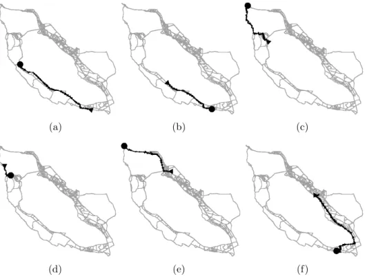
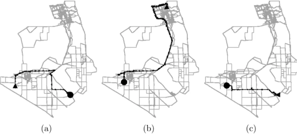
To check the effectiveness of FlowScan, we test it against a variety of settings. First, we present the results for two general cases. Figure 3.10 shows several routes extracted from 10,000 objects moving in the San Francisco bay area. 10 neighborhoods of radius 3 each were placed randomly in the map. Eps and MinTraffic were set to 2 and 300, respectively. Each hot route is drawn in black with an arrow indicating the start and a dot indicating the end. The gray lines in the figures indicate all traffic observed in the input data (not the entire city map).
(a) (b) (c)
(d) (e) (f)
Figure 3.10: Hot routes in San Francisco data map
Even though the neighborhoods were completely random, we get realistic hot routes in this experiment. The hot routes in Figure 3.10(a) and 3.10(b) are CA-101 connecting San Francisco and San Jose, a major highway in the area. Figures 3.10(c) and 3.10(d) correspond
to the Golden Gate Bridge connecting the city of San Francisco to the north. One of the random neighborhoods must have been across the bridge so objects had no choice but to use the bridge. Figure 3.10(e) shows a hot route connecting Oakland to that same neighborhood across the Richmond-San Rafael Bridge. Lastly, Figure 3.10(f) corresponds to a hot route connecting approximately Hayward to San Jose via I-880.
Next, Figures 3.11 shows three hot routes extracted from 5,000 objects moving in the San Joaquin network. Three neighborhoods were picked in this network, each with radius of 3. Eps and MinTraffic were set to 2 and 400, respectively. In Figures 3.11(a) and 3.11(b), the horizontal portions of the hot routes correspond to I-205. In Figure 3.11(b), the vertical portion corresponds to I-5. Both these roads are major interstate highways. The roads in Figure 3.11(c) are W. Linne Rd and Kason Rd. By looking at the city map, we observe that they make up the quickest route between the two neighborhoods.
(a) (b) (c)
Figure 3.11: Hot routes in San Joaquin data map
Splitting Hot Route Behavior
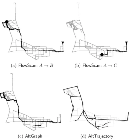
We also testedFlowScan with some specific traffic behaviors. First, we test the case of a hot route splitting into two. This data set is generated by setting the number of neighborhoods in a road network to three and fixing the start node to be in one of the three. Because start and destination neighborhoods cannot be the same, this forces the objects (1000 of them) to
travel to one of two destinations. And because the objects like to travel on big roads (due to speed preference), they will usually leave the starting neighborhood using the same route regardless of the final destination and split sometime later.
Figures 3.12(a) and 3.12(b) shows the two hot routes extracted from the data. Both hot routes start at the green arrow at the lower right, move to the middle, and the split according to their final destinations. In Figure 3.12(c), the result from anAltGraphalgorithm is shown. All edges that exceed theMinTrafficthreshold (100) are connected if they are adjacent in the road network. Obviously, the two hot routes are connected together because the underlying objects are not considered. Figure 3.12(d) shows the result from a AltTrajectory algorithm [44]. In it, 14 clusters were found. Because shape is a major factor in trajectory clustering, the routes were broken into different clusters. The split is “detected” simply due to the hard left-turn shape, but the routes are not intact. One could post-process the results and merge near-by clusters, but this could run into the same problems as AltGraph since individual trajectories are ignored.
Overlapping Hot Route Behavior
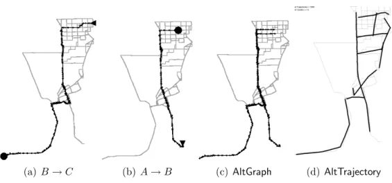
Next, we test the case of two hot routes overlapping. That is, one starts at the same place as where the other one ends. To generate this data set, we also set the number of neighborhoods to three. Let them be known as A, B, and C. Then, for half of the objects, their paths are
A →B; and for the other half, their paths are B →C. We set the radius of neighborhood
B to 0 to ensure that the two hot routes overlap.
Figure 3.13 shows the results of this test. As the graphs show, two hot routes were extracted. Figure 3.13(c) shows a result with anAltGraph algorithm. AlthoughB →C (not shown) is correctly extracted in that algorithm,A→Bis not. It is incorrectly linked together with B → C and erroneously forms A → B → C. This is because individual identities are not considered in the algorithm. Figure 3.13(d) shows the result ofAltTrajectory. 13 clusters
(a) FlowScan:A→B (b)FlowScan:A→C
(c) AltGraph (d)AltTrajectory
Figure 3.12: Splitting hot routes
were discovered. Again, the routes are not intact. But more seriously, the trajectories near
B are clustered into a single cluster because their shapes are similar.
3.4.3
Efficiency
Finally, we test the efficiency of FlowScan with respect to the number of objects. Figure 3.14 shows the running time as the number of objects increases from 2,000 to 10,000 with MinTraffic set to 10%. All objects were stored in memory, and time to read the input data is excluded. As the curve shows, running time increases linearly with respect to the number of objects. Next, we test the difference in disk I/O using a clustered Edge Table vs. an unclustered Edge Table. Figure 3.15 shows the result. Pages were set to 4K each and a buffer of 10 pages was used. We excluded the I/Os of the Vertex Index Tree and the TID
(a) B→C (b) A→B (c) AltGraph (d) AltTrajectory
Figure 3.13: Overlapping hot routes
List Table since they are the same in both cases. The figure shows the percent improvement of the clustered Edge Table. It is a significant improvement ranging from 588% to over 800%. This value is relatively stable because the percent improvement depends more on the structure of the network than the number of objects.
0 5 10 15 20 25 2000 4000 6000 8000 10000 Running Time (s) Number of Objects
500 600 700 800 2000 4000 6000 8000 10000 Percent Improvement Number of Objects
Chapter 4
Sampling in Multidimensional Data
In many applications the complete source data is not available. Only a sample of the population is available for study. In moving object analysis, this is often the case due to either privacy protection or the size of the install base of the relevant technology. Nonetheless, multidimensional aggregates, e.g., data cubes [23], are still needed for this data. This was the motivation for our recent study [52]. Consider the following example.
Example 4 (Sampling Data) Nielsen Television Ratingsin the United States are the pri-mary source of measuring a TV show’s popularity. Each week, a show is given a rating, where each point represents 1% of the US population. There are over 100 million televisions in the United States, and it is impossible to detect which shows they are watching every day. Instead, the Nielsen ratings rely on a statistical sample of roughly 5000 households across the country. Their televisions are wired and monitored constantly, and the results are extrapolated for the entire population.
This example shows a typical use of sampling data. In many real world studies about large populations where the data collection is required, it is very difficult to gather the relevant information from everyone in the population. It would be too expensive and often simply impossible. Nonetheless, multidimensional analysis must be performed with whatever data is available.
Example 5 (OLAP on Sampling Data) Advertisers are major users of TV ratings. Based on the rating, they can estimate the viewership of their advertisements and thus pay
appro-priate prices. In order to maximize returns, advertisers want the maximum viewership of their target audience. For example, if the advertised product is a toy, the advertiser would want a TV show with children as its main audience. As a result, advertisers demand ratings be calculated in a multidimensional way. Popular dimensions include age, gender, marital status, income, etc.
To accommodate the multidimensional queries, attributes are recorded at the sampling level,e.g., a recorded viewership for television show Xmight be attached to a “married male with two children.” This leads directly to OLAP on multidimensional sampling data. Compared to traditional OLAP, there is a subtle and yet profound difference. In both cases, the intent or final conclusion of the analysis is on the population. But the input data are very different. Traditional OLAP has the complete population data while sampling OLAP only has a minuscule subset. Table 4.1 shows a summary of the differences.
Input Data Analysis Target Analysis Tool Population Population Traditional OLAP Sample Population Not Available
Table 4.1: Two models of OLAP application
The question is then “Are traditional OLAP tools sufficient for multidimensional anal-ysis on sampling data?” The answer is “No” for several reasons. First is the lack of data. Sampling data is often “sparse” in the multidimensional sense. When the user drills down on the data, it is very easy to reach a point with very few or no samples even when the overall sample is large. Traditional OLAP simply uses whatever data is available to compute an answer. But to extrapolate such an answer for the population based on a small sample could be very dangerous. A single outlier or a slight bias in the sampling can distort the answer significantly. For this reason, the proper analysis tool should be able to make the neces-sary adjustments in order to prevent a gross error. Second, in studies with sampling data, statistical methods are used to provide a measure of reliability on an answer. Confidence