CZECH TECHNICAL UNIVERSITY IN PRAGUE
MASTER’S
THESIS
Semidefinite Programming for
Geometric Problems in Computer
Vision
Pavel Trutman
[email protected]January 3, 2018
Available at http://cmp.felk.cvut.cz/∼trutmpav/master-thesis/thesis/thesis.pdfThesis Advisor: Ing. Tom´aˇs Pajdla, PhD.
This work was supported by EU Structural and Investment Funds, Operational Programe Research, Development and Educa-tion project IMPACT No. CZ.02.1.01/0.0/0.0/15 003/0000468.EU-H2020 and by EU project LADIO No. 731970.
Center for Machine Perception, Department of Cybernetics Faculty of Electrical Engineering, Czech Technical University
Department of Cybernetics
DIPLOMA THESIS ASSIGNMENT
Student: Bc. Pavel T r u t m a nStudy programme: Cybernetics and Robotics Specialisation: Robotics
Title of Diploma Thesis: Semidefinite Programming for Geometric Problems in Computer Vision
Guidelines:
1. Review the state of the art in semidefinite programming [1,2,3] and its use for solving variations of so called minimal problems in computer vision [4,5].
2. Suggest and develop a semidefinite solver for solving a variation of minimal problems. 3. Implement the solver, choose a relevant computer vision problem and investigate the performance of the solver in comparison to standard algebraic methods for solving the problem.
Bibliography/Sources:
[1] Y. Nesterov. Introductory lectures on convex optimization. Kluwer Academic Press, 2004. [2] M. Laurent. SUMS OF SQUARES, MOMENT MATRICES AND OPTIMIZATION OVER POLYNOMIALS (http://homepages.cwi.nl/~monique/files/moment-ima-update-new.pdf). [3] M. Laurent and P. Rostalski. The Approach of Moments for Polynomial Equations. In Handbook on Semidefinite, Conic and Polynomial Optimization, M. F. Anjos, J. B. Lasserre, eds., Springer 2012.
[4] C. Aholt, S. Agarwal, R. Thomas. A QCQP Approach to Triangulation, Computer Vision – ECCV 2012, Lecture Notes in Computer Science 7572 (2012), 654-667.
[5] F. Kahl, D. Henrion. Globally Optimal Estimates for Geometric Reconstruction Problems. ICCV 2005, (http://www2.maths.lth.se/vision/publdb/reports/pdf/kahl-henrion-ijcv-07.pdf).
Diploma Thesis Supervisor: Ing. Tomáš Pajdla, Ph.D.
Valid until: the end of the summer semester of academic year 2017/2018
L.S.
prof. Dr. Ing. Jan Kybic Head of Department
prof. Ing. Pavel Ripka, CSc. Dean
I would like to express my thanks to my advisor Tom´aˇs Pajdla for his guidance and valuable advices, which enabled me to finish this thesis. I would also like to thank Didier Herion for introducing me into semidefinite programming and polynomial optimization techniques and for his useful discussion and comments to my work. Special thanks go to my family for all their support.
I declare that the presented work was developed independently and that I have listed all sources of information used within it in accordance with the methodical instructions for observing the ethical principles in the preparation of university theses.
Prague, date . . . . Signature
Many problems in computer vision lead to polynomial systems solving. The state of the art algebraic methods for polynomial systems solving are able to efficiently solve the systems over complex numbers. In computer vision and robotics non-real solutions are then discarded, as they are not solutions of the original geometric problems. On this purpose, we review and implement the moment method for polynomial systems solving, which solves the problems over real numbers directly. We show that the moment method is applicable to the minimal problems from geometry of computer vision. For that, we give description of the calibrated camera pose problem and of the calibrated camera pose with unknown focal length problem. We compare our implementation of the moment with the state of the art methods on these two selected minimal problems on real 3D scenes.
Moreover, we review and implement a method for solving polynomial optimization problems, which can extend the moment method with inequality constraints. This method uses Lasserre’s hierarchies to find the optimal values of the original optimization problems. We compare the performance of our implementation with the state of the art methods on synthetically generated polynomial optimization problems.
Since the semidefinite programs solving is a key element in the moment method and the polynomial optimization methods, we review and implement an interior-point algorithm for semidefinite programs solving. We compare the performance of our im-plementation with the state of the art methods on synthetically generated semidefinite programs.
Keywords: computer vision, polynomial systems solving, polynomial optimization, semidefinite programming, minimal problems
Mnoho probl´em˚u v poˇc´ıtaˇcov´em vidˇen´ı vede na ˇreˇsen´ı syst´em˚u polynomi´aln´ıch rov-nic. Souˇcasn´e metody na ˇreˇsen´ı syst´em˚u polynomi´aln´ıch rovnic jsou schopny ˇreˇsit tyto syst´emy v oboru komplexn´ıch ˇc´ısel. V poˇc´ıtaˇcov´em vidˇen´ı a robotice jsou nere´aln´a ˇreˇsen´ı n´aslednˇe vyˇrazena, protoˇze ta nejsou ˇreˇsen´ımi p˚uvodn´ıch geometrick´ych probl´em˚u. Z to-hoto d˚uvodu prozkoum´ame a implementujeme metodu moment˚u pro ˇreˇsen´ı syst´em˚u po-lynomi´aln´ıch rovnic, kter´a ˇreˇs´ı tyto probl´emy pˇr´ımo v oboru re´aln´ych ˇc´ısel. Uk´aˇzeme, ˇze metoda moment˚u je pouˇziteln´a na minim´aln´ı probl´emy z geometrie poˇc´ıtaˇcov´eho vidˇen´ı. Proto pop´ıˇseme probl´em nalezen´ı polohy kalibrovan´e kamery a probl´em nalezen´ı polohy kalibrovan´e kamery s nezn´amou ohniskovou vzd´alenost´ı. Na tˇechto dvou vybran´ych mi-nim´aln´ıch probl´emech a re´aln´ych 3D sc´en´ach porovn´ame naˇs´ı implementaci metody moment˚u se souˇcasn´ymi metodami.
D´ale prozkoum´ame a implementujeme metodu na ˇreˇsen´ı polynomi´alnˇe optimalizaˇcn´ıch probl´em˚u, kter´a m˚uˇze rozˇs´ıˇrit metodu moment˚u o omezen´ı s nerovnostmi. Tato me-toda vyuˇz´ıv´a Lasserrov´ych hierarchi´ı k nalezen´ı optim´aln´ıch hodnot p˚uvodn´ıch optima-lizaˇcn´ıch probl´em˚u. Na synteticky generovan´ych polynomi´alnˇe optimalizaˇcn´ıch probl´ e-mech porovn´ame v´ykon naˇs´ı implementace se souˇcasn´ymi metodami.
Protoˇze ˇreˇsen´ı semidefinitn´ıch program˚u je kl´ıˇcov´ym elementem metody moment˚u a metod polynomi´aln´ı optimalizace, prozkoum´ame a implementujeme algoritmus vnitˇrn´ıch bod˚u na ˇreˇsen´ı semidefinitn´ıch program˚u. Na synteticky generovan´ych semidefinitn´ıch probl´emech porovn´ame v´ykon naˇs´ı implementace se souˇcasn´ymi metodami.
Kl´ıˇcov´a slova: poˇc´ıtaˇcov´e vidˇen´ı, ˇreˇsen´ı polynomi´aln´ıch syst´em˚u, polynomi´aln´ı opti-malizace, semidefinitn´ı programov´an´ı, minim´aln´ı probl´emy
1. Introduction 8
1.1. Motivation . . . 8
1.2. Contributions . . . 9
1.3. Thesis structure . . . 9
2. Semidefinite programming 10 2.1. Preliminaries on semidefinite programs . . . 10
2.1.1. Symmetric matrices . . . 10
2.1.2. Semidefinite programs . . . 11
2.2. State of the art review . . . 12
2.3. Interior point method . . . 13
2.3.1. Self-concordant functions . . . 13
2.3.2. Self-concordant barriers . . . 16
2.3.3. Barrier function for semidefinite programming . . . 20
2.4. Implementation details . . . 24
2.4.1. Package installation . . . 24
2.4.2. Usage . . . 25
2.5. Comparison with the state of the art methods . . . 27
2.5.1. Problem description . . . 27
2.5.2. Time measuring . . . 29
2.5.3. Results . . . 31
2.6. Speed–accuracy trade-off . . . 32
2.6.1. Precision based analysis . . . 32
2.6.2. Analysis based on the required distance from the solution . . . . 33
2.7. Conclusions . . . 34
3. Optimization over polynomials 35 3.1. Algebraic preliminaries . . . 35
3.1.1. The polynomial ring, ideals and varieties . . . 35
3.1.2. Solving systems of polynomial equations using multiplication ma-trices . . . 37
3.2. Moment matrices . . . 40
3.3. Polynomial optimization . . . 42
3.3.1. State of the art review . . . 42
3.3.2. Lasserre’s LMI hierarchy . . . 43
3.3.3. Implementation details . . . 46
3.3.4. Comparison with the state of the art methods . . . 48
3.4. Solving systems of polynomial equations over the real numbers . . . 51
3.4.1. State of the art review . . . 51
3.4.2. The moment method . . . 52
Positive linear forms . . . 52
Truncated positive linear forms . . . 55
Polyopt package implementation . . . 60
Usage . . . 61
3.4.4. Comparison with the state of the art methods . . . 61
3.5. Conclusions . . . 62
4. Minimal problems in geometry of computer vision 63 4.1. Dataset description . . . 63
4.2. Calibrated camera pose . . . 64
4.2.1. Performance of the polynomial solvers . . . 66
4.3. Calibrated camera pose with unknown focal length . . . 69
4.3.1. Performance of the polynomial solvers . . . 72
4.4. Conclusions . . . 74
5. Conclusions 78 5.1. Future work . . . 78
A. Contents of the enclosed CD 80
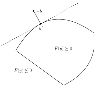
2.1. Example of a simple semidefinite problem for y ∈R2. Boundary of the
feasible set
y |F(y)0 is shown as a black curve. The minimal value of the objective functionb>y is attained aty∗. . . 12 2.2. Illustration of the logarithmic barrier function for different values of t. . 22 2.3. Hyperbolic paraboloid z=y22−y21. . . 23 2.4. Illustration of the sets DomF(y) and
y |X(y)0 . . . 24 2.5. Graph of the semidefinite optimization problem stated in Example 2.21. 27 2.6. Graph of execution times based on the size of semidefinite problems
solved by the selected toolboxes. . . 31 2.7. Graph of numbers of iterations required to solve the semidefinite
prob-lems by Algorithm 2.3 for different values of problem size k based on ε
using the implementation from the Polyopt package. . . 32 2.8. Example of a simple semidefinite problem with steps of Algorithm 2.3.
The algorithm starts from the analytic centeryF∗ and finishes at the opti-mal pointy∗. Selected fractions of the distanceky∗−y∗Fkare represented by concentric circles. . . 33 2.9. Graph of numbers of iterations required to get within the distanceλky∗−
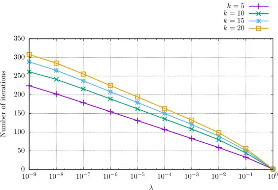
y∗Fkfrom the optimal solutiony∗ using Algorithm 2.3 for different values of problem sizekbased onλusing the implementation from the Polyopt package. . . 34 3.1. The intersection of the ellipse (3.21) and the hyperbola (3.22) with
solu-tions found by the eigenvalue and the eigenvector methods using multi-plication matrices. . . 38 3.2. Feasible region and the expected global minima of the problem (3.67). . 45 3.3. Graph of execution times of the polynomial optimization problems with
the relaxation order r = 1 based on the number of variables solved by the selected toolboxes. . . 51 3.4. Graph of execution times of the polynomial optimization problems in
n= 2 variables based on the degree of the polynomial in the objective function solved by the selected toolboxes. . . 53 4.1. Sculpture of Buddha head. Surface representing a point cloud
recon-structed from the taken images. . . 63 4.2. Scheme of the P3P problem. A pose of a calibrated camera can be
computed from three known 3D pointsX1,X2,X3 and their projections x1, x2, x3 into the image plane π. The camera projection center is
denoted asC. Distances d12, d23,d13 denote the distances between the
respective 3D points. . . 64 4.3. Histogram of the maximal reprojection errors of all correspondences in
the image for the best camera positions and rotations estimated by the selected polynomial solvers for the P3P problem compared to the maxi-mal reprojection errors computed for the ground truth camera positions and rotations. . . 67
ground truth camera positions. . . 68 4.5. Histogram of the errors in rotation angles computed by the selected
poly-nomial solvers for the P3P problem with respect to the ground truth camera rotations. . . 69 4.6. Histogram of the execution times required to compute the P3P problem
by the selected polynomial solvers. . . 70 4.7. Histogram of maximal degrees of relaxed monomials of the P3P
prob-lem. It corresponds to the value of variable t in the last iteration of Algorithm 3.4 for the Polyopt package and the MATLAB with MOSEK implementation. For the Gloptipoly toolbox it corresponds to two times the given relaxation order. . . 71 4.8. Scheme of the P3.5Pf problem. A pose of a calibrated camera with
unknown focal length can be computed from four known 3D pointsX1, X2, X3,X4 and their projections x1,x2,x3,x4 into the image planeπ.
The camera projection center is denoted asC. . . 72 4.9. Histogram of the maximal reprojection errors of all correspondences in
the image for the best camera positions and rotations estimated by the selected polynomial solvers for the P3.5Pf problem compared to the max-imal reprojection errors computed for the ground truth camera positions and rotations. . . 73 4.10. Histogram of the relative focal length errors computed by the selected
polynomial solvers for the P3.5Pf problem with respect to the ground truth focal lengths. . . 74 4.11. Histogram of the errors in estimated camera positions computed by the
selected polynomial solvers for the P3.5Pf problem with respect to the ground truth camera positions. . . 75 4.12. Histogram of the errors in rotation angles computed by the selected
poly-nomial solvers for the P3.5Pf problem with respect to the ground truth camera rotations. . . 75 4.13. Histogram of the execution times required to compute the P3.5Pf
prob-lem by the selected polynomial solvers. . . 76 4.14. Histogram of maximal degrees of relaxed monomials of the P3.5Pf
prob-lem. It corresponds to the value of variable t in the last iteration of Algorithm 3.4 for the Polyopt package and the MATLAB with MOSEK implementation. For the Gloptipoly toolbox it corresponds to two times the given relaxation order. . . 76
2.1. Execution times of different sizes of semidefinite problems solved by the
selected toolboxes. . . 30
3.1. Execution times of the polynomial optimization problems in different number of variables with the relaxation orderr= 1 solved by the selected toolboxes. . . 50
3.2. Execution times of the polynomial optimization problems for different degrees of the polynomial in the objective function in n = 2 variables solved by the selected toolboxes. . . 52
4.1. Table of numbers of all real and complex solutions and of numbers of found real solutions by each of the selected polynomial solver for the P3P problem. . . 68
4.2. Table of numbers of all real and complex solutions and of numbers of found real solutions by each of the selected polynomial solver for the P3.5Pf problem. . . 77
List of Algorithms
2.1. Newton method for minimization of self-concordant functions. . . 152.2. Damped Newton method for analytic centers. [36, Scheme 4.2.25] . . . . 18
2.3. Path following algorithm. [36, Scheme 4.2.23] . . . 20
3.4. The moment matrix algorithm for computing real roots. [30, Algorithm 1] 58
List of Listings
2.1. Installation of the package Polyopt. . . 252.2. Typical usage of the class SDPSolverof the Polyopt package. . . 25
2.3. Code for solving semidefinite problem stated in Example 2.21. . . 28
3.1. Typical usage of the class POPSolverof the Polyopt package. . . 48
3.2. Code for solving polynomial optimization problem stated in Example 3.16. 49 3.3. Typical usage of the class PSSolverof the Polyopt package. . . 61 3.4. Code for solving system of polynomial equations stated in Example 3.35. 61
BA Bundle adjustment.
C Set of complex numbers.
cl(S) Closure of the setS.
deg(p) Total degree of the polynomialp.
diag(x) Diagonal matrix with components of the vector x on the di-agonal.
domf Domain of the functionf. Domf cl(domf).
f0(x) First derivative of the function f(x).
f00(x) Second derivative of the functionf(x). G-J elimination Gauss-Jordan elimination.
I(V) Vanishing ideal of the varietyV.
In Identity matrix of sizen×n.
√
I Radical ideal of the idealI.
R
√
I Real radical ideal of the idealI.
hf1, f2, . . . , fni Ideal generated by the polynomials f1, f2, . . . , fn.
intS Interior of the setS.
ker(QΛ) Kernel of the quadratic formQΛ.
ker(M) Kernel of the matrix M.
λi(A) n
i=1 Set of all eigenvalues of the matrixA∈R
n×n.
LMI Linear matrix inequality.
LP Linear program.
N Set of natural numbers (including zero).
NB(f) Normal form of the polynomialf modulo idealI with respect to the basisB.
Pn Cone of positive semidefiniten×nmatrices.
PnP problem The perspective-n-point problem. P3P problem The perspective-three-point problem.
P3.5Pf problem The perspective-three-and-half-point problem with unknown focal length.
POP Polynomial optimization.
QCQP Quadratically constrained quadratic program.
R Set of real numbers.
R[x] Ring of polynomials with coefficients inR in nvariables x∈ Rn.
R[x]∗ Dual vector space to the ring of polynomialsR[x].
RANSAC Random Sample Consensus.
Sn Space ofn×nreal symmetric matrices.
SDP Semidefinite programming. SfM Structure from motion.
SGM method Semi-global matching method.
SO(3) Group of all rotations about the origin of three-dimensional space.
vec(p) Vector of the coefficients of the polynomial p with respect to some monomial basis.
VC(I) Algebraic variety of the idealI.
VR(I) Real algebraic variety of the idealI.
x(i) i-th element of the vector x.
x> Transpose of the vectorx.
dxe min{m∈Z|m≥x}; ceiling function.
bxc max{m∈Z|m≤x}; floor function.
Xf Multiplication matrix by the polynomialf.
In geometry of computer vision, many problems are formulated as systems of poly-nomial equations. The state of the art methods are based on polypoly-nomial algebra, i.e. on Gr¨obner bases and multiplication matrices computation. Contrary to this approach, this work applies non-linear optimization techniques to solve the polynomial systems, which is a novel idea in the field of geometry of computer vision. Moreover, the appli-cation of the optimization techniques allows us to enrich the polynomial systems with polynomial inequalities or to solve polynomial optimization problems, i.e. optimizing a polynomial function with given polynomial constraints.
1.1. Motivation
Object recognition and localization, reconstruction of 3D scenes, self-driving cars, film production, augmented reality and robotics are only few of many applications of geometry of computer vision. Thus, one would like to solve geometric problems effi-ciently, since these problems often have to be solved in real-time applications. Typical geometric problems from computer vision are the minimal problems, which arise when estimating geometric models of scenes from given images. To be able to solve these problems computationally, they are often represented by systems of algebraic equa-tions. Hence, one of the issues of computer vision is, how to solve systems of polynomial equations efficiently, which is the scope of this work.
The polynomial systems obtained from the geometric problems are often not trivial, but usually consist of many polynomial equations of high degree in several unknowns. From that reason, general algorithms for polynomial systems solving are not efficient for them, and therefore special solvers have been developed for different problems to solve these problems efficiently and robustly. Previously, these solvers were handcrafted, which is quite time demanding process that has to be done for each problem from scratch. Then, the process was automated by automatic generators [22, 23], which automatically generate efficient solver for a given type of the polynomial system. These solvers obtain the Gr¨obner basis of the system and then construct the multiplication matrix, from which solutions are extracted by eigenvectors computation. The side effect of this approach is that some non-real solutions often appear amongst real solutions, which are not solutions to the original geometric problem. Since the computation of the non-real solutions takes time, a method which would find real solutions only may be faster than the contemporary approach.
Some of the arisen systems may be overconstrained. Such systems have a solution when solved on precise data using precise arithmetic, but they have no solution when solved on real noisy data. However, these systems may be transformed into optimiza-tion problem by relaxing some of the constrains and by minimizing the error of these constraints. Therefore, an efficient polynomial optimization method may prove useful for overconstrained systems.
1.2. Contributions
To solve polynomial systems over real numbers only, we apply the moment method introduced by J. B. Lasserre et al. This method uses hierarchies of semidefinite pro-grams to find a Gr¨obner basis of real radical ideal constructed from the ideal generated by the given polynomials. Then, a multiplication matrix is constructed and solutions are obtained from it. In this case, the multiplication matrix should have smaller size than a multiplication matrix obtained from the automatic generator, which can save some computation time. We implement this method in Python and MATLAB and examine its properties on several minimal problems from geometry of computer vision on real 3D scenes. We show that this method is applicable on problems from computer vision.
The second contribution of this work is, that we describe and review a method for polynomial optimization problems. This method solves hierarchies of semidefinite pro-grams to find the optimal value. An application of this method can, for example, be a solver of overconstrained polynomial systems. We implement our own implementation of this method in Python and compare it to the state of the art methods on synthetic polynomial optimization problems.
Since semidefinite programs solving is a key element in both previously mentioned methods, we review and describe an interior-point method for semidefinite programs solving. To be able to use this method in implementations of the moment method and the polynomial optimization method, we implement this interior-point method in Python. To verify our implementation we compare it to the state of the art semidefinite solvers on synthetic semidefinite programs.
1.3. Thesis structure
In this work, we first review an interior-point method for semidefinite programs solv-ing. To do so, general properties of self-concordant functions and barriers need to be introduced, since they are key elements in convex optimization. Then, a specialized barrier function for semidefinite programming will be described. We describe our im-plementation of the semidefinite programs solver and compare it to the state of the art methods.
Secondly, we focus on polynomial optimization. After an introduction to polynomial algebra and moment matrices, we describe and implement a method, which solves polynomial optimization problems by relaxations of semidefinite programs. Then, we review the moment method and describe its implementation in Python.
To compare the implementation of the moment method to the state of the art meth-ods, we introduce two minimal problems from computer vision on which we perform the experiments. The minimal problems are the estimation (i) of the calibrated camera pose and (ii) of the calibrated camera pose with unknown focal length. We show that our implementation of the moment method is applicable to these selected geometric problems from computer vision.
The goal of the semidefinite programming (SDP) is to optimize a linear function on a given set, which is an intersection of a cone of positive semidefinite matrices with an affine space. This set is called a spectrahedron and it is a convex set. SDP, which is optimizing a convex function on a convex set, is a special case of convex optimization. Since SDP can be solved efficiently in polynomial time using interior-point meth-ods, it has many applications in practise. For example, any linear program (LP) and quadratically constrained quadratic program (QCQP) can be written as a semidefinite program. However, this may not be the best idea to do as more efficient algorithms exist for solving LPs and QCQPs. On the other hand, there exist many useful applications of SDP, e.g. many NP-complete problems in combinatorial optimization can be approx-imated by semidefinite programs. One of the combinatorial problem worth mentioning is the MAX CUT problem (one of the Karp’s original NP-complete problems [21]), for which M. Goemans and D. P. Williamson created the first approximation algorithm based on SDP [14]. Also in control theory, there are many problems based on linear matrix inequalities, which are solvable by SDP.
Special application of SDP comes from polynomial optimization since global solution of polynomial optimization problems can be found by hierarchies of semidefinite pro-grams. Systems of polynomial equations can also be solved by hierarchies of semidefinite problems. This approach has the advantage that there exists a method that allows us to compute real solutions only. Since in many applications, we are not interested in non-real solutions, this method may be the right tool for polynomial systems solving. We will focus in details on SDP application in polynomial optimization and polynomial systems solving in Chapter 3.
2.1. Preliminaries on semidefinite programs
In this section, we introduce some notation and preliminaries about symmetric ma-trices and semidefinite programs. We will introduce further notation and preliminaries later on in the text when needed.
At the beginning, let us denote the inner product for two vectorsx,y∈Rn by
hx, yi=
n
X
i=1
x(i)y(i) (2.1)
and the Frobenius inner product for two matrices X,Y ∈Rn×m by
hX, Yi= n X i=1 m X j=1 X(i,j)Y(i,j). (2.2) 2.1.1. Symmetric matrices
LetSn denotes the space of n×nreal symmetric matrices.
For a matrix M ∈ Sn, the notation M 0 means that M is positive semidefinite.
1. x>M x≥0 for allx∈Rn.
2. All eigenvalues ofM are nonnegative.
The set of all positive semidefinite matrices is a cone. We will denote it as Pnand it is
called the cone of positive semidefinite matrices.
For a matrixM ∈ Sn, the notationM 0 means thatM is positive definite. M 0
if and only if any of the following equivalent properties holds true: 1. M 0 and rankM =n.
2. x>M x >0 for allx∈Rn.
3. All eigenvalues ofM are positive.
2.1.2. Semidefinite programs
The standard (primal) form of a semidefinite program in variableX∈ Sn is defined
as follows: p∗= sup X∈Sn hC, Xi s.t. hAi, Xi=b(i) (i= 1, . . . , m) X0 (2.3)
where C,A1, . . . , Am ∈ Sn and b∈Rm are given.
The dual form of the primal form is the following program in variable y∈Rm.
d∗= inf y∈Rm b>y s.t. m X i=1 Aiy(i)−C0 (2.4) The constraint F(y) = m X i=1 Aiy(i)−C0 (2.5)
of the problem (2.4) is called a linear matrix inequality (LMI) in the variable y. The feasible region defined by LMI is called a spectrahedron. It can be shown, that this constraint is convex since if F(x)0 and F(y)0, then∀α,0≤α≤1 there holds
F αx+ (1−α)y
=αF(x) + (1−α)F(y)0. (2.6)
The objective function of the problem (2.4) is linear, and therefore convex too. Because the semidefinite program (2.4) has convex objective function and convex constraint, it is a convex optimization problem and can be solved by standard convex optimization methods. See Figure 2.1 to get a general picture, how a simple semidefinite problem may look like.
The optimal solution y∗ of any semidefinite program lies on the boundary of the feasible set, supposing the problem is feasible and the solution exists. The boundary of the feasible set is not smooth in general, but it is piecewise smooth as each piece is an algebraic surface.
Example 2.1 (Linear programming). Semidefinite programming can be seen as
−b
y∗
F(y)0
F(y)60
Figure 2.1. Example of a simple semidefinite problem fory∈R2. Boundary of the feasible set
y |F(y)0 is shown as a black curve. The minimal value of the objective functionb>y
is attained aty∗.
vectors in linear programming are replaced by LMI. Consider a linear program in the standard form y∗ = arg min y∈Rm b>y s.t. Ay−c≥0 (2.7) withb∈Rm,c∈ RnandA=a1 · · · am
∈Rn×m. This program can be transformed
into the semidefinite program (2.4) by assigning
C= diag(c), (2.8)
Ai = diag(ai). (2.9)
2.2. State of the art review
An early paper by R. Bellman and K. Fan about theoretical properties of semidefinite programs [5] was issued in 1963. Later on, many researchers worked on the problem of minimizing the maximal eigenvalue of a symmetric matrix, which can be done by solving a semidefinite program. Selecting a few from many: J. Cullum, W. Donath, P. Wolfe [10], M. Overton [39] and G. Pataki [40]. In 1984, the interior-point methods for LPs solving were introduced by N. Karmarkar [20]. It was the first reasonably effi-cient algorithm that solves LPs in polynomial time with excellent behavior in practise. The interior-point algorithms were then extended to be able to solve convex quadratic programs.
In 1988, Y. Nesterov and A. Nemirovski [37] did an important breakthrough. They showed that interior-point methods developed for LPs solving can be generalized to all convex optimization problems. All that is required, is the knowledge of a self-concordant barrier function for the feasible set of the problem. Y. Nesterov and A. Nemirovski have shown that a self-concordant barrier function exists for every convex set. However, their proposed universal self-concordant barrier function and its first and second derivatives are not easily computable. Fortunately for SDP, which is an important class of convex optimization programs, computable self-concordant barrier functions are known, and therefore the interior-point methods can be used.
Nowadays, there are many libraries and toolboxes that one can use for solving semidefinite programs. They differ in methods used and their implementations. Be-fore starting solving a problem, one should know the details of the problem to solve and choose the library accordingly to it as not every method and its implementation is suitable for every problem.
Most methods are based on interior-point methods, which are efficient and robust for general semidefinite programs. The main disadvantage of these methods is that they need to store and factorize usually large Hessian matrix. Most modern implementations of the interior-point methods do not need the knowledge of an interior feasible point in advance. SeDuMi [46] casts the standard semidefinite program into the homogeneous self-dual form, which has a trivial feasible point. SDPA [50] uses an infeasible interior-point method, which can initialized by an infeasible interior-point. Some of the libraries (e.g. MOSEK [34]) have started out as LPs solvers and were extended for QCQPs solving and convex optimization later on.
Another type of methods used in SDP are the first-order methods. They avoid storing and factorizing Hessian matrices, and therefore they are able to solve much larger problems than interior-point methods, but at some cost in accuracy. This method is implemented, for instance, in the SCS solver [38].
2.3. Interior point method
In this section, we will follow Chapter 4 of [36] by Y. Nesterov, which is devoted to the convex optimization problems. This chapter describes the state of the art interior-point methods for solving convex optimization problems. We will extract from it the only minimum, just to be able to introduce an algorithm for semidefinite programs solving. We will present some basic definitions and theorems but we will not prove them. Look into [36] for the proofs and more details.
2.3.1. Self-concordant functions
Definition 2.2 (Self-concordant function in R).A closed convex functionf:R7→
R is self-concordant if there exist a constantMf ≥0 such that the inequality
|f000(x)| ≤Mff00(x)3/2 (2.10)
holds for all x∈domf.
For better understanding of the self-concordant functions, we provide several exam-ples.
Example 2.3.
1. Linear and convex quadratic functions.
f000(x) = 0 for allx (2.11)
2. Negative logarithms. f(x) =−ln(x) forx >0 (2.12) f0(x) =−1 x (2.13) f00(x) = 1 x2 (2.14) f000(x) =−2 x3 (2.15) |f000(x)| f00(x)3/2 = 2 (2.16)
Negative logarithms are self-concordant functions with constant Mf = 2.
3. Exponential functions. f(x) =ex (2.17) f00(x) = f000(x) =ex (2.18) |f000(x)| f00(x)3/2 =e −x/2 →+∞ asx→ −∞ (2.19)
Exponential functions are not self-concordant functions.
Definition 2.4 (Self-concordant function inRn).A closed convex functionf: Rn7→
R is self-concordant if functiong:R7→R
g(t) =f(x+tv) (2.20) is self-concordant for allx∈domf and allv∈Rn.
Now, let us focus on the main properties of self-concordant functions.
Theorem 2.5 ([36, Theorem 4.1.1]).Let functionsfibe self-concordant with constants
Mi and letαi>0,i= 1,2. Then, the function
f(x) =α1f1(x) +α2f2(x) (2.21)
is self-concordant with constant
Mf = max 1 √ α1 M1; 1 √ α2 M2 (2.22) and
domf = domf1∩domf2. (2.23)
Corollary 2.6 ([36, Corollary 4.1.2]).Let function f be self-concordant with some
constant Mf and let α > 0. Then, the function φ(x) = αf(x) is also self-concordant
with the constant Mφ= √1αMf.
We call function f(x) as the standard self-concordant function if f(x) is some self-concordant function with the constantMf = 2. Using Corollary 2.6, we can see that any
self-concordant function can be transformed into the standard self-concordant function by scaling.
Theorem 2.7 ([36, Theorem 4.1.3]).Let functionf be self-concordant. If domf con-tains no straight line, then the Hessian f00(x) is nondegenerate at anyx from domf.
For some self-concordant function f(x), for which we assume that domf contains no straight line (which implies that all f00(x) are nondegenerate, see Theorem 2.7), we introduce two local norms as
kukx = q u>f00(x)u, (2.24) kuk∗x = q u>f00(x)−1u. (2.25)
Consider the following minimization problem
x∗ = arg min
x∈domff(x) (2.26)
with self-concordant function f(x). Algorithm 2.1 describes an iterative process of solving the optimization problem (2.26). The algorithm is divided into two stages by the value of kf0(xk)k∗xk. The splitting parameter β guarantees quadratic convergence
rate for the second part of the algorithm. The parameter β is chosen from interval (0,λ¯), where ¯ λ= 3− √ 5 2 , (2.27)
which is a solution of the equation
λ
(1−λ)2 = 1. (2.28)
Algorithm 2.1. Newton method for minimization of self-concordant functions.
Input:
f a self-concordant function to minimize
x0∈domf a starting point
β ∈(0,λ¯) a parameter of size of the region of quadratic convergence
εa precision
Output:
x∗ an approximation to the optimal solution to the minimization problem (2.26)
1: k←0 2: while kf0(xk)k∗xk ≥β do 3: xk+1 ←xk−1+kf0(1x k)k∗xkf 00(x k)−1f0(xk) 4: k←k+ 1 5: end while 6: while kf0(xk)k∗xk > ε do 7: xk+1 ←xk−f00(xk)−1f0(xk) 8: k←k+ 1 9: end while 10: return x∗ ←xk
The first while loop (lines 2 – 5) represents damped Newton method, where at each iteration we have
where
β−ln(1 +β)>0 for β >0, (2.30) and therefore the global convergence of the algorithm is ensured. It can be shown that the local convergence rate of the damped Newton method is also quadratic, but the presented switching strategy is preferred as it gives better complexity bounds.
The second while loop of the algorithm (lines 6 – 9) is the standard Newton method with quadratic convergence rate.
The algorithm terminates when the required precisionε is reached.
2.3.2. Self-concordant barriers
To be able to introduce self-concordant barriers, let us denote Domf as the closure of domf, i.e. Domf = cl(domf).
Definition 2.8 (Self-concordant barrier [36, Definition 4.2.2]).LetF(x) be a
stan-dard self-concordant function. We call it a ν-self-concordant barrier for set DomF, if
sup
u∈Rn
2u>F0(x)−u>F00(x)u≤ν (2.31) for all x∈domF. The value ν is called the parameter of the barrier.
The inequality (2.31) can be rewritten into the following equivalent matrix notation
F00(x) 1
νF
0(x)F0(x)>. (2.32)
In Definition 2.8, the hessian F00(x) is not required to be nondegenerate. However, in case that F00(x) is nondegenerate, the inequality (2.31) is equivalent to
F0>(x)F00(x)−1F0(x)≤ν. (2.33) Let us explore, which basic functions are self-concordant barriers.
Example 2.9.
1. Linear functions.
F(x) =α+a>x, domF =Rn (2.34)
F00(x) = 0 (2.35)
From (2.32) and for a6= 0 follows, that linear functions are not self-concordant barriers.
2. Convex quadratic functions. ForA=A>0: F(x) =α+a>x+1 2x >Ax, domF = Rn (2.36) F0(x) =a+Ax (2.37) F00(x) =A (2.38)
After substitution into (2.33) we obtain
(a+Ax)>A−1(a+Ax) =a>A−1a+ 2a>x+x>Ax, (2.39) which is unbounded from above on Rn. Therefore, quadratic functions are not
3. Logarithmic barrier for a ray. F(x) =−lnx, domF = x∈R |x >0 (2.40) F0(x) =−1 x (2.41) F00(x) = 1 x2 (2.42)
From (2.33), when F0(x) and F00(x) are both scalars, we get
F0(x)2
F00(x) =
x2
x2 = 1. (2.43)
Therefore, the logarithmic barrier for a ray is a self-concordant barrier with pa-rameterν = 1 on domainx∈R |x >0 .
Now, let us focus on the main properties of the self-concordant barriers.
Theorem 2.10 ([36, Theorem 4.2.1]).Let F(x) be a self-concordant barrier. Then,
the function c>x+F(x) is a self-concordant function on domF.
Theorem 2.11 ([36, Theorem 4.2.2]).LetFi be aνi-self-concordant barriers, i= 1,2.
Then, the function
F(x) =F1(x) +F2(x) (2.44)
is a self-concordant barrier for convex set
DomF = DomF1∩DomF2 (2.45)
with the parameter
ν=ν1+ν2. (2.46)
Theorem 2.12 ([36, Theorem 4.2.5]).LetF(x) be a ν-self-concordant barrier. Then,
for any x∈DomF and y∈DomF such that
(y−x)>F0(x)≥0, (2.47)
we have
ky−xkx≤ν+ 2√ν. (2.48)
There is one special point of a convex set, which is important for solving convex minimization problems. It is called the analytic center of convex set and we will focus on its properties.
Definition 2.13 ([36, Definition 4.2.3]).Let F(x) be a ν-self-concordant barrier for
the set DomF. The point
x∗F = arg min
x∈DomFF(x) (2.49)
Theorem 2.14 ([36, Theorem 4.2.6]).Assume that the analytic center of a ν -self-concordant barrier F(x) exists. Then, for anyx∈DomF we have
kx−x∗Fkx∗
F ≤ν+ 2
√
ν. (2.50)
This property clearly follows from Theorem 2.12 and the fact thatF0(x∗F) = 0. Thus, if DomF contains no straight line, then the existence of x∗F (which leads to nondegenerate F00(x∗F)) implies that the set DomF is bounded.
Now, we describe the algorithm and its properties for obtaining an approximation to the analytic center. To find the analytic center, we need to solve the minimization problem (2.49). For that, we will use the standard implementation of the damped Newton method with a termination condition
kF0(xk)k∗xk ≤β forβ ∈(0,1). (2.51)
The pseudocode of the whole minimization process is shown in Algorithm 2.2.
Algorithm 2.2. Damped Newton method for analytic centers. [36, Scheme 4.2.25]
Input:
F a ν-self-concordant barrier
x0∈DomF a starting point β ∈(0,1) a centering parameter
Output:
x∗F an approximation to the analytic center of the set DomF
1: k←0 2: while kF0(xk)k∗xk > β do 3: xk+1 ←xk−1+kF01(x k)k∗xkF 00(x k)−1F0(xk) 4: k←k+ 1 5: end while 6: return x∗F ←xk
Theorem 2.15 ([36, Theorem 4.2.10]).Algorithm 2.2 terminates no later than after
N steps, where N = 1 β−ln(1 +β) F(x0)−F(x ∗ F) . (2.52)
The knowledge of the analytic center allows us to solve the standard minimization problem
x∗ = arg min
x∈Qc
>
x (2.53)
with bounded closed convex set Q≡DomF, which has nonempty interior, and which is endowed with a ν-self-concordant barrierF(x). Denote
f(t, x) =tc>x+F(x) for t≥0 (2.54) as a parametric penalty function. Using Theorem 2.10 we can see that f(t, x) is self-concordant in x. Let us introduce new minimization problem using the parametric penalty function f(t, x)
x∗(t) = arg min
This trajectory is called the central path of the problem (2.53). We will reach the solution x∗(t) → x∗ as t → +∞. Moreover, since the set Q is bounded, the analytic center x∗F of this set exists and
x∗(0) =x∗F. (2.56)
From the first-order optimality condition, any point of the central path satisfies equation
tc+F0 x∗(t)= 0. (2.57) Since the analytic center lies on the central path and can be found by Algorithm 2.2, all we have to do, to find the solution x∗, is to follow the central path. This enables us an approximate centering condition
kf0(t, x)k∗x=ktc+F0(x)k∗x ≤β, (2.58) where the centering parameter β is small enough.
Assuming x ∈ domF, one iteration of the path-following algorithm consists of two steps: t+ =t+ γ kck∗ x , (2.59) x+ =x−F00(x)−1 t+c+F0(x) . (2.60)
Theorem 2.16 ([36, Theorem 4.2.8]).Letx satisfy the approximate centering
condi-tion (2.58)
ktc+F0(x)k∗x≤β (2.61) with β <¯λ= 3−
√
5
2 . Then forγ, such that
|γ| ≤ √ β 1 +√β −β, (2.62) we have again kt+c+F0(x+)k∗x+ ≤β. (2.63)
This theorem ensures the correctness of the presented iteration of the path-following algorithm. For the whole description of the path-following algorithm please see Algo-rithm 2.3.
Theorem 2.17 ([36, Theorem 4.2.9]).Algorithm 2.3 terminates no more than afterN
steps, where N ≤ O √νln νkck∗x∗ F ε ! . (2.64)
The parameters β and γ in Algorithm 2.2 and Algorithm 2.3 can be fixed. The reasonable values are:
β= 1 9, (2.65) γ = √ β 1 +√β −β = 5 36. (2.66)
Algorithm 2.2 and Algorithm 2.3 can be easily used to solve the standard minimiza-tion problem (2.53), supposing we have a feasible point x0 ∈Q.
Algorithm 2.3. Path following algorithm. [36, Scheme 4.2.23]
Input:
F a ν-self-concordant barrier
x0 ∈domF a starting point satisfyingkF0(x0)k∗x0 ≤β, e.g. the analytic center x
∗
F
of the set DomF
β ∈(0,1) a centering parameter γ a parameter satisfying |γ| ≤ √ β 1+√β −β ε >0 an accuracy Output:
x∗ an approximation to the optimal solution to the minimization problem (2.53)
1: t0 ←0 2: k←0 3: while εtk < ν+(β+ √ ν)β 1−β do 4: tk+1←tk+kckγ∗ xk 5: xk+1 ←xk−F00(xk)−1 tk+1c+F0(xk) 6: k←k+ 1 7: end while 8: return x∗ ←xk
2.3.3. Barrier function for semidefinite programming
In this section, we are going to show how to find a self-concordant barrier for the semidefinite program (2.4) so that we can use Algorithm 2.2 and Algorithm 2.3 to solve it. For the purpose of this section, we are interested only in the constrains of the problem. The constrains are defining us the feasibility set
Q= y∈Rm |A0+ m X i=1 Aiy(i)0 , (2.67)
whereA0, . . . , Am ∈ Sn. Let us denoteX(y) =A0+Pmi=1Aiy(i). If the matrixX(y) is
block diagonal X(y) = X1(y) 0 · · · 0 0 X2(y) · · · 0 .. . ... . .. ... 0 0 · · · Xk(y) (2.68)
with Xj(y) ∈ Snj forj = 1, . . . , k and Pkj=1nj =n, then the feasibility set Q can be
expressed as
Q=
y∈Rm |X
j(y)0, j = 1, . . . , k . (2.69)
This rule allows us to easily add or remove some constraints without touching the others and to keep the sizes of the used matrices small, which can significantly speed up the computation.
Instead of the set Q, which is parametrized byy, we can directly optimize over the set of positive semidefinite matrices. This set Pn is defined as
and it is called the cone of positive semidefinite n×n matrices. This cone is a closed convex set with interior formed by positive definite matrices and on its boundary lie matrices that have at least one eigenvalue equal to zero.
Now, we are looking for a self-concordant barrier function, which will enable us to optimize over the conePn. The domain of this function needs to contain the setPnand
the values of the function have to be growing to +∞ as getting closer to the boundary of the set Pn. This will create us a repelling force from the boundary of Pn, when
following the central path (2.55). Consider the function
F(X) =−ln
n
Y
i=1
λi(X) (2.71)
as the self-concordant barrier function for the setPn, whereX ∈intPnand
λi(X) n i=1
is the set of eigenvalues of the matrix X. To avoid the computation of eigenvalues, the function F(X) can be also expressed as
F(X) =−ln det(X). (2.72)
Theorem 2.18 ([36, Theorem 4.3.3]).Function F(X) is an n-self-concordant barrier
for Pn.
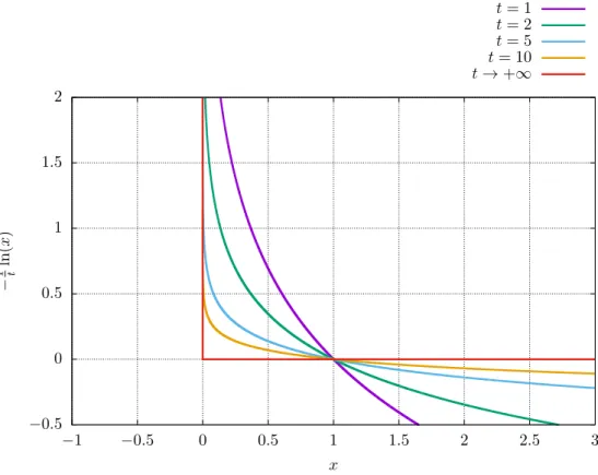
Example 2.19. Consider one-dimensional problem with linear constraintx≥0. Then,
the set Q is
Q={x∈R |x≥0} (2.73)
and one of the barrier functions for this set Qis
F(x) =−ln(x). (2.74)
Then, when following the central path (2.55), the function F(x) allows us to reach the boundary of Q as t grows to +∞. This situation is shown in Figure 2.2 for different values of t.
Note, that DomF ⊇ Pnbecause det(X)≥0 when the number of negative eigenvalues
ofXis even. Therefore, the set DomF is made by disjoint subsets, which one of them is
Pn. As Algorithm 2.2 and Algorithm 2.3 are interior point algorithms, when the starting
point is from intPn, then we never leavePnduring the execution of the algorithms and
the optimal solution is found.
Similarly, the self-concordant barrier function for the setQ is a function
F(y) =−ln det X(y)
. (2.75)
Example 2.20. To make it clearer, what is the difference between the set Q and
DomF(y), let us present an example. Let
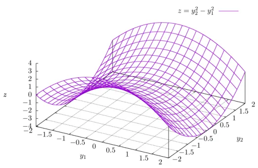
X(y) = y2 y1 y1 y2 , (2.76) where y= y1 y2 > . The equation z= det X(y)=y22−y12 (2.77)
−0.5 0 0.5 1 1.5 2 −1 −0.5 0 0.5 1 1.5 2 2.5 3 − 1 ln(t x ) x t= 1 t= 2 t= 5 t= 10 t→+∞
Figure 2.2. Illustration of the logarithmic barrier function for different values oft.
represents a hyperbolic paraboloid, which you can see in Figure 2.3. Therefore, the equation z= 0 is a slice of it, denoted by the purple color in Figure 2.4. The domain of the self-concordant barrier function is
DomF(y) = n
y | det X(y)≥0 o
(2.78) and is shaded blue. We can see, that the set DomF(y) consists of two disjoint parts. One of them is the set where X(y) 0 (denoted by the orange color) and the second part is an area where both eigenvalues ofX(y) are negative. Therefore, one has to pick his starting point x0 from the interior of the set Q =
y ∈ R2 |X(y) 0 to obtain
the optimal solution from the set Q.
When the matrix X has the block diagonal form (2.68), we can rewrite the barrier function (2.75) as F(y) =− k X j=1 ln det Xj(y) . (2.79)
For the purposes of Algorithm 2.2 and Algorithm 2.3, we need the first and the second partial derivatives of this function. Let us denote Xj(y) = Aj,0 +Pmi=1Aj,iy(i) for
j = 1, . . . , k, then the derivatives are:
∂F ∂y(u) y =− k X j=1 tr Xj(y)−1Aj,u , (2.80) ∂2F ∂y(u)∂y(v) y = k X j=1 trXj(y)−1Aj,u Xj(y)−1Aj,v , (2.81)
−2 −1.5 −1 −0.5 0 0.5 1 1.5 2 −2−1.5 −1 −0.5 0 0.5 1 1.5 2 −4 −3 −2 −1 0 1 2 3 4 z z=y22−y21 y1 y2 z
Figure 2.3. Hyperbolic paraboloidz=y22−y12.
for u, v= 1, . . . , m.
The computation of the derivatives is the most expensive part of each step of Algo-rithm 2.2 and AlgoAlgo-rithm 2.3. Therefore, the estimated number of aAlgo-rithmetic operations of computation of the derivatives is also the complexity of each step in the algorithms. The number of arithmetic operations for j-th constraint in formy |Xj(y)0 is as
follows:
• the computation ofXj(y) =Aj,0+Pmi=1Aj,iy(i) needs mn2 operations,
• the computation of the inversionXj(y)−1 needs n3 operations,
• to compute all matrices Xj(y)−1Aj,u foru= 1, . . . , mis neededmn3 operations,
• to compute tr Xj(y)−1Aj,u
foru= 1, . . . , m is neededmnoperations,
• the computation of tr Xj(y)−1Aj,u Xj(y)−1Aj,v for u, v = 1, . . . , m needs m2n2 operations.
The most expensive parts requires mn3 and m2n2 arithmetic operations on each con-straint. Typically, the value k, the number of constraints, is small and is kept constant when the semidefinite programs are generated as subproblems, when solving more com-plex problems, e.g. polynomial optimization. Therefore, we can say, that kis constant and we can omit it from the complexity estimation. To sum up, one step of Algo-rithm 2.2 and AlgoAlgo-rithm 2.3 requires
O m(m+n)n2 (2.82)
−2 −1.5 −1 −0.5 0 0.5 1 1.5 2 −2 −1.5 −1 −0.5 0 0.5 1 1.5 2 y2 y1 DomF(y) y |X(y)0 det X(y) = 0
Figure 2.4. Illustration of the sets DomF(y) andy |X(y)0 .
2.4. Implementation details
To be able to study the algorithms described previously in this section, we have implemented them in the programming language Python [47]. The full knowledge of the code allows us to trace the algorithms step by step and inspect their behaviors. Instead of using some state of the art toolboxes for semidefinite programming, e.g. SeDuMi [46] and MOSEK [34], which are more or less black boxes for us, the knowledge of the used algorithms allows us to decide, if the chosen algorithm is suitable for the given semidefinite problem or not. Moreover, if we would like to create some specialized solver for some class of semidefinite problems, we can easily reuse the code, edit it as required and build the solver very quickly. On the other hand, we can not expect that our implementation will be as fast as the implementation of some state of the art toolboxes, as much more time and effort was used to develop them.
The implementation is compatible with Python version 3.5 and higher. The package NumPy is used for linear algebra computations. Please refer to the installation guide of NumPy for your system to ensure, that it is correctly set to use the linear algebra libraries, e.g. LAPACK [3], ATLAS [48] and BLAS [31]. The incorrect setting of these libraries causes significant drop of the performance. Other Python packages are required as well, e.g. SymPy and SciPy, but theirs settings are not so crucial for the performance of this implementation.
2.4.1. Package installation
The package with implementation of Algorithm 2.2 and Algorithm 2.3 is named Polyopt, as the semidefinite programming part of this package is only a tool, which is used for polynomial optimization and polynomial systems solving, which will be described in Chapter 3. The newest version of the package is available athttp://cmp. felk.cvut.cz/~trutmpav/master-thesis/polyopt/. To install the package on your
system, you have to clone and checkout the Git repository with the source codes of the package. To install other packages that are required, the preferred way is to use the pip1 installer. The required packages are listed in the requirements.txt file. Then, install the package using the script setup.py. For the exact commands for the whole installation process please see Listing 2.1.
Listing 2.1. Installation of the package Polyopt.
1: git clone https://github.com/PavelTrutman/polyopt.git
2: cd polyopt
3: python3 setup.py install
To check, whether the installation was successful, run command python3 setup.py test, which will execute the predefined tests. If no error emerges, then the package is installed and ready to use.
2.4.2. Usage
The Polyopt package is able to solve semidefinite programs in the form
y∗ = arg min y∈Rmc >y s.t. Aj,0+ m X i=1 Aj,iy(i)0 forj= 1, . . . , k, (2.83)
where Aj,i ∈ Snj for i = 0, . . . m and j = 1, . . . , k, c ∈ Rm and k is the number of
constraints. In addition, a strictly feasible point y0 ∈Rm must be given.
The semidefinite program solver is implemented in the classSDPSolverof the Polyopt package. Firstly, the problem is initialized by the matrices Aj,i and the vectorc. Then,
the functionsolveis called with parametery0as the starting point and with the method
for the analytic center estimation. A choice from two methods is available, firstly, the method dampedNewton, which corresponds to Algorithm 2.2, and secondly, the method auxFollow, which is the implementation of the Auxiliary path-following scheme [36]. However, the auxFollowmethod is unstable and it fails in some cases, and therefore it is not recommended to use. The function solve returns the optimal solution y∗. The minimal working example is shown in Listing 2.2.
Listing 2.2. Typical usage of the classSDPSolverof the Polyopt package.
1: import polyopt
2:
3: # assuming the matrices Aij and the vectors c and y0 are already
defined
4: problem = polyopt.SDPSolver(c, [[A10, A11, ..., A1m], ..., [Ak0, Ak1, ..., Akm]])
5: yStar = problem.solve(y0, problem.dampedNewton)
Detailed information can be printed out during the execution of the algorithm. This option can be set by problem.setPrintOutput(True). Then, in each iteration of Algorithm 2.2 and Algorithm 2.3, the valuesk,xkand eigenvalues ofXj(xk) are printed
to the terminal.
1
If n, the dimension of the problem, is equal to 2, boundary of the set DomF
(2.78) and all intermediate points xk can be plotted. This is enabled by setting
problem.setDrawPlot(True). An example of such a graph is shown in Figure 2.5. The parameters β and γ are predefined to the same values as in (2.65) and (2.66). These parameters can be set to different values by assigning to the variablesproblem.beta and problem.gamma respectively. The default value for the accuracy parameter ε is 10−3. This value can be changed by overwriting the variableproblem.eps.
The functionproblem.getNu()returns theνparameter of the self-concordant barrier function used for the problem according to Theorem 2.18. When the problem is solved, we can obtain the eigenvalues ofX(y∗) by callingproblem.eigenvalues(). We should observe, that some of them are positive and some of them are zero (up to the numerical precision). The zero eigenvalues mean, that we have reached the boundary of the set
Q, because the optimal solution lies always on the boundary of the set Q.
It may happen, that the set DomF is not bounded, but the optimal solution can be attained. In this case, the analytic center does not exists and the proposed algorithms can not be used. By adding a constraint
Xk+1(y) = R2 y(1) y(2) · · · y(m) y(1) 1 0 · · · 0 y(2) 0 1 · · · 0 .. . ... ... . .. ... y(m) 0 0 · · · 1 forR∈R, (2.84)
we bound the set by a ball with radius R. The constraint (2.84) is equivalent to
kyk2
2 ≤R2. (2.85)
This will make the set DomF bounded and the analytic center can by found in the standard way by Algorithm 2.2. When optimizing the linear function by Algorithm 2.3, the radius R may be set too small and the optimum may be found on the boundary of the constraint (2.84). Then, the found optimum is not the solution to the original problem and the algorithm has to be run again with bigger value of R. The optimum is found on the boundary of the constraint (2.84), if at least one of the eigenvalues of
Xk+1(y∗) is zero. In our implementation, the artificial bounding constraint (2.84) can
be set by problem.bound(R). When the problem is solved, we can list the eigenvalues of Xk+1(y∗) by the functionproblem.eigenvalues(’bounded’).
Example 2.21.Let us present a simple example to show a detailed usage of the package
Polyopt. Let us have semidefinite program in a form
y∗= arg min y∈R2 y(1)+y(2) s.t. 1 +y(1) y(2) 0 y(2) 1−y(1) y(2) 0 y(2) 1−y(1) 0 (2.86)
with starting point
y0=
0 0>. (2.87)
Listing 2.3 shows the Python code used to solve the given problem. The graph of the problem is shown in Figure 2.5. The analytic center of the feasible region of the problem is
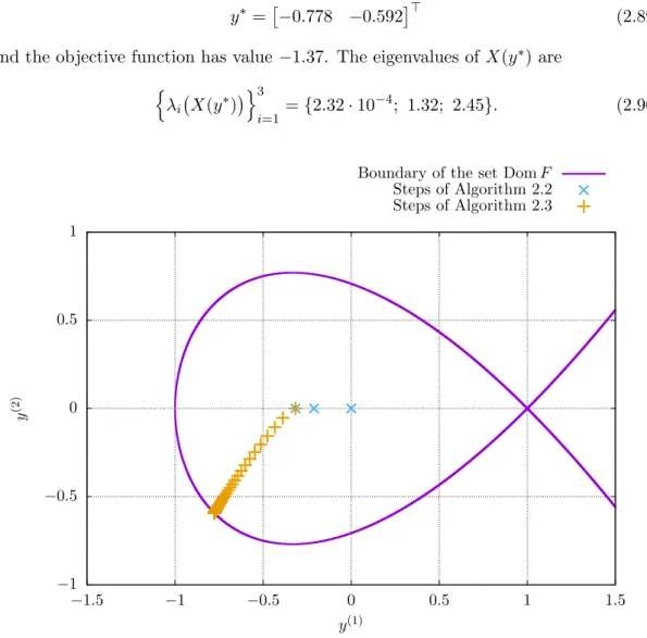
the optimal solution is attained at
y∗=
−0.778 −0.592> (2.89) and the objective function has value −1.37. The eigenvalues ofX(y∗) are
n λi X(y∗) o3 i=1 = {2.32·10−4; 1.32; 2.45}. (2.90) −1 −0.5 0 0.5 1 −1.5 −1 −0.5 0 0.5 1 1.5 y (2) y(1)
Boundary of the set DomF
Steps of Algorithm 2.2 Steps of Algorithm 2.3
Figure 2.5. Graph of the semidefinite optimization problem stated in Example 2.21.
2.5. Comparison with the state of the art methods
Because a new implementation of a well-known algorithm was made, one should compare many properties of this implementation with the contemporary state of the art implementations. For that reason, we have generated some random instances of semidefinite problems. We have solved these problems by our implementation from the Polyopt package and by selected state of the art toolboxes, namely SeDuMi [46] and MOSEK [34]. Firstly, we have verified the correctness of the implementation by checking that the optimal solution is the same as the solution obtained by SeDuMi and MOSEK for each instance of data. We have also measured execution times of all three libraries and compared them in Table 2.1 and Figure 2.6.
2.5.1. Problem description
Now, let us describe, how the random instances of the semidefinite problems were generated. From (2.82) we know that each step of Algorithm 2.2 and Algorithm 2.3
Listing 2.3. Code for solving semidefinite problem stated in Example 2.21.
1: from numpy import *
2: import polyopt
3:
4: # Problem statement
5: # min c1*y1 + c2*y2
6: # s.t. A0 + A1*y1 + A2*y2 >= 0 7: c = array([[1], [1]]) 8: A0 = array([[1, 0, 0], 9: [0, 1, 0], 10: [0, 0, 1]]) 11: A1 = array([[1, 0, 0], 12: [0, -1, 0], 13: [0, 0, -1]]) 14: A2 = array([[0, 1, 0], 15: [1, 0, 1], 16: [0, 1, 0]]) 17: 18: # starting point 19: y0 = array([[0], [0]]) 20:
21: # create the solver object
22: problem = polyopt.SDPSolver(c, [[A0, A1, A2]])
23:
24: # enable graphs
25: problem.setDrawPlot(True)
26:
27: # enable informative output
28: problem.setPrintOutput(True)
29:
30: # solve!
31: yStar = problem.solve(y0, problem.dampedNewton)
32:
33: # print eigenvalues of X(yStar)
requires m(m+n)n2 arithmetic operations, wherem is the size of the matrices in the LMI constraint and nis the number of variables. Since in typical applications of SDP, the size of the matrices grows with the number of variables, we have set m=nto have just single parameter, which we call the size of the problem.
In our experiment, we have generated 50 unique LMI constraints for each size of the problem from 1 to 25. Each unique constraint has form
Xk,l(y) =Ik+ k
X
i=1
Ak,l,iy(i) (2.91)
for the size of the problem k = 1, . . . ,25 and unique LMI constraint l = 1, . . . ,50, where Ak,l,i ∈ Sk. The matrices Ak,l,i were filled with random numbers from uniform
distribution (−1; 1) with symmetricity of the matrices preserved. The package Polyopt requires the starting pointy0 to be given by the user in advance. But from the structure
of the constraint (2.91) we can see that y0∈Rk
y0 =
0 · · · 0> (2.92) is a feasible point. We used the point y0 to initialize problems for Polyopt package
but we have let SeDuMi and MOSEK use their own initialization process. However, since the LMI constraints were randomly generated, there is no guarantee that the sets, which they define, are bounded. Therefore, we have added constraint (2.84) for
R = 103, which guarantees that we are optimizing over bounded sets.
The objective function of the problem is generated randomly too. For each unique instance, we have generated random vector r ∈ Rn from uniform distribution (−1; 1).
Then, the objective function to minimize isr>y. The final generated problem denoted as Pk,l looks like min y∈Rk r>k,ly s.t. Ik+ k X i=1 Ak,l,iy(i)0 R2 y(1) y(2) · · · y(k) y(1) 1 0 · · · 0 y(2) 0 1 · · · 0 .. . ... ... . .. ... y(k) 0 0 · · · 1 0. (2.93) 2.5.2. Time measuring
To eliminate influences that negatively affect the execution times on CPU, such as other processes competing for the same CPU core, processor caching, data loading delays, etc., we have executed each problemPk,l 50 times. So, for each problemPk,l we
have obtained execution timesτk,l,sfors= 1, . . . ,50. Because the influences mentioned
above can only prolong the execution times, we have selected minimum of τk,l,sfor each
problem Pk,l.
τk,l=
50
min
Since the execution times of problems of the same sizes should be more or less the same, we have computed the average execution time τk for each size of the problem.
τk= 1 50 50 X l=1 τk,l (2.95)
These execution times τk, where k is the size of the problem, were measured and
computed separately for the Polyopt, SeDuMi and MOSEK toolboxes and are shown in Table 2.1 and Figure 2.6.
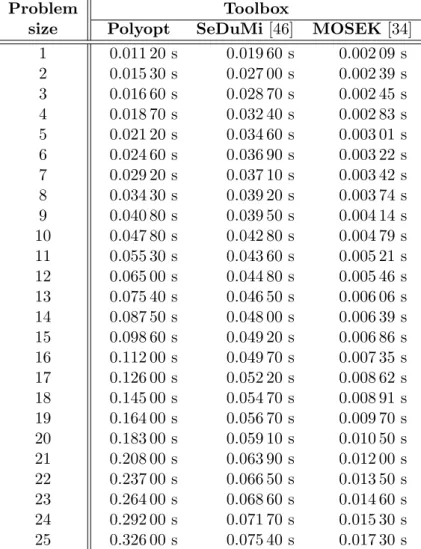
Problem Toolbox
size Polyopt SeDuMi[46] MOSEK[34]
1 0.011 20 s 0.019 60 s 0.002 09 s 2 0.015 30 s 0.027 00 s 0.002 39 s 3 0.016 60 s 0.028 70 s 0.002 45 s 4 0.018 70 s 0.032 40 s 0.002 83 s 5 0.021 20 s 0.034 60 s 0.003 01 s 6 0.024 60 s 0.036 90 s 0.003 22 s 7 0.029 20 s 0.037 10 s 0.003 42 s 8 0.034 30 s 0.039 20 s 0.003 74 s 9 0.040 80 s 0.039 50 s 0.004 14 s 10 0.047 80 s 0.042 80 s 0.004 79 s 11 0.055 30 s 0.043 60 s 0.005 21 s 12 0.065 00 s 0.044 80 s 0.005 46 s 13 0.075 40 s 0.046 50 s 0.006 06 s 14 0.087 50 s 0.048 00 s 0.006 39 s 15 0.098 60 s 0.049 20 s 0.006 86 s 16 0.112 00 s 0.049 70 s 0.007 35 s 17 0.126 00 s 0.052 20 s 0.008 62 s 18 0.145 00 s 0.054 70 s 0.008 91 s 19 0.164 00 s 0.056 70 s 0.009 70 s 20 0.183 00 s 0.059 10 s 0.010 50 s 21 0.208 00 s 0.063 90 s 0.012 00 s 22 0.237 00 s 0.066 50 s 0.013 50 s 23 0.264 00 s 0.068 60 s 0.014 60 s 24 0.292 00 s 0.071 70 s 0.015 30 s 25 0.326 00 s 0.075 40 s 0.017 30 s
Table 2.1. Execution times of different sizes of semidefinite problems solved by the selected toolboxes.
It has to be mentioned, that the Polyopt toolbox is implemented in Python, but the toolboxes SeDuMi and MOSEK were run from MATLAB with precompiled MEX files (compiled C, C++ or Fortran code) and therefore the execution times are not readily
comparable. On the other side, the Python package NumPy uses common linear algebra libraries, like LAPACK [3], ATLAS [48] and BLAS [31], and we can presume that SeDuMi and MOSEK use them too.
Our intention was to measure only the execution time of the solving phase, not of the setup time. In case of the Polyopt package, we measured the execution time of the function solve(). For SeDuMi and MOSEK, we have used MATLAB framework
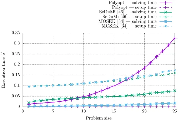
0 0.05 0.1 0.15 0.2 0.25 0.3 0.35 0 5 10 15 20 25 Execution time [s] Problem size
Polyopt — solving time Polyopt — setup time SeDuMi [46] — solving time SeDuMi [46] — setup time MOSEK [34] — solving time MOSEK [34] — setup time
Figure 2.6. Graph of execution times based on the size of semidefinite problems solved by the selected toolboxes.
YALMIP [32] for defining the semidefinite programs and calling the solvers. The exe-cution time of the YALMIP code is quite long, because YALMIP makes an analysis of the problem and compiles it into a standard form. Only after that, an external solver (SeDuMi or MOSEK) is called to solve the problem. Fortunately, YALMIP internally measures the execution time of the solver, so we have used this time in our statistics. For overall comparison we have also measured the setup time, e.g. the execution time spent before the SDP solver is actually called, of all three packages and we have shown them in Figure 2.6.
The experiments were executed on Intel Xeon E5-1650 v4 CPU 3.60GHz based com-puter with sufficient amount of free system memory. The installed version of Python was 3.5.3 and MATLAB R2017b 64-bit was used.
2.5.3. Results
By the look of the solving times shown in Figure 2.6, we can see that the MOSEK toolbox totally wins. The SeDuMi toolbox seems to have some constant overhead, but the execution time grows slowly with the increasing size of the problem. The Polyopt package accomplishes quite bad results compared to SeDuMi and MOSEK, especially for large sizes of problems. But this behavior was expected, as we know that the execution time should be proportional to k4, wherekis the size of the problem. However, due to SeDuMi overhead, the Polyopt package is faster than SeDuMi for problem sizes up to eight.
Regarding the setup times of the solvers, we can observe that the YALMIP framework spends more execution time by analyzing and compiling the problem than by solving it. This makes inadequate overhead for small problems, but it may prove crucial for solving large problems with many unknowns.
2.6. Speed–accuracy trade-off
Obtaining a precise solution of a semidefinite program is quite time consuming, es-pecially for problems with many unknowns, as we can see from Figure 2.6. However, in many applications we have no need for a precise solution. We only need a “good enough” solution, but obtained in a limited time period. Therefore one should be interested in a analysis describing this speed–accuracy trade-off.
2.6.1. Precision based analysis
The first experiment is an observation how many iterations, and therefore how much time, is required to find a solution based on the value of ε from Algorithm 2.3. This value of ε represents an accuracy of Algorithm 2.3 and sets up a threshold for the termination condition. The bigger the value ofεthe less iterations the algorithm needs to terminate, and therefore less computation time is spent.
To evaluate the dependency we have generated unique semidefinite programs Pk,l
according to (2.93) for k = 5,10,15,20 and l = 1, . . . ,1000. For each of this problem and accuracy ε we have measured the number of iterations Nk,l,ε of Algorithm 2.3
required to find the solution. Then, we have averaged the numbers across the unique problems. Nk,ε = 1 1000 1000 X l=1 Nk,l,ε (2.96)
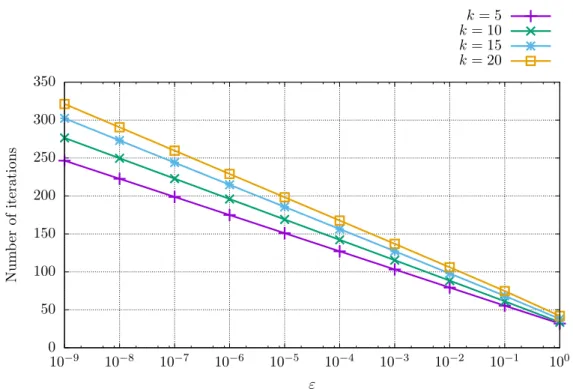
The values ofNk,ε are plotted in Figure 2.7 for different values of kand ε.
0 50 100 150 200 250 300 350 10−9 10−8 10−7 10−6 10−5 10−4 10−3 10−2 10−1 100 Num b er of iteration s ε k= 5 k= 10 k= 15 k= 20
Figure 2.7. Graph of numbers of iterations required to solve the semidefinite problems by Algorithm 2.3 for different values of problem size k based on ε using the implementation from the Polyopt package.
From the plot we can see that the number of iterations, and therefore the execution time, required to solve a given problem of fixed problem sizekis proportional to log(ε).
This results is in accordance with the estimated number of steps from the equation (2.64).
2.6.2. Analysis based on the required distance from the solution
Algorithm 2.3 starts at the analytic centeryF∗ of the feasible set of the problem and then follows the central path until it is sufficiently close to the optimal solution y∗. The sizes of the steps of the algorithm are decreasing as the algorithm is closing to the solution. Therefore, we need only few iterations to get within half the distanceky∗−y∗Fk
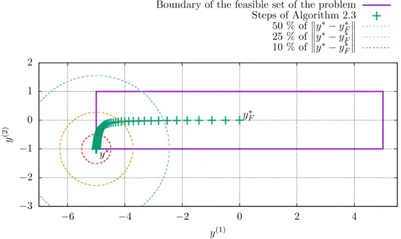
from the solution, but many of them to be within 1 % of the distance ky∗−y∗Fk from the solution. The situation for a simple semidefinite problem is shown in Figure 2.8.
−3 −2 −1 0 1 2 −6 −4 −2 0 2 4 y (2) y(1)
Boundary of the feasible set of the problem Steps of Algorithm 2.3 50 % ofky∗−y∗Fk 25 % ofky∗−y∗Fk 10 % ofky∗−y∗Fk y∗F y∗
Figure 2.8. Example of a simple semidefinite problem with steps of Algorithm 2.3. The algorithm starts from the analytic center y∗F and finishes at the optimal point y∗. Selected fractions of the distanceky∗−y∗Fkare represented by concentric circles.
To see how many iterations are needed to get within some fraction of the distance
ky∗−y∗Fkfrom the optimal solutiony∗, we have generated unique semidefinite problems
Pk,lfor the problem sizesk= 5,10,15,20 andl= 1, . . . ,1000 according to (2.93). Then,
we have solved each problem with accuracyε= 10−9to obtain a precise approximation
of the solutiony∗. After that we have counted how many iterationsNk,l,λ are needed to
get within the distance λky∗−y∗Fk from the solution y∗ for the given problem and for selected values ofλ. Then, we have averaged the numbers across the unique problems.
Nk,λ= 1 1000 1000 X l=1 Nk,l,λ (2.97)
The values ofNk,λ are plotted in Figure 2.9 for different values ofk and λ.
From the experiments we can see that the number of iterations, and therefore the execution time, of Algorithm 2.3 required to get within some fractionλof the distance