Spurious and hidden volatility
M. Angeles Carnero
1, Daniel Pe˜na
2and Esther Ruiz
2∗1Dpt. Fundamentos del An´alisis Econ´omico,
Universidad de Alicante
2Dpt. Estad´ıstica
Universidad Carlos III de Madrid
[email protected] [email protected]
May 25, 2004
Abstract
This paper analyzes the effects caused by the presence of outliers on the iden-tification and estimation of GARCH models. We show that outliers can lead to detect spurious conditional heteroscedasticity and they can also hide gen-uine ARCH effects. First, we derive the asymptotic biases caused by outliers on the sample autocorrelations of squared observations and their effects on some popular homoscedasticity tests. Then, we obtain the asymptotic biases of the OLS estimates of the parameters of ARCH(p) models and analyze their
∗Part of this work was done while the first author was visiting Nuffield College during the summer 2003. She is indebted to Neil Shephard for financial support and very useful discussions. We are very grateful to Andr´es Alonso, Michael McAleer, Ana P´erez and the seminar participants at Universidad de Alicante, Universidad Aut´onoma de Madrid and Erasmus University Rotterdam for helpful comments and suggestions. Financial support from proyect BEC2002.03720 by the Spanish Government is gratefuly acknowledged by the third author. Any remaining errors are our own.
finite sample behavior by means of extensive Monte Carlo experiments. The finite sample results are also extended to GLS and ML estimates of ARCH(p) and GARCH(1,1) models. All the results are illustrated analyzing real series of financial returns.
1
Introduction
Generalized AutoRegressive Conditional Heteroskedasticity (GARCH) mod-els were introduced by Engle (1982) and Bollerslev (1986) to represent the dynamic evolution of conditional variances and they have been extensively used in the empirical analysis of high frequency financial returns. However, we often find that when these models are fitted to real time series, the residu-als still have excess kurtosis, which could be explained, among other reasons, by the presence of outliers; see, for example, Bollerslev (1987), Ter¨asvirta (1996) and Franses and Ghijsels (1999).
Previous results on the effects of outliers on the identification and estima-tion of condiestima-tional heteroscedasticy are somehow confusing. Some authors argue that outliers generate spurious heteroscedasticity. For example, Balke and Fomby (1994) conclude that the outliers in several macroeconomic series of the US economy are able to explain most of the observed non-linearities. A similar conclusion is reached by Franses and Gijsels (1999) for macroeco-nomic series and Aggarwal et al. (1999) and Franses and Van Dijk (2000) for financial returns. On the other hand, other authors suggest that the presence of outliers may hide genuine heterocedasticity; see, for example, Mendes (2000) and Li and Kao (2002) for an empirical application with ex-change rates returns.
The simultaneous presence of conditional heteroscedasticity and outliers in time series can be easily confused because both phenomena cause excess kurtosis and, if outliers appear in patches, autocorrelated squared observa-tions. The objective of this paper is to show that the presence of additive
outliers in uncorrelated GARCH series may generate spurious heteroscedas-ticity when they appear in patches, and hide legitimate heterocedasheteroscedas-ticity when they are isolated. Consequently, both the size and power of tests for conditional homoscedasticity can be distorted in the presence of outliers. Also, they modify the estimated autocorrelations of squares and the esti-mated parameters of the conditional variance.
The paper is organized as follows. Section 2 defines different types of outliers in the context of the popular ARCH(p) and GARCH(1,1) models. In this paper, we focus on level outliers that do not affect the conditional variance. Section 3 analyses the effects of level outliers on the sample au-tocorrelations of squared observations and on several tests for conditional heteroscedasticity. In section 4, we derive the asymptotic bias of the Ordi-nary Least Squares (OLS) estimator of the parameters of ARCH(p) models contaminated by level outliers. Its finite sample properties are also ana-lyzed by means of extensive Monte Carlo experiments. These results are also extended to the Maximum Likelihood (ML) estimator. Section 5 anal-yses the finite sample properties of the ML estimator of the parameters of GARCH(1,1) models. Section 6 illustrates the results by analyzing several real series of financial returns. Finally, Section 7 concludes the paper.
2
GARCH models and outliers
The most popular model to represent the dynamic evolution of conditional variances is the GARCH(1,1) model proposed independently by Bollerslev (1986) and Taylor (1986). This model specifies the series of interest, yt, as
follows
yt = εtσt (1)
σt2 = α0+α1yt2−1+βσt2−1
where εt is a Gaussian white noise with mean zero and variance one. The parametersα0,α1 andβ are assumed to satisfy the usual restrictions to
guar-antee the positiveness, stationary and existence of the fourth order moment ofyt; see, for example, Bollerslevet al. (1994). Alternatively, the conditional variance in (1) can be approximated assuming that β = 0 and adding p−1 additional lags of squared observations. The resulting model was originally proposed by Engle (1982) and it is known as ARCH(p). In this case, the conditional variance is given by
σ2 t =α0+ p X i=1 αiyt2−i (2)
where the parameters αi should also be restricted so that σt2 is positive and
yt is stationary with finite fourth order moment.
It is well known that in both models the series yt is an uncorrelated sequence. However, it is not independent because y2
t is correlated. To derive its autocorrelation function (acf), it is useful to write the ARCH(p) model as an AR(p) for squared observations as follows
yt2 =α0 +
p
X
i=1
αiyt2−i+νt (3)
where the noise, νt = σ2t(ε2t − 1), is a zero mean uncorrelated sequence. However, it is conditionally heteroscedastic and, consequently, it is non-independent and non-Gaussian. From equation (3), it is straightforward to
see that the acf of y2
t has the same shape as the acf of an AR(p) model with autoregressive parameters αi, i= 1, ..., p. Similarly, the GARCH(1,1) model can be written as
y2
t =α0+ (α1+β)yt2−1 +νt−βνt−1 (4)
and thus the acf of y2
t has the shape of the acf of an ARMA(1,1) model with autoregressive parameter α1+β and moving average parameter β. From (4)
it is also clear that when the ARCH parameter α1 = 0, the parameter β is
not identified. In this case, the series yt is homoscedastic.
Outliers were originally defined for ARMA(p, q) models given by,
yt= θq(L)
φp(L)
at (5)
where θq(L) and φp(L) are the moving average and autoregressive polyno-mials and at is an uncorrelated sequence. Fox (1982) proposed two types of outliers in model (5): additive (AO) and innovative (IO). An AO only affects one particular observation and the observed series, zt, is given by
zt=yt+ωI(t=τ) (6)
where ω is the size of the outlier and I(t=τ) is the indicator function that takes value one whent=τ and zero otherwise. On the other hand, the effect of an IO is transmitted through time with the same dynamics as the rest of the series and the observed series, zt, is given by
zt=
θq(L)
φp(L)
(at+ωI(t =τ)) (7)
Given that ARCH(p) and GARCH(1,1) models are uncorrelated,θq(L) =
context is not relevant. However, it is important to distinguish whether an outlier affects or not future conditional variances. In this sense, Hotta and Tsay (1998) introduce two types of outliers in GARCH models: level (LO) and volatility (VO). A LO affects only the level of the series and has no effect on the conditional variance. Therefore, if the series yt is contaminated by a LO of size ωat timeτ, the observed series is given by (6) but the conditional variance is like in (1) and depends on the underlying series yt and not on the observed series zt. Similarly, the conditional variance is given by (2) when dealing with an ARCH(p) model. On the other hand, a VO affects both the level and conditional variance of the series. In this case, the observed series is also given by expression (6) but if the model is a GARCH(1,1) model, the conditional variance is given by
σ2
t =α0+α1zt2−1+βσ2t−1
while if it is an ARCH(p) model, it is given by
σ2 t =α0+ p X i=1 αizt2−i.
In this paper we focus on LO. We expect that similarly to what happens to IO in the context of linear models, the effects of VO should be less important as they are transmitted by the same dynamics as the rest of the series; see, for example, Pe˜na (2001).
3
Effects of outliers on the identification of
conditional heteroscedasticity
ARCH models generate autocorrelated squared observations and conditional heteroscedasticity tests are mainly based on this property. In this section, we
derive the biases caused by level outliers on the sample autocorrelations of squared observations of ARCH(p) and GARCH(1,1) models and show how they affect some popular tests of conditional heteroscedasticity.
3.1
Effects on the correlogram of squares
Consider that the series of interest, yt,is stationary and it has been contam-inated from time τ ownwards by k consecutive outliers of the same size, ω. In this case, the observed series, zt, is given by
zt =
(
yt+ω if t=τ, τ + 1, . . . , τ +k−1
yt otherwise.
(8) The autocorrelation of order h, h = 1,2, . . ., of squared observations is estimated by r(h) = T P t=h+1 z2 tzt2−h− TT−2h µ T P t=1 z2 t ¶2 T P t=1 z4 t −T−1 µ T P t=1 z2 t ¶2 . (9)
If the sample size, T,is large relative to the order of the estimated auto-correlation, h, the numerator of r(h) can be written as follows
X t∈T(h) y2 ty2t−h+ h−1 X i=0 (yτ+i+ω)2y2τ+i−h+ k−1 X i=h (yτ+i+ω)2(yτ+i−h+ω)2+ + k+Xh−1 i=k y2τ+i(yτ+i−h+ω)2−T−1 X t∈T(0) y2t + k−1 X i=0 (yτ+i+ω)2 2 (10) where T(s) = {s+ 1, ..., τ −1, τ +k +s, ..., T}. Similarly, the denominator can be written as X t∈T(0) y4 t + k−1 X i=0 (yτ+i+ω)4−T−1 X t∈T(0) y2 t + k−1 X i=0 (yτ+i+ω)2 2 (11)
If the order of the autocorrelation is smaller than the number of consec-utive outliers, i.e., h < k, then the third summation in (10) contains k −h
terms which depend onω4. Therefore, it is easy to see that expression (10) is
equal to (k−h−k2
T )ω4+o(ω4). However, ifh≥kthen the third summation in (10) disappears and the numerator ofr(h) is equal to−k2
T ω4+o(ω4). On the other hand, expression (11) is equal to (k−k2
T )ω4+o(ω4). Consequently, the limit ofr(h) when the size of the outliers tends to infinity and the sample size is large relative to k is k−h
k if h < k and zero if h≥ k. Therefore, one single large outlier biases towards zero all the autocorrelations of squares, making difficult the detection of genuine heteroscedasticity. However, several consec-utive outliers can generate positive autocorrelations of squares even if they are truly zero. If, for example,ytis a white noise series, two large consecutive outliers generate an autocorrelation of order one approximately equal to 0.5 and all the others close to zero. With three large consecutive outliers all the autocorrelations are approximately zero except r(1) and r(2) which are close to 0.6 and 0.3 respectively. In this case, outliers can be confused with conditional heteroscedasticity. Furthermore, it is important to notice that, in the presence of large outliers, the autocorrelations tend to the same values independently on the dynamics of the squared uncontaminated observations. As an illustration, we have simulated 1000 replicates of size T = 1000 of a Gaussian white noise process with zero mean and variance one. First, we have contaminated each series by one single LO of size 15 at time t = 500 and, second, by two consecutive outliers of the same size as before at times
t = 500 and 5011. The top panels of Figure 1 plot the mean correlogram
of squared observations through all Monte Carlo replicates in both cases. It can be seen that although the series are uncorrelated, the mean of the first estimated autocorrelation is approximately 0.5 when they are contaminated by consecutive outliers.
We have also generated 1000 series by the GARCH(1,1) model in (1) with parameters α0 = 0.1, α1 = 0.1 andβ = 0.82. In this case, the marginal
vari-ance is also one but the squares are autocorrelated. The simulated GARCH series have been contaminated by the same outliers as before. The bot-tom panels of Figure 1 plot the acf of squares together with the means of the sample autocorrelations estimated through the Monte Carlo replicates. When there is a single outlier, all the estimated autocorrelations are very close to zero and when outliers appear in patches, the autocorrelations are zero for all lags except the first one which is approximately 0.5. Notice that, as indicated by the theoretical analysis, in the presence of large outliers, the expected autocorrelations of squares are the same for GARCH and white noise series.
3.2
Testing for conditional heteroscedasticity
Many popular tests for conditional homoscedasticity are based on autocorre-lations of squares. Therefore, if these autocorreautocorre-lations are biased, the proper-ties of the tests will be affected. In this subsection we analyze the behavior of four tests for conditional homoscedasticity, namely, the Lagrange Multiplier (LM) of Engle (1982), its robust version (RLM) proposed by Van Dijk et al.
(1999), the McLeod and Li (1983) and the Pe˜na and Rodriguez (2002) tests.
2Similar results have been obtained generating series by alternative conditional
The LM(p) test for ARCH effects proposed by Engle (1982) is given by T R2, where R2 is the determination coefficient of the regression of the
squared observations, y2
t, on a constant and p lags y2t−1, ..., yt2−p. Under the null hypothesis of conditional homoscedasticity, this statistic is asymptoti-cally distributed as aχ2 withpdegrees of freedom. Lee (1991) shows that the
LM(p) test for GARCH(p, q) is the same as for ARCH(p) since, as we have previously mentioned, the parameter β in (1) is not identified when α1 = 0.
The finite sample properties of the LM test have been studied among many others by Lee and King (1993) who show that its empirical size is under the nominal while the power is reasonable.
Alternatively, McLeod and Li (1983) proposed to test for conditional het-eroscedasticity using the Box-Ljung statistic for squared observations given by Q(m) = T(T + 2) m X j=1 r2(j) (T −j). (12)
If the eighth order moment of yt exists and under the null hypothesis of conditional homoscedasticity, Q(m) is approximately distributed as a χ2
with m degrees of freedom.
Pe˜na and Rodriguez (2002) propose to test for conditional homoscedas-ticity using the following statistic
D(m) =T(1− |Rm|1/m) (13) where Rm = 1 r˜(1) · · · ˜r(m) ˜ r(1) 1 · · · r˜(m−1) ... ... . .. ... ˜ r(m) ˜r(m−1) · · · 1
and ˜r(j) is the standardized autocorrelation of order j, given by ˜r(j) =
q
T+2
T−jr(j).Under the null hypothesis of conditional homoscedasticity and if the eighth order moment of yt exists, the asymptotic distribution of D(m) can be approximated by a Gamma distribution, γ(α, β) , withα= 3m(m+ 1)/4(2m+ 1) and β = 3m/2(2m+ 1).
Finally, Van Dijket al. (1999) show that, in the presence of consecutive AO, the LM test rejects the null hypothesis of conditional homoscedasticity too often. Furthermore, long isolated outliers lead to an asymptotic power loss of the LM test. They propose an alternative robust statistic (RLM) with better size and power properties; see also Franses et al. (2004) for an empir-ical illustration with series of financial returns. However, the performance of the robust test is adequate only when the proportion of outliers is less than 1% and it is seriously damaged when the proportion of outliers is greater than 5%.
Using the results in previous subsection on the effects of large outliers on the sample autocorrelations of squared observations, we analyze how these large outliers affect the size and power of the LM(m),Q(m) and D(m) tests. With respect to the LM(m) test, consider the equation of the AR(p) model for
y2
t in (3) with p=m. It is well known that, for this model, the relationship among the parameters αi and the first p −1 autocorrelations of squared observations is given by 1 ρ(1) · · · ρ(p−1) ρ(1) 1 · · · ρ(p−2) ... ... . .. ... ρ(p−1) ρ(p−2) · · · 1 α1 α2 ... αp = ρ(1) ρ(2) ... ρ(p) (14)
for example, Brockwell and Davies (1996). The same relationship could be established between sample autocorrelations and parameters estimated by OLS. As we have seen before, one isolated outlier biases towards zero all estimated autocorrelations. Consequently, the p×pmatrix on the left hand side of (14) becomes approximately the identity matrix while the vector on the right becomes approximately zero. Therefore, for large isolated outliers, all the estimated parameters αi, i = 1, ..., p are close to zero. It is straight-forward to see that, in this case, the determination coefficient R2 is zero.
Consequently, if yt is homoscedastic, the size of the LM test is zero. How-ever, if the series follows an ARCH model, the power is also zero.
To consider the effects of consecutive outliers on theLM(m) test, we are considering m = 1. Notice that if the null is rejected in this particular case, it is going to be rejected for any other value of m. The LM(1) test is given by LM(1) =T b α2 1 T P t=2 ³ y2 t−1− P y2 t−1 T−1 ´2 T P t=1 ³ y2 t − P y2 t T ´2
We have seen before that k consecutive outliers bias the autocorrelation of order one and, consequently, the estimated ARCH(1) parameter,αb1, towards
T(k−1)−k2
T k−k2 . Consequently, the limit of the LM(1) statistic is given by
lim ω→∞LM(1) =T µ T(k−1)−k2 T k−k2 ¶2 −→ T→∞ ∞
The null hypothesis is always rejected. In this case, if the true process is homoscedastic, the size tends to one while if it is heteroscedastic the power tends to one.
Next, we consider the properties of the McLeod-Li test in (12) when the series yt is affected by an isolated large outlier. In this case, the limit of the estimated autocorrelations of any order when the outlier size goes to infinity is 1 1−T. Then, lim ω→∞Q(m) = T(T + 2) m X j=1 1 (1−T)2(T −j) < T(T + 2)m (1−T)2(T −m) T−→→∞0
Consequently, the null is never rejected. In this case, similarly to what happens to the LM test, if the series is homoscedastic the size is zero while if the series is heteroscedastic, the power is also zero.
On the other hand, we consider the effect ofk consecutive outliers on the
Q(1) = T(T+2)T−1r(1)2 test. As before, notice that if the null is rejected in this case, is going to be rejected for any other lag. The limit of the order one autocorrelation when the outliers size goes to infinity is in this case T(T kk−−1)k−2k2.
Then
lim
ω→∞Q(1) =T(T + 2)
T(k−1)−k2
(T k−k2)(T −1) T−→→∞∞
Therefore, even if the series is truly homoscedastic, patches of large outliers make the McLeod-Li test to reject always the null. The asymptotic size is, in this case, one. On the other hand, if the series is heteroscedastic, the power is also one.
The same kind of arguments can be use to show that the asymptotic size and power of the Pe˜na-Rodriguez test in (14) are zero when series are contaminated by a large isolated outlier while they are one in the presence of large consecutive outliers.
The previous analytical results are asymptotic and for large outlier sizes. To analyze the effects of relatively moderate outliers on the sizes of the three
tests considered above and of the robust test of Van Dijk et al. (1999), we have simulated 1000 Gaussian white noise series of sizes T = 500, 1000 and 5000 that have been contaminated first, by one single outlier and then, by two consecutive outliers of the same size. For each simulated series, we test the null hypothesis of conditional homoscedasticity using the LM(m) and the corresponding robust test for m = 1 and the Q(m) and D(m) tests for
m = 20. The performance of the LM andD(m) tests are very similar to the
Q(m) test and, consequently, we only plot the size and power of the latter. The top panel on the left of Figure 2 plots the empirical sizes of the Q(20) and RLM(1) tests as a function of the outlier size, for the same sample sizes, when the nominal size is 5%. In this plot, it is possible to observe that, for small or moderate sample sizes, i.e. T = 500 or 1000, when the outlier size is greater than 7 standard deviations the size of theQ(m) test is zero. However, if the sample size is large, i.e. T = 5000, the size only goes to zero if the outlier is as large as 10 standard deviations. On the other hand, the size of the robust test is around 9%, i.e. nearly double the nominal, independently on the outlier size. What is even worse is that its size strongly deteriorates when the sample size increases. For example, when T = 5000, the empirical size is around 25% independently on the outlier size. Therefore, although the robust test is clearly oversized, its size is not affected by the presence of outliers.
We have also contaminated the simulated Gaussian series by two consec-utive outliers. The right panel on top of Figure 2 plots the empirical sizes of the two tests in this case. First of all, it is possible to observe that the behavior of the robust test is similar to the one observed when there was just
one outlier. However, notice that for relatively small outliers sizes, like for example, 5 standard deviations, the size of the non-robust tests is almost 1 for any of the three sample sizes considered. Therefore, rather small outliers in homoscedastic series make the homoscedasticity tests to detect conditional heteroscedasticity even for relatively large samples.
To analyze the power of the considered homoscedasticity tests in the presence of outliers of finite size, the left bottom panel of Figure 2 plots the percentage of rejections of the null hypothesis as a function of the outlier size. These results are based on 1000 series of the same sample sizes as before generated by the same GARCH(1,1) model that have been contaminated by a single outlier. This figure shows that if the outlier size is smaller than 4 or 5 standard deviations, the power of the portmanteau test is larger than the power of the robust test when the sample size is T = 500 or 1000. For these sample sizes, the power of the Q(m) test decreases very rapidly with the size of the outlier. If this size is larger than approximately 7 standard deviations, the power is negligible. However, if the sample size is rather large as, for example, T = 5000, then a very large outlier is needed for the RLM test to have more power than the Q(m) test. In our experiments, the power of the
Q(m) test is affected only if the outlier is larger than 10 standard deviations. We have also contaminated the series with two consecutive outliers. The empirical powers have been plotted in the right bottom panel of Figure 2. As we can see, the power of the robust test is clearly lower than the power of the non-robust test considered for all sample sizes and outlier sizes chosen. However, given that their sizes are clearly distorted, these tests are worthless in the presence of consecutive outliers.
Summarizing, relatively small consecutive outliers are able to generate spurious heteroscedasticity while larger sizes of outliers are required to hide genuine heteroscedasticity when standard tests are used for testing for con-ditional homoscedasticity. On the other hand, the available robust LM test seems to be of little help because it suffers from important size distortions that get worse with the sample size.
4
Effects of outliers on the estimation of ARCH
models
The ARCH(p) model is hardly implemented for the analysis of real time series of financial returns because a very large number of lags, p, is often required to adequately represent the dynamic evolution of the conditional variances. However, this model is attractive because it is possible to obtain a closed-form expression for the OLS estimator of its parameters. In the following subsection, we quantify the effects of level outliers on the OLS estimates of ARCH(p) models. In subsection 4.2, we also analyze the effects of outliers on the GLS estimator. Finally, the results are extended in the next subsection to the ML estimators.
4.1
OLS estimator
The OLS estimator of the parameters of the ARCH(p) model defined in (3) is given by
b
where α is the vector of parameters given by α= (α0 α1 . . . αp)0, Y = (y2
p+1 yp2+2 . . . y2T)0 and X is the following matrix
X = 1 y2 p y2p−1 · · · y12 1 y2 p+1 yp2 · · · y22 ... ... ... . .. ... 1 y2 T−1 yT2−2 · · · y2T−p
Weiss (1986) shows that if the 4th order moment of y
t exists, αbOLS is con-sistent. Furthermore, if the 8th order moment is finite, then the asymptotic distribution of αbOLS is given by
√ T(αbOLS −α)→d N(0,Σ−1 XXΣXΩXΣ−XX1 ) where lim T→∞ X0X T = ΣXX and limT→∞X 0V V0X
T = ΣXΩX; see Engle (1982) for suffi-cient conditions for the existence of higher moments ofytwhenεtis Gaussian. Consequently, a consistent estimator of the asymptotic covariance matrix of αbOLS is given by (X0X)−1S(X0X)−1 (16) where S = T P t=p+1 b ν2 t T P t=p+1 b ν2 tyt2−1 · · · T P t=p+1 b ν2 tyt2−p T P t=p+1 b ν2 tyt4−1 · · · T P t=p+1 b ν2 ty2t−1yt2−p . .. ... T P t=p+1 b ν2 tyt4−p
and νbt are the residuals from the OLS regression in (3).
Alternatively, the covariance matrix of the OLS estimator can be esti-mated taking into account that the structure of the matrix Ω = E(V0V) is known. In particular, Ω = diag(σ2
p σp2+1 · · · σ2T). Therefore, it is also possible to estimate the asymptotic covariance matrix of αbOLS by
(X0X)−1X0ΩbX(X0X)−1 (17)
where Ω is given by the Ω matrix where the ARCH parameters have beenb substituted by the corresponding estimates.
Notice that although the OLS estimator is the best unbiased linear es-timator, it is not efficient because, as we mentioned before, the noise νt is conditionally heteroscedastic.
Next, we analyze how a single outlier affects the asymptotic and finite sample properties ofαbOLS. We then consider the effects of patches of outliers.
4.1.1 Isolated outliers
Consider a series generated by an ARCH(p) model which is contaminated at time τ by a single level outlier of size ω, as in (8) with k = 1. Then,αbOLS in (15) will be computed using the contaminated observations z2
t instead of yt2 and the matrix X0X will become
µ
T −p (ω2+o(ω2))10 (ω2+o(ω2))1 (ω2+o(ω2))F
where 1 is a p× 1 column vector equal to (1 1 · · · 1)0, F is a p×p symmetric matrix with fij = 1 for i= 1, . . . , p, j =i+ 1, . . . , p and fii =ω2 for i= 1, . . . , p. And all elements inX0Y will be equal toω2+o(ω2). Then,
after some tedious algebra it can be seen that lim ω→∞αb OLS i = ( ∞ fori= 0 − 1 T−2p fori= 1, . . . , p. (18) The limit in (18) shows that, as expected, if the sample size is large enough, the estimated unconditional variance, given by αb0/(1−
Pp
tends to infinity when the outlier size tends to infinity. Furthermore, as expected from the results on the autocorrelations obtained in the previous section, all the estimated ARCH parameters tend to zero and, consequently, the dynamic dependence in the conditional variance disappears. Finally, notice that the persistence of the volatility in an ARCH(p) model, measured by Ppi=1αi, also decreases as the size of the outlier increases. It is also important to notice that if the sample size is not very large, it is possible to obtain estimates that do not satisfy the usual non-negativity restrictions.
To illustrate the behavior of the OLS estimator of the parameters of ARCH(p) models in the presence of a LO, we have generated 1000 series by an ARCH(1) model with parameters α0 = 0.8 and α1 = 0.2. The sample
sizes are T = 500, 1000 and 5000 and all the series have been contaminated with a single LO of sizeω. The values chosen forω are 5,10 and 15 standard deviations. First and fourth rows of Figure 3 plot kernel estimates of the density of the αb0 and αb1 OLS estimators respectively when the size of the
outlier is ω = 5,10 and 15. Notice that, as expected, the bias caused by an outlier of fixed size is smaller the larger the sample size T. For example, the mean of the OLS estimates of α0 and α1 when there is an outlier of
size 10, is 1.18 and 0.02 respectively when T = 500. However, if T = 1000, the corresponding means are 1.06 and 0.04 and they are 0.91 and 0.11 when
T = 5000. Furthermore, Figure 3 also shows that the effect of the size of the outlier on the bias of the OLS estimator of α1 is very quick when the
sample sizes are T = 500 or 1000. Even for T = 5000, relatively small outliers generate strong negative biases on the OLS estimator of the ARCH parameter. In this figure it is also possible to see that the dispersion of αb1
decreases with the size of the outlier while it is approximately constant for
b
α0.
An interesting problem that arises here is to study the effect that out-liers have not only on the parameter estimates but also on the variance of the estimators. In order to have a first answer, we have computed, for each Monte Carlo replicate, the variance of αbOLS
0 and αbOLS1 estimated with
ex-pressions (16) and (17). We denote the first one by White and the second one by ARCH. The first and fourth rows of Figure 4 plot, for αbOLS
0 and
b
αOLS
1 respectively, the ratio between the empirical variance, and the
esti-mated asymptotic variance averaged through all Monte Carlo replicates. If the sample size is big enough and there are no outliers, we would expect this ratio to be close to one. With respect to the variance of αbOLS
0 , it is possible
to observe that the White variances overestimate the empirical variances. The bias is larger, the larger the outlier size. The biases are less pronounced when the information on the structure of the volatility is used to estimate the variance of αbOLS
0 . In this case, very large outliers can even cause an
un-derestimation of the empirical variance. In any case, for outliers smaller than 5, 8 and 13 standard deviations forT = 500, 1000 and 5000 respectively, the biases of the White variances are smaller. On top of this, when estimating the variance of αbOLS
1 , the results in Figure 4 suggest that biases are smaller
when using the White estimator. Therefore, it seems more adequate to esti-mate the variance of the OLS estimator of the ARCH model using equation (16).
Summarizing the results of Figures 3 and 4 for the OLS estimator of an ARCH(1) model, we can say that a single outlier of a big size makes
α0 to be overestimated and α1 to be underestimated. The presence of a
big outlier in the sample also makes the variance of the OLS estimators to be overestimated. Similar results have been obtained when the series are generated by an ARCH(p) model, for different values of p.
4.1.2 Patches of outliers
When the original series, yt, is contaminated by k consecutive outliers as given in (8), the effects on the OLS estimator depend on the relationship between the number of outliers and the order of the ARCH model. First, let us consider k ≥ p, i.e., there are at least as many outliers as the number of lags in the ARCH model. In this case, it is necessary to consider separately the cases where p = 1 and p > 1. This is because in the first case, the parameter α1 receives the whole effect of the outliers while in the latter, this
effect is shared by all the parameters.
We consider first the effect of k consecutive outliers on the estimates of the parameters of an ARCH(1) model. In this case, taking into account that
PT−1 t=1 z2t = kω2 +o(ω2) and PT−1 t=1 zt4 = kω4 +o(ω4) it is possible to show that lim ω→∞αb OLS i = ( ∞ for i= 0 (T−1)(k−1)−k2 (T−1)k−k2 for i= 1 (19) Notice that if k = 1, we obtain the same result as in (16). The limit in (17) shows that isolated and consecutive outliers have the same effects in the limit on the estimated constant, αb0. In both cases, it tends to infinity.
Consequently, the estimated marginal variance increases with the size of the outliers. On the other hand, if the number of consecutive outliers is large, the estimated ARCH parameter, αb1, tends to one when the outliers size tends
to infinity. Therefore, given that in ARCH(1) models, the persistence to shocks to volatility is measured by α1, the presence of long patches of large
outliers can lead to infer that the volatility is characterized by a unit root and, consequently, that yt is not stationary. Finally, notice that patches of large outliers can overestimate or underestimate the ARCH parameter depending on its original value. If the sample size is moderate, αb1 tends to
0.5 if there are two large consecutive outliers. Therefore, if α1 < 0.5, the
OLS estimator will have a positive bias while if α1 > 0.5, the bias will be
negative. However, notice that in cases of empirical interest in the context of financial time series, the ARCH parameter is usually rather small, never over 0.3. Consequently, in these cases, if there are patches of consecutive outliers, the OLS estimator will overestimate the ARCH parameter. It is also important to point out that the limit in (19) increases very quickly with the number of consecutive outliers. For example, if k = 3, αb1 tends to 0.66
while if k = 4 the limit is 0.75.
To illustrate these results, we have generated 1000 series by the same ARCH(1) model as before with α0 = 0.8 and α1 = 0.2. Each series has
been contaminated by 2 consecutive outliers. First and fourth rows of Figure 5 plot kernel estimation of the density of the αb0 and αb1 OLS estimators
respectively. Although in the limit, αb0 increases with ω, notice in this figure
that for small outliers, α0 can be underestimated. For example, consider
T = 500, then if the outlier size is 5 standard deviations, the mean of the estimates αb0 is 0.75, below the true value of 0.8. If the size of the outlier is
10, the mean is also 0.75, however, if the size is 15, the mean is 0.98 and, therefore, bigger than the true value of 0.8. This effect is even stronger for
larger sample sizes. Consequently, for the outlier sizes typically encountered in empirical applications, the constant can be underestimated in the presence of patches of outliers. Remember that in the presence of a single outlier, the OLS estimates of α0 tend monotonically to infinity. Therefore, although the
effect in the limit is the same, in practice, isolated outliers overestimate the constant while consecutive outliers underestimate the constant.
Looking at the results forαb1, observe that in concordance with the limit
in (19), they tend to 0.5 when k = 2. Furthermore, for all the sample sizes considered, the limit is reached for sizes of the outliers relatively small. For example, for T = 500, the mean of the estimates of α1 is 0.31 when ω = 5,
0.46 when ω = 10 and 0.49 when ω= 15.
Finally, the ratio of the empirical variance and the estimated asymptotic variance of the OLS estimators is plotted in rows 1 and 4 of Figure 6, where we can see that for both estimators, αb0 and αb1, this ratio tends to zero with
the size of the outlier. This meas that the asymptotic variance, estimated using (16) or (17), is overestimating the true variance, which tends to zero with the size of the outlier. Notice that in this case, the biases are larger than in the presence of a single outlier. And, as before, the biases are smaller when using equation (16) to estimate the asymptotic covariance matrix.
Next, we consider the effect of k consecutive outliers in an ARCH(p) model with p > 1 and k > p. Again, αbOLS in (15) will be computed using the contaminated observations z2
t instead of yt2 and the matrix X0X will become
µ
T −p (kω2+o(ω2))10 (kω2+o(ω2))1 (ω4+o(ω4))M
where 1 is a p×1 column vector equal to (1 1 · · · 1)0, M is a p×p symmetric matrix with mij =k+i−j fori= 1, . . . , p,j =i, . . . , p. And the vector X0Y will become
µ
kω2+o(ω2)
(ω4+o(ω4))B
where B is a (p+ 1)×1 column vector such that bi =k−i for i= 1, . . . , p. After some tedious algebra it can be seen that the limit of the estimates when the size of the outliers tend to infinity is given by
lim ω→∞αb OLS i = ∞ for i= 0 −2k2+(2k−p)(T−p) −2k2+(2k−p+1)(T−p) for i= 1 0 for i= 2, . . . , p−1 −(T−p) −2k2+(2k−p+1)(T−p) for i=p (20)
Like in previous cases, the estimated unconditional variance tends to infinity. The estimated parameters, αbi, tend to zero, except αb1 and αbp. If the number of consecutive outliers is large relative to the order of the model, then ˆα1 tends to a quantity close to one and ˆαp tends to zero. Consequently, the estimated persistence, given byPpi=1αˆi, tends to −2k
2+(2k−p−1)(T−p)
−2k2+(2k−p+1)(T−p) which
is close to one. Notice that if p = 1, the limit of the persistence coincides with the limit of ˆα1 given in (17). Consider, for example, an ARCH(2) series
contaminated by 2 large consecutive outliers. In this case, if the sample size is moderately large, αb1 tends approximately to 0.66 and αb2 to −0.34
and, consequently, the persistence tends to 0.32. However, if the number of consecutive outliers is 5,αb1 tends to 0.89 andαb2 to−0.11 and the persistence
tends to 0.78. On the other hand, if there are 5 consecutive outliers in an ARCH(4) series, αb1 tends to 0.86 and αb4 to −0.15 and the persistence to
0.71. It is also important to notice that in the presence of patches of outliers, the estimates may easily violate the non-negativity restrictions.
Finally, it is not possible to derive a general result when the number of consecutive outliers is smaller than the order of the ARCH(p) process where obviously the orderpshould be at least 3 if there are two or more consecutive outliers. The biases are going to depend on the relationship between k and
p.
4.2
Generalized Least Squares estimator
Taking into account the heterogeneity of the noise in equation (3), it is pos-sible to obtain an alternative estimator of the parameters of the ARCH(p) model. Model (3) can be expressed in matrix form as follows,
Y =Xα+V
and premultiplying by P, where P0P = Ω, the following expression is ob-tained
P Y =P Xα+P V (21)
The GLS estimator is obtained by estimating by OLS the parameters α in equation (21). In practice given that the matrix Ω is unknown, it can be substituted by b Ω = b σ2 p+1 0 · · · 0 0 bσ2 p+2 · · · 0 ... ... . .. ... 0 0 · · · bσ2 T where bσ2
t =αbOLS0 +αbOLS1 yt2−1+...+αbOLSp y2t−p. Therefore, the GLS estimator is given by
b
The GLS estimator is very easy to obtain because it just involves two sets of linear equations. Another atractive is that its asymptotic efficiency is equivalent to the ML estimator. Bose and Mukherjee (2003) derive the asymptotic distribution of αbGLS and show that if the sixth order moment of
yt is finite, then √ T ¡αbGLS −α¢→d N(0,Σ−1 Ω ) (23) where lim T→∞ X0Ω−1X T = ΣΩ.
The effects of outliers on the GLS estimator of the ARCH parameters have been illustrated through Monte Carlo experiments. Second and fifth rows of Figure 3 show the results for the same ARCH(1) model considered before contaminated by one single outlier. Comparing these results with the ones shown in rows 1 and 4 of the same figure, it is possible to observe that the effects on the estimated constant are very similar to the ones observed for OLS estimates. However, the GLS estimator of α1 is more robust against
outliers than the OLS estimator. For example, when T = 5000, the GLS estimator is unbiased in the presence of outliers smaller than 15 standard deviations. However, this is not the case for the estimates of the variance. Rows 2 and 4 of Figure 4 plot the ratio of the empirical variance and the estimated asymptotic variance averaged through all Monte Carlo replicates for αbGLS
0 and αbGLS1 respectively. As we can see, this ratio is bigger than one,
meaning that the asymptotic variance underestimates the empirical variance. The results for two consecutive outliers appear in rows 2 and 4 of Figures 5 and 6. In this cases, the biases on the estimatedα1 parameter are negligible
estimated constant α0 are slightly larger. However, it is important to point
out that, as illustrated by Figure 6, the estimated asymptotic variances, strongly underestimates the empirical variances for consecutive outliers larger than 5 standard deviations.
4.3
Maximum likelihood estimator
Engle (1982) proposed to estimate the parameters of the ARCH(p) model by ML. The distribution of yt conditional to Yt−1 = {yt−1, yt−2,· · ·, y1} is
N(0, σ2
t) and consequently, ML estimation of their parameters is straightfor-ward maximizing the log-likelihood function given by
L=−T −p 2 log(2π)− 1 2 T X t=p+1 µ logσ2 t + y2 t σ2 t ¶ . (24)
If the errors are not Gaussian, the estimates obtained by maximizing (24) are Quasi-Maximum Likelihood (QML) estimates. The consistency and asymptotic normality of the QML estimator was established by Weiss (1986) assuming that the fourth order moment of yt is finite. Then,
√
T ¡αbM L−α¢→d N(0,[I(α)]−1) (25)
where I(α) = E[− ∂2L
∂α∂α0] is the Information matrix.
The QML is fully efficient when εt is Gaussian. However, there are not close form expressions of the QML estimators of the parameters α0,α1,...,αp and the numerical maximization of the Gaussian log-likelihood function is difficult because it is rather flat unless the sample size is very large; see, for example, Shephard (1996).
There is reduced evidence on the effects of outliers on the ML estimator; see for example, Muller and Yohai (2002) who show that the Mean Squared
Error of the MLE of the parameters of ARCH(1) models are dramatically influenced by isolated outliers. However, this evidence is based on sample sizes which are too small (T = 100, 200) when compared with the sizes usually encountered in the empirical analysis of financial time series.
Rows 3 and 6 of Figure 3 illustrate the effect of a single outlier on the ML estimates of the parameters of the same ARCH(1) model considered before. For outliers of small size, such that 5 standard deviations, the effects on the estimated parametersα0 andα1 are similar to the ones observed for the OLS
and GLS estimates. However, these effects are quite different for larger sizes of the outlier. Notice that, for sample sizes ofT = 500 and 1000 and outliers of sizes 10 and 15 standard deviations, the kernel estimated density of both
b
αML
0 and αbM L1 are bimodal. Looking for example at the last row of Figure 3,
we can see that in the presence of an outlier of size 15 standard deviations in a sample os size T = 1000, αbM L
1 could take any value between 0 and 1,
although values close to zero seem to be more probable, like what we had for
b
αOLS
1 and αbGLS1 .
Rows 3 and 6 of Figure 4 plot the ratio of the empirical variance and the estimated asymptotic variance averaged through all Monte Carlo replicates for αbM L
0 and αb1M L respectively. We can see, that similarly to what happened
in the case of the GLS estimator, this ratio is bigger than one, meaning that the asymptotic variance underestimates dramatically the empirical variance. In the case of two consecutive outliers, the results appear in rows 3 and 6 of Figures 5 and 6. As we can see in the plots, the effects caused by two consecutive outliers on the ML estimators are very similar to the effects caused by a single outlier.
Another interesting fact observed in these plots is that the sample distri-bution ofαbM L
0 andαb1M Lare not symmetric but they have a positive skewness
coefficient in the presence of both isolated and consecutive outliers. Hence, tests based on normality will be inadequate.
5
Maximum Likelihood estimator of GARCH(1,1)
models
Using the same arguments as before, it is straightforward to derive the fol-lowing expression of the Gaussian log-likelihood of a GARCH(p, q) model
L=−T −p 2 log(2π)− 1 2 T X t=p+1 µ logσ2 t + y2 t σ2 t ¶ . (26)
If the errors are not Gaussian, the estimates obtained by maximizing (22) are Quasi-Maximum Likelihood (QML) estimates. Bollerslev and Wooldridge (1992) show that under certain regularity conditions the QML estimator is consistent and asymptotically Normal if the first two conditional moments are correctly specified; see Lee and Hansen (1994) and Lumsdaine (1996) for weaker conditions for GARCH(1,1) models.
Previous studies on the effects caused by outliers on the QML estimators of GARCH models are based on Monte Carlo experiments. In any case, the evidence on these effects are scarce and contradictory. For example, Mendes (2000) carried out Monte Carlo experiments based on 100 replicates obtained by just one GARCH(1,1) model. She concludes that the QML estimates ofα1
are biased towards zero while the estimates of β are biased towards one. On the other hand, Gregory and Reeves (2001), based on Monte Carlo results with just one design and on the empirical analysis of a series of weakly
exchange rates returns, conclude that, in the presence of isolated LO, the QML estimators of the parameters α0 and α1 are positively biased while ˆβ
underestimates β with a negative overall effect on the estimated persistence; see also Verhoeven and McAleer (2000) for an empirical application with the same conclusion.
In this section, we carry out detailed Monte Carlo experiments to analyze the biases caused by isolated and consecutive LO on the QML estimates of the parameters GARCH(1,1) models.
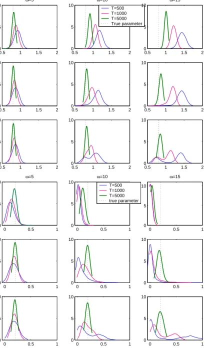
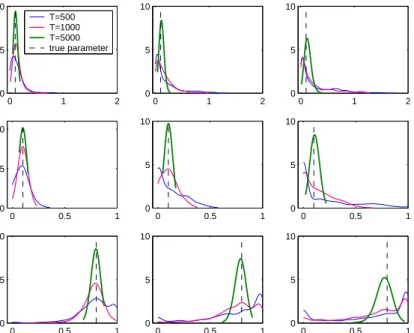
Figure 7 contains the kernel estimates of the density of αbM L
0 , αbM L1 and
b
βM L based on 1000 replicates, for a GARCH(1,1) model with parameters
α0 = 0.1, α1 = 0.1 and β = 0.8, contaminated a single outlier of sizes ω =
5,10 and 15 standard deviations. As we can see in the plots, for large sample sizes, like T = 5000, ML estimators seem to be robust to the presence of outliers. Notice that they are unbiased even when the series is contaminated by an outlier of size 15 standard deviations. This is not true for smaller sample sizes, like T = 500 or 1000, where just one outlier seems to bias towards zero the estimated αb1 and towards one the estimated value βb, in
the sense that the estimated density is bigger for those values. When we look at the results in Figure 8, containing kernel estimates of the density of αbM L
0 , αbM L1 and βbM L based on 1000 replicates, for the same GARCH(1,1)
model but now contaminated with two consecutive outliers of sizes ω= 5,10 and 15 standard deviations, it seems that αbM L
0 and αbM L1 are overestimating
the true parameters, and βb is underestimating the true β. Hence, the bias caused by outliers on the ML estimates of a GARCH(1,1) model depend also on the size of the outlier, and very important, on their position in the series.
The bias caused by isolated outliers are very different from the bias caused by consecutive ones. This could be one reason for the contradictory results found in the literature.
From the ARCH(∞) representation of a GARCH(1,1) model, we could find an explanation to the bias caused by a single outlier. Let us consider a series yt generated by a GARCH(1,1) model where σ02 = 1−αα10−β, i.e., the
initial value for σ2
t is the unconditional variance. For a sample size, T, fixed, the series can be approximated by the following ARCH(T −1) model:
( yt =εtσt σ2 t = ˜ω+ PT−1 i=1 α˜iyt2−i where ˜α0 =α0 h 1+βT−1 1−β + βT−1 1−α1−β i y ˜αi =α1βi−1 for i= 1,2, . . . , T −1.
If the observed series is contaminated with a single outlier of size ω, we have seen before that limω→∞α˜0 = ∞ y limω→∞α˜i = α1βi−1 = 1/(T −
2), ∀i. In particular, for i = 1 we would have that αb1 tends to 1/(T −2)
and therefore,βbtends to one as the size of the outlier tends to infinity. In the limit,αb1 is close to zero andβbis close to one, implying that the unconditional
variance tends to infinity and α0 would not be identified. This could explain
why ωb is not very affected by the outlier.
6
Empirical application
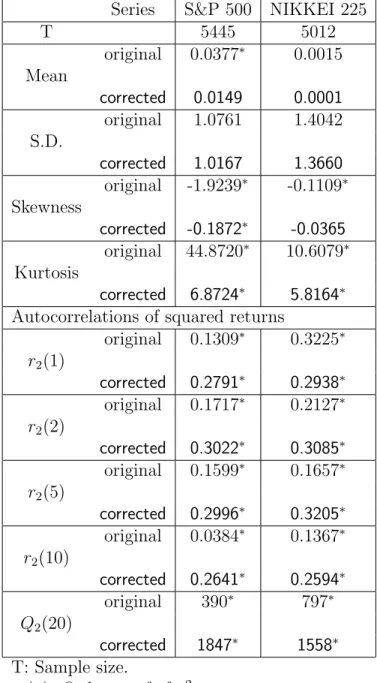
This section illustrates the previous results by analyzing two world indexes. We consider the daily series of returns of the S&P 500 index of US and the Nikkei 225 index of Japan, observed from October 20, 1982 to May 17, 2004 and from January 4, 1984 to May 19, 2004 respectively3. Figures 9 and 10
plot the return series and the correlogram of the squared observations for the original series and for the series corrected for outliers. Series have been corrected by substituting the corresponding outliers by the unconditional mean. In the S&P 500 series there is one observation which is exactly 22 times the standard deviation. This observation corresponds to the 19th of October, 1987, also known as “October black monday”, the biggest fall in all the history of Wall Street. The other two outliers correspond to the following days, October, 21 and 26. The size of these two observations is around 8.5 standard deviations. In the Nikkei 225, there are two consecutive outliers corresponding to the same “October black monday”, 19th and 20th of Octo-ber, 1987. In this case, the corresponding return was 11 times the standard deviation. The third outlier in this series corresponds to 2nd October 1990, and this observation is 8 times the standard deviation.
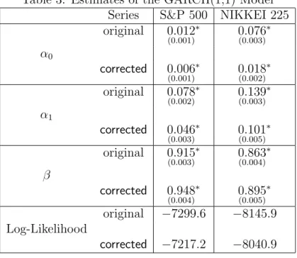
As we can observe in both figures, correcting the series by these extreme observations makes more clear the structure in the squared observations. In the case of the S&P 500, we can see how just one observation biases towards zero all correlation coefficients of squared observations, and in the Nikkei 225, two consecutive outliers overestimate the first order autocorrelation and underestimate all the others, as expected looking at the theoretical results. Table 1 contains descriptive statistics for both original and corrected series. Tables 2 and 3 contain estimated parameters for and ARCH(9) and GARCH(1,1) model. As these examples illustrate, real time series can be affected by outliers which can bias the correlogram of squared observations and affecting in a decisive way the identification and estimation of conditional heteroscedasticity. Nevertheless, for these two particular series, outliers do
not change the conclusions of the conditional homoscedasticity tests analyzed in this paper, which reject the null hypothesis of conditional homoscedastic-ity for all the series, the original and the corrected ones. However, as Tables 2 and 3 show, estimated parameters are quite different in original and corrected series.
7
Conclusions
In the presence of isolated outliers, the sizes of the LM, Q(k) and D(k) tests for conditional homoscedasticty is always zero while their powers are also zero if the sample size is relatively small while it is recovered for large enough sample sizes. The effect of consecutive outliers is even worse because, in this case, these tests always reject the hosomoscedasticity hypothesis even if the series is truly homoscedastic and the sample size is large. On the other hand, the size and power of the test proposed by... are robust to the presence of both isolated and consecutive outliers. However, the size gets larger as the sample size increases and, consequently, this test can be misleading rejecting homoscedasticity too often.
References
[1] Aggarwal, R., C. Inclan and R. Leal (1999), Volatility in Emerging Stock Markets, Journal of Financial and Quantitative Analysis, 34, 33-35. [2] Blake, N.S. and T.B. Fomby (1994), Large Shocks, Small Shocks and
Economic Fluctuations: Outliers in Macroeconomic Time Series, Jour-nal of Applied Econometrics, 9, 181-200.
[3] Bollerslev, T. (1986), Generalized Autoregressive Conditional Het-eroskedasticity, Journal of Econometrics, 31, 307-327.
[4] Bollerslev, T. (1987), A Conditionally Heteroskedastic Time Series Model for Speculative Prices and Rates of Return, The Review of Eco-nomics and Statistics, 69, 542-547.
[5] Bollerslev, T. and J.M. Wooldridge (1992), Quasi-Maximum Likelihood Estimation and Inference in Dynamic Models with Time-Varying Co-variances, Econometric Reviews, 11, 143-172.
[6] Bollerslev, T., R.F. Engle and D.B. Nelson (1994), ARCH Models, The Handbook of Econometrics, 4, 2959-3038.
[7] Chen, C. and J. Liu (1993), Joint Estimation of Model Parameters and Outlier Effects in Time Series, Journal of the American Statistical As-sociation, 88, 284-296.
[8] Doornik, J.A. and M. Ooms (2002), Outlier detection in GARCH mod-els, manuscript.
[9] Engle, R.F. (1982), Autoregressive Conditional Heteroskedasticity with Estimates of the Variance of United Kingdom Inflation, Econometrica,
50, 987-1007.
[10] Franses, P.H. and E. Ghijsels (1999), Additive Outliers, GARCH and Forecasting Volatility, International Journal of Forecasting, 15, 1-9. [11] Franses, P.H. and D. van Dijk (1999), Outlier detection in GARCH
[12] Franses, P.H., D. van Dijk and A. Lucas (2004), Short Patches of Out-liers, Applied Financial Economics, forthcoming.
[13] Geweke, J. (1986), Comment to ”Modeling persitence of conditional variance, Econometric Reviews, 5, 57-61.
[14] Gregory, A.W. and J.J. Reeves (2001), Estimation and Inference in ARCH Models in the Presence of Outliers, Proceedings of the 2002 North American Summer Meetings of the Econometric Society.
[15] Hotta, L.K. and R.S. Tsay (1998), Outliers in GARCH processes, manuscript.
[16] Lee, J.H.H. (1991), A Lagrange Multiplier Test for GARCH Models,
Economics Letters, 37, 265-271.
[17] Lee, S. and B.E. Hansen (1994), Asymptotic Theory for the GARCH(1,1) Quasi-Maximum Likelihood Estimator,Econometric The-ory, 10, 29-52.
[18] Li, J. and C. Kao (2002), A Bounded Influence Estimation and Outlier Detection for ARCG/GARCH Models with an Application to Foreign Exchange Rates, manuscript.
[19] Lumsdaine, R.L. and S. Ng (1999), Testing for ARCH in the Presence of a Possibly Misspecified Conditional Mean, Journal of Econometrics,
[20] Lumsdaine, R.L. (1996), Consistency and Asymptotic Normality of the Quasi-Maximum Likelihood Estimator in IGARCH(1,1) and Covariance Stationary GARCH(1,1) Models, Econometrica, 64, 575-596.
[21] Mendes, B.V.M. (2000), Assessing the Bias of Maximum Likelihood Es-timates of Contaminated GARCH Models, Journal of Statistical Com-putation and Simulation, 67, 359-376.
[22] McLeod, A.J. and W.K. Li (1983), Diagnostic Checking ARMA Time Series Models Using Squared-Residual Correlations, Journal of Time Series Analysis, 4, 269-273.
[23] Muller, N. and V.J. Yohai (2002), Robust Estimates for ARCH Pro-cesses, Journal of Time Series Analysis, 23, 341-375.
[24] Ng, H.G. and M.McAller (2003), Recursive modelling of symmetric and asymmetric volatility in the presence of extreme observations, Interna-tional Journal of Forecasting, forthcoming.
[25] Pantula, S.G. (1986), Comment to ”Modeling persitence of conditional variance”, Econometric Reviews, 5, 57-61.
[26] Pe˜na, D. (2001), Outliers, influential observations and missing Data, in Pe˜na, D., G.C. Tiao and R.S. Tsay (eds.), A course in Time Series, John Wiley, New York.
[27] Sakata, S. and H. White (1998), High Break-down Point Conditional Dispersion Estimation with Application to S&P500 Daily Returns Volatility, Econometrica, 66, 529-567.
[28] Taylor, S.J. (1986), Modelling Financial Time Series, John Wiley. [29] Ter¨asvirta, T. (1996), Two Stylized Facts and the GARCH(1,1) Model,
W.P. Series in Finance and Economics, 96, Stockholm School of Eco-nomics.
[30] Tsay, R.S. (1988), Outliers, Level Shifts and Variance Changes in Time Series, Journal of Forecasting, 7, 1-20.
[31] Van Dijk, D., P.H. Franses and A. Lucas (1999), Testing for ARCH in the Presence of Additive Outliers, Journal of Applied Econometrics, 14, 539-562.
[32] Verhoeven, P. and M. McAleer (2000), Modelling outliers and extreme observations for ARMA-GARCH processes, manuscript.
Figure 1: Biases caused by outliers on the correlogram of squared observa-tions 0 10 20 30 −0.1 0 0.1 0.2 0.3 0.4 0.5
Two consecutive outliers of size ω=15
0 10 20 30 −0.1 0 0.1 0.2 0.3 0.4 0.5
One single outlier of size ω=15
N(0,1), T=1000 0 10 20 30 −0.1 0 0.1 0.2 0.3 0.4 0.5 Lag 0 10 20 30 −0.1 0 0.1 0.2 0.3 0.4 0.5 Lag GARCH(1,1), T=1000
True ACF True ACF
Figure 2: Effects caused by outliers on the size and power of conditional homoscedasticity tests 0 5 10 15 20 0 0.2 0.4 0.6 0.8 1
Size of tests with one single outlier
N(0,1) nominal size Robust T=5000 Robust T=1000 Robust T=500 McLL T=5000 McLL T=1000 McLL T=500 0 5 10 15 20 0 0.2 0.4 0.6 0.8 1
Size of tests with two consecutive outliers
0 5 10 15 20 0 0.2 0.4 0.6 0.8 1
Power of tests with one single outlier
Size of the outlier
GARCH(1,1) 0 5 10 15 20 0 0.2 0.4 0.6 0.8 1
Power of tests with two consecutive outliers
Figure 3: Kernel estimation of the density of estimators of an ARCH(1) model with a single outlier
0.5 1 1.5 2 0 5 10 ω=5 α0 OLS 0.5 1 1.5 2 0 5 10 ω=10 T=500 T=1000 T=5000 True parameter 0.5 1 1.5 2 0 5 10 ω=15 0.5 1 1.5 2 0 5 10 α0 GLS 0.5 1 1.5 2 0 5 10 0.5 1 1.5 2 0 5 10 0.5 1 1.5 2 0 5 10 α0 MLE 0.5 1 1.5 2 0 5 10 0.5 1 1.5 2 0 5 10 0 0.5 1 0 5 10 ω=5 α1 OLS 0 0.5 1 0 5 10 ω=10 T=500 T=1000 T=5000 true parameter 0 0.5 1 0 5 10 ω=15 0 0.5 1 0 5 10 α1 GLS 0 0.5 1 0 5 10 0 0.5 1 0 5 10 0 0.5 1 0 5 10 α1 MLE 0 0.5 1 0 5 10 0 0.5 1 0 5 10
Figure 4: Ratio of variances of estimators of an ARCH(1) model with a single outlier 0 10 20 0 0.5 1 1.5 2 T=500 α0 OLS 0 10 20 0 5 10 15 20 25 α0 MLE 0 10 20 0 5 10 15 20 25 0 10 20 0 5 10 15 20 25 0 10 20 0 0.5 1 1.5 2 T=1000 0 10 20 0 5 10 15 20 25 α0 GLS 0 10 20 0 5 10 15 20 25 0 10 20 0 5 10 15 20 25 0 10 20 0 0.5 1 1.5 2 T=5000 ARCH White 0 10 20 0 0.5 1 1.5 2 T=500 α1 OLS 0 10 20 0 0.5 1 1.5 2 T=1000 0 10 20 0 0.5 1 1.5 2 T=5000 ARCH White 0 10 20 0 5 10 15 20 25 α1 GLS 0 10 20 0 5 10 15 20 25 0 10 20 0 5 10 15 20 25 0 10 20 0 5 10 15 20 25 α1 MLE 0 10 20 0 5 10 15 20 25 0 10 20 0 5 10 15 20 25
Figure 5: Kernel estimation of the density of estimators of an ARCH(1) model with two consecutive outliers
0.5 1 1.5 2 0 5 10 ω=5 α0 OLS 0.5 1 1.5 2 0 5 10 ω=10 T=500 T=1000 T=5000 True parameter 0.5 1 1.5 2 0 5 10 ω=15 0.5 1 1.5 2 0 5 10 α0 GLS 0.5 1 1.5 2 0 5 10 0.5 1 1.5 2 0 5 10 0.5 1 1.5 2 0 5 10 α0 MLE 0.5 1 1.5 2 0 5 10 0.5 1 1.5 2 0 5 10 0 0.5 1 0 5 10 ω=5 α1 OLS 0 0.5 1 0 5 10 ω=10 0 0.5 1 0 5 10 ω=15 0 0.5 1 0 5 10 α1 GLS 0 0.5 1 0 5 10 T=500 T=1000 T=5000 True parameter 0 0.5 1 0 5 10 0 0.5 1 0 5 10 α1 MLE 0 0.5 1 0 5 10 0 0.5 1 0 5 10
Figure 6: Ratio of variances of estimators of an ARCH(1) model with two consecutive outliers 0 10 20 0 0.5 1 1.5 2 T=500 α0 OLS 0 10 20 0 0.5 1 1.5 2 T=1000 0 10 20 0 0.5 1 1.5 2 T=5000 ARCH White 0 10 20 0 5 10 15 20 25 α0 GLS 0 10 20 0 5 10 15 20 25 0 10 20 0 5 10 15 20 25 0 10 20 0 5 10 15 20 25 α0 MLE 0 10 20 0 5 10 15 20 25 0 10 20 0 5 10 15 20 25 0 10 20 0 0.5 1 1.5 2 T=500 α1 OLS 0 10 20 0 0.5 1 1.5 2 T=1000 0 10 20 0 0.5 1 1.5 2 T=5000 ARCH White 0 10 20 0 5 10 15 20 25 α1 GLS 0 10 20 0 5 10 15 20 25 0 10 20 0 5 10 15 20 25 0 10 20 0 5 10 15 20 25 α1 MLE 0 10 20 0 5 10 15 20 25 0 10 20 0 5 10 15 20 25